Bifurcation and stability analyses of horizontal Bridgman crystal growth of a low Prandtl number material

Bifurcation and stability analyses of horizontal Bridgman

crystal growth of a low Prandtl number material

C.W. Lan*, M.K. Chen, M.C. Liang

Chemical Engineering Department, National Taiwan University, Taipei 10617, Taiwan, ROC

Received 26 September 1997; accepted 20 November 1997

Abstract

Stability and bifurcation analyses are conducted for horizontal Bridgman crystal growth of a low Prandtl number material. The model considers two-dimensional heat transfer and fluid flow in the melt, the growth interface, and the heat conduction in the crystal. In addition to the construction of bifurcation diagrams, the stability of various solution families is further examined by their leading eigenvalues based on linear stability analysis. Transient calculation is also performed to illustrate the global behavior of the basic states after a disturbance. For the cases with a fixed interface, the results for periodically oscillatory flows are in good agreement with previous reports. With a free interface, the bifurcation diagram is slightly changed due to interface deformation, but its qualitative characteristics remain the same. Nevertheless, the dynamic evolution of the interface due to convection provides useful information for crystal growth. The oscillation amplitude of the interface velocity, which decreases with the increasing heat of fusion, is in the same order of a common growth rate used in practice. ( 1998 Elsevier Science B.V. All rights reserved.

PACS: 44.25.#f; 47.27.Te; 81.10.Fq; 02.60.Cb; 02.70.Fj

Keywords: Stability; Bifurcation; Buoyancy convection; Interface; Horizontal Bridgman

1. Introduction

The horizontal Bridgman (HB) technique is one of the most important methods for the single crystal growth of compound semiconductors [1], especially GaAs. Because of the larger horizontal

* Corresponding author: Fax: #886 2 23633917; e-mail:

[email protected].

thermal gradients and aspect ratio, stronger con-vection and more complicated flow structures and transition can be induced. Especially, the transition to oscillatory flows that might be detrimental to the growth has attracted much attention of crystal growers and fluid mechanists. Since the pioneering experiments on gallium melt by Hurle et al. [2,3] illustrating interesting oscillatory flows, many theoretical studies (e.g., Refs. [4—9]) have been de-voted to the flow instability of HB growth of low Prandtl (Pr) number materials. Some benchmark

0022-0248/98/$19.00( 1998 Elsevier Science B.V. All rights reserved.

comparison using different numerical schemes have also been proposed in a special GAMM workshop [10]. Therefore, the importance of this problem is clear. Recently, Skeldon et al. [9] also presented a more detailed description of the global oscillatory convection. Two types of Hopf bifurcations were investigated. Careful temperature measurements for the gallium melt and the comparison with a 2D model have also been reported recently [11]. Un-fortunately, most of the studies so far have not included the deformed (moving) growth interface into account. In reality, the unstable convection is regarded as a major source for oscillatory growth rate and thus growth striations causing nonuni-formity in the grown crystals. Therefore, the coupled behavior of the moving interface and the flows is important in practice.

The modeling of two-dimensional (2D) HB growth with a deformed interface was studied by Crochet et al. [12] for the first time. Oscillatory flows at Ra"4750 were illustrated, but the bifurca-tion and stability analyses were not conducted. As mentioned by Winters [3], the meshes used in their calculations were too coarse to present the results accurately. The extension of their model to a three-dimensional (3D) one but without the interface was also presented [4]. In the most recent work by Liang and Lan [13], a 3D model with the consid-eration of the growth interface was proposed. The effects of buoyancy and Marangoni convections and growth conditions on the growth interface were studied. However, the bifurcation behavior and oscillatory flows as well as their effects on the growth interface were not considered. So far, a de-tailed 3D numerical computation of flow bifurca-tion and stability is still too costly to conduct. A 2D model with the growth interface, though oversim-plified, is still useful in some fundamental under-standing for the HB crystal growth.

In this paper, the bifurcation and stability ana-lyses as well as the dynamic evolution of flows and interface velocity for a 2D HB model are conduc-ted. Benchmark comparison of our calculated re-sults for the fixed-interface problems with previous reports is presented first for various boundary con-ditions. Bifurcation diagrams are further construc-ted using a finite-volume/Newton method with the pseudo-arclength continuation. The stability of the

solution is also examined by leading eigenvalues based on linear stability analysis. Furthermore, the dynamic responses of the basic stationary solutions from the bifurcation diagrams by a small dis-turbance are investigated through transient calcu-lations; the effect of heat of fusion is then con-sidered. The model description is presented in the next section, followed by the numerical methods in Section 3. Section 4 is devoted for results and dis-cussion. In Section 5, short conclusions are drawn.

2. Model description

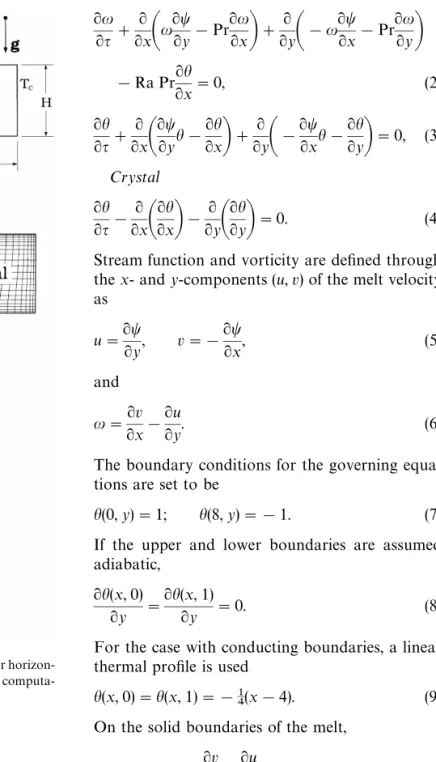
The schematic of a 2D HB growth model is shown in Fig. 1a. In order to have the same back-ground for comparison with previous reports, the crucible is neglected. The height of the melt is

H and the length 2¸. The aspect ratio A(¸/H) for

the melt, for the fixed interface, is chosen to be 4 for comparison purposes. However, since the interface shape and position are affected by convection, the actual aspect ratio slightly differs from 4. The inter-face shape h(y) is unknown a priori and needs to be solved simultaneously with field variables. The temperature on both ends is fixed at ¹H and ¹C, respectively, while ¹. (the melting point) is fixed at the growth interface. Either the adiabatic or the conducting boundary condition is used for the up-per and lower boundaries. All the melt boundaries are solid, except the upper one, which can be stress-free. Physical properties of the material are assumed constant, while the melt is incompressible. Thermal properties of the solid and melt phases are assumed to be the same. Again, such assumptions are only for the convenience of comparison.

Dimensionless variables are defined by scaling the length with H, velocity with a./H, and time with H2/a., where a. is the thermal diffusivity. The dimensionless temperature (h) is defined as h,(¹!¹m)/(¹H!¹m). For the convenience of illustration, ¹C is adjusted so that h is equal to !1 at the right boundary. The coordinates x and y, the interface h, velocity components u and v, and the time q used afterwards are all dimensionless. The Boussinesq approximation [14] is also adopted in the flow calculation. The conservation equations in a dimensionless form for the 2D incompressible

Fig. 1. (a) Schematic sketch of the simplified model for horizon-tal Bridgman cryshorizon-tal growth; (b) a sample mesh for computa-tion; (c) a typical control volume.

laminar flow of a Newtonian fluid and heat transfer in the melt, as well as heat conduction in the crystal, can be described in terms of stream function t, vorticityu, and temperature h as follows:

Melt ­2t ­x2# ­2t ­y2#u"0, (1) ­u ­q# ­ ­x

A

B

A

B

­q#­x­

A

B

A

B

Crystal ­h ­q! ­ ­x

A

B

A

B

The boundary conditions for the governing equa-tions are set to be

h(0, y)"1; h(8, y)"!1. (7) If the upper and lower boundaries are assumed adiabatic,

­h(x, 0) ­y "

­h(x, 1)

­y "0. (8) For the case with conducting boundaries, a linear thermal profile is used

h(x, 0)"h(x, 1)"!14(x!4). (9) On the solid boundaries of the melt,

t"0, u"­v ­x! ­u ­y, (10) subject to u"v"0. (11)

For the case with a shear-free upper boundary condition, t"u"0 at the free surface. Maran-goni convection can be considered as well, but it will not be discussed in this report.

At the melt/solid interface, the interface energy balance is imposed as !St­h ­q# ­h ­n

K

K

h"0. (13)

In Eq. (12), St,*H/Cp.(¹H!¹C) is the Stefan number; *H is the heat of fusion and Cp. the specific heat of the melt.i is the ratio of the thermal conductivity of the solid to the melt, and it is set to be one here for comparison purposes. The Prandtl (Pr) and Rayleigh (Ra) numbers used in the govern-ing equations are defined as:

Pr,l./a., Ra,gb(¹H!¹.)H3/(l.a.), wherel. is the kinematic viscosity, b the thermal expansion coefficient, and g the gravitational accel-eration.

3. Numerical solutions

Due to the unknown and deformed interface shape h(y), a finite volume method (FVM) [15] based on the body-fitted coordinates is adopted. Fig. 1b shows a sample mesh; the mesh lines define the boundaries of finite or control volumes (CVs). A typical CV in the physical space is illustrated in Fig. 1c, where g and m are the coordinates in the computational domain. The idea of FVM is simply to integrate the governing equations over every CV. For example, for each CV, after the Gauss theorem is applied, a flux balance equation for the variables can be obtained with the following form:

Ie!Iw#In!Is#

P

P

( is the source term of the governing equations and *V the volume of CV. Each of the fluxes Ii is made of two distinct parts, namely a convective contribu-tion and a diffusive contribucontribu-tion; the mesh

move-ment also needs to be considered in the convective part. Both terms are approximated with the central difference scheme. Upwinding is found unnecessary here. Detailed implementation of the scheme can be found elsewhere [15,16]. For stationary solutions, the time-dependent terms are removed.

In order to locate multiple steady states for sta-tionary solutions and to avoid the singular Jac-obian matrix at bifurcation or limiting (turning) points, the pseudo-arclength continuation tech-nique [17] is further adopted. The idea of continua-tion is to trace the solucontinua-tion along a branch family through an arclength s by including an additional equation for the continuation parameter. For example, if Ra is chosen as the continuation par-ameter, the additional equation can be written as the following ­xT ­s

K

K

By appending the continuation equation to the steady-state flux balance equations (Eq. (14) with-out the time-dependent terms) for all CVs in the domain, as well as the isotherm condition (Eq. (13)), a set of nonlinear algebraic equations can be obtained

f (y),0, (16)

where y"[x, Ra]T. Eq. (16) is solved by Newton’s method for all variables simultaneously. During Newton’s iteration, the Jacobian matrix JI , defined as­fi/­yj, is estimated by the forward difference and the Newton’s linear equations are solved by the ILU(0) preconditioned GMRES method [18]. In fact, since J_{I is very sparse, its construction only} needs a small number of residual evaluations, and the computational effort is only about 20% of that for solving linear equations. Furthermore, the use of the iterative matrix solver greatly reduces the memory required and is thus suitable for larger problems.

For transient solutions, a set of differential/alge-braic equations (DAEs) can be obtained from Eq. (14) as

M(x)dx

dq"f (x; Ra), (17) where M(x) is the mass matrix and it is singular because some equations, e.g., the stream equations, do not have an explicit time dependent term. If a basic state x0 is found by Newton’s method dur-ing continuation, for the basic state x0, linear stabil-ity analysis can be implemented by substituting

x"x0#eepq into the above equation, where e is

a small disturbance vector. After the linear terms of

e are collected, a generalized eigenvalue problem is

obtained

pM(x0)e"JI(x0)e. (18) Apparently, the Jacobian JI obtained after New-ton’s iterations can be used here directly. The stability of the basic state x0 can also be easily determined by the sign of the eigenvaluep. In other words, in Eq. (18) if there is any positive eigenvalue, the basic state x0 is not stable to an infinitesimal disturbance. Hopf bifurcation can also be detected by the appearance of a pair of pure imaginary conjugated eigenvalues. It should be pointed out that linear stability is not applicable to a finite disturbance. With a finite disturbance, a stable solution based on linear stability may not be always stable. To examine the linear stability, only the lar-gest eigenvalue needs to be computed, and this re-duces the effort of stability analysis significantly. ARPACK [19] is then used to calculate the leading eigenvalues, while the matrix inversion is performed by the ILU(0) preconditioned GMRES method.

The fully transient solution of Eq. (14) is solved by DASPK [20], a Krylov-subspace [21] based DAE solver. The preconditioner for the solution of nonlinear equations at each time step during integ-ration is, again, the ILU(0) of the numerical Jac-obian matrix. Although DASPK is quite robust, the choice of the preconditioners is important to its convergence at each time step. A consistent initial condition is important as well. The basic state cal-culated by Newton’s method described previously is used as the initial condition here.

4. Results and discussion

In this section, we will start from some bench-mark comparison with previous results for the cases with a fixed interface first. Since the unusual flow structures at medium Ra numbers are the most interesting part [9—11] and the dynamic phe-nomena are very rich, we will focus our discussion only to medium Ra numbers. Furthermore, from the comparison of the thermal profile from 2D calculations with experiments [11], in this convec-tion regime the effect of the lateral walls is small, which makes the 2D approximation reasonable. After the benchmark comparison for the fixed-in-terface cases, the effects of the free infixed-in-terface will then be illustrated through the bifurcation diagram and dynamic responses to a small disturbance. The reliability of the eigenvalues from the numerical Jacobian and effects of heat of fusion will also be discussed.

4.1. Benchmark comparison for fixed-interface problems

Since some results for the cases with a fixed interface are available (e.g., Ref. [5]), benchmark comparison and mesh refinements are illustrated first. For the case of Pr"0.015 with rigid and insulating upper and lower boundaries, the bifurca-tion diagram is shown in Fig. 2. Some flow struc-tures are also included to illustrate different flow families and multiple steady states. When the Ra number is small, the flow structure is one-cell, e.g., the solution a. The distortion of the one-cell flow increases with increasing Ra number, and finally becomes corotational three-cell like the solution c. A Hopf bifurcation is found at Ra+2164, where the complex pair of the leading eigenvalues has a zero real part;p"$1.954i. The corresponding frequency (dimensionless) is 1.954/2p. After the Hopf point, the solution is not stable and is repre-sented by a dashed line.

Another branch beneath the primary solution is found as well, and the flow structure is mainly a corotating two-cell. It should be pointed out that the unstable corotating two-cell solution in the bifurcation diagram usually is difficult to obtain. With the continuation technique, the turning point

Fig. 2. Bifurcation diagram for the fixed-interface problem with rigid and insulating upper and lower boundaries; Pr"0.015 and A"4; the dashed-line indicates the unstable solution branch.

Table 1

Comparison of Hopf points and frequencies with the ones by Winters [5]

B.C. (upper) Grid _Ra# Frequency

Insulating, 90]36 2164 0.311 rigid 121]49 2062 0.307 (Winters) 121]49 2285 0.317 Conducting, 90]36 1823 0.280 rigid 121]49 1745 0.271 (Winters) 121]49 1690 0.262 Insulating, 90]36 1034 0.206 stress free 121]49 1008 0.204 (Winters) 121]49 996 0.203 Conducting, 90]36 908 0.194 stress free 121]49 892 0.194 (Winters) 121]49 886 0.192

and the stationary solution after Hopf bifurcation can still be obtained easily. The starting point of the lowest branch for the continuation can be obtained easily from the solution at a higher Ra, e.g., Ra"4000. In general, with a fully transient calcu-lation, the unstable branch cannot be found. In-stead, the hysteresis between the upper and lower stable solution branches is a typical observation [6—8]. The bifurcation diagrams for Pr"0—0.015 and different boundary conditions are all similar to Fig. 2. However, for the shear-free and insulating upper boundary, the lower branch is not found. Furthermore, the dynamic phenomena after the Hopf bifurcation are sensitive to parameters [9].

The comparison of the onset of oscillatory flow (the critical Rayleigh number, Ra#, or the Hopf bifurcation point) with those by Winters [5] for various boundary conditions and meshes is sum-marized in Table 1. As shown, based on a similar mesh (the same amount of nodal points and a uni-form mesh), a reasonably good agreement with Winters’ results is obtained. The critical oscillation frequencies, f#, are calculated from the imaginary part of the leading eigenvalues, and they are

dimen-sionless. The mesh is also an important factor to the accuracy of the results. Due to the large aspect ratio, finer grid spacing in the x-direction is neces-sary. The effect of mesh on flow patterns is less sensitive. Some results for mesh refinement are il-lustrated in Fig. 3 for comparison. As shown, the flow patterns are affected very little by the mesh if the mesh is fine enough. Further comparison with a different numerical approach based on the primi-tive variables (the so-called UVP formulation) [16] is performed. The comparison is summarized in Table 2; the Nusselt number (Nu) in Table 2 is defined as the averaged heat flux over the interface. As shown, excellent agreement for both flow inten-sity and leading eigenvalues is obtained. The com-parison for problems with a free interface can be found elsewhere [16].

4.2. Bifurcation diagram for problems with a free interface

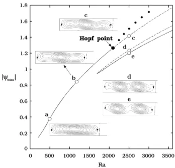
When the interface is considered for the insulated and rigid upper and lower boundaries, the interface shape and position are modulated by the flow. The bifurcation diagram is illustrated in Fig. 4; again, Pr"0.015. As shown, the solution structure is sim-ilar to that with the fixed interface, but the curves are slightly shifted downward. When the flow is

Fig. 3. Effect of meshes on the flow patterns; Ra"2500 and rigid and insulating upper and lower boundaries.

Table 2

Comparison of some calculated values from stream func-tion/vorticity (t/u) and primitive variable (UVP) approaches for Ra"2285 Mesh Nu t.*/ p t/u 0.293 !1.374 0.024$2.078i 90]36 UVP 0.290 !1.314 0.027$2.016i t/u 0.292 !_{1.362 0.070$2.018i} 120]48 UVP 0.290 !_{1.304 0.066$2.017i}

weak, e.g., at Ra"500, the flow is rather simple and is one-cell. The interface shape is not affected much. As Ra increases, the flow cell starts to distort, e.g., at Ra"1200. Again, it is a corotating three-cell flow. The interface deformation also increases. The Hopf bifurcation occurs at Ra+2046, which is slightly smaller than that with a fixed interface

(Ra"2164). The frequency is reduced from 0.317 to 0.270. The stationary solution after the Hopf point, indicated by the dash-line, is also not stable. As compared with Fig. 2, the turning point at the lower branch occurs significantly earlier as well. Furthermore, the flow intensity at the same Ra number is slightly smaller due to the more relaxed domain caused by interface deformation. The max-imum oscillatory flow intensity, calculated from transient results, is indicated by black circles. The amplitude *t (*t"t.!9!t.*/), grows from zero, and increases proportional to (Ra ! Ra#)0.5, which is a common scaling for a supercritical Hopf bifurcation. Further discussion on the transient re-sults will be presented shortly.

The effects of the free interface on the Hopf bifurcation for other boundary conditions are sum-marized in Table 3 (based on the mesh of 90]36). As shown, with the conducting boundary condi-tion, since the interface positions at the top and the bottom are fixed, the effect of the free interface on

Fig. 4. Bifurcation diagram for the free-interface problem with rigid and insulating upper and lower boundaries; the dashed-line indicates the unstable branch. The black dots after the Hopf bifurcation are taken from oscillatory solutions obtained from transient calculations.

Table 3

Effect of the interface on Hopf points and frequencies B.C. (upper) Grids _Ra# Frequency Insulating, rigid (Fixed) 90]36 2164 0.311 (Free) 90]36 2046 0.270 Conducting, rigid (Fixed) 90]36 1823 0.280 (Free) 90]36 1801 0.277 Insulating, stress free (Fixed) 90]36 1034 0.206 (Free) 90]36 1378 0.227 Conducting, stress free (Fixed) 90]36 908 0.194 (Free) 90]36 912 0.195

the Hopf bifurcation is small. With a rigid upper boundary, the inclusion of the free-interface de-creases both Ra# and f#. However, for the stress-free upper boundary, the effect is the opposite; both Ra# and f# increase. In summary, the deformation of the interface increases the melt aspect ratio, and thus affects the Hopf point and the oscillation frequency as well as the turning point.

4.3. Transient responses

The bifurcation and linear stability analyses pre-sented previously are efficient, but they only predict a local behavior of a stationary solution. For a glo-bal behavior and dynamic phenomena, a fully tran-sient calculation is necessary; however, it is much more time consuming. With previous analyses, we are ready to examine the global behavior of the stationary solution. Three steady-state solutions at Ra"2500 (solutions c, d, and e in Fig. 4) are chosen for study. Again, among these three solu-tions, only the solution e is stable. To study the dynamic behavior of the solutions, a very small disturbance is applied to the stationary states. For

the solution c, the dynamic evolution of the max-imum stream functiont.!9 and the interface velo-city at y"0.5, as well as some typical flow patterns are shown in Fig. 5. Fig. 5a shows the dynamic responses of the maximum flow intensity. As shown, periodically oscillatory flows are developed after the disturbance, and finally a harmonic oscil-lation with a constant amplitude is obtained. As a result of the oscillatory flow, the interface velo-city, e.g., dh/dq, at y"0.5 is also oscillatory, as shown in Fig. 5b. In such a case, it is believed that the oscillatory interface velocity, i.e., the growth and melting rate, can cause the growth striations. Taking a 1-cm depth InP melt as an example, the oscillation amplitude of the interface velocity is about 5.56 cm/h, which is much larger than a com-mon growth rate (several mm/h) used in practice. However, in this case, the heat of fusion has not been considered, which will be discussed shortly in Section 4.4. In addition, as expected, the oscillation frequency from Fig. 5 ( f#"0.294) is consistent with that from eigenvalues ( f#"0.301).

The evolution of the flow patterns of one period nearq"45 are illustrated in Fig. 5c. As shown, the flow structures change periodically, and the change

Q

Fig. 5. Dynamic response of the solution at Ra"2500 (from solution c in Fig. 4) after a small disturbance: (a) maximum flow intensity; (b) interface velocity; (c) a cycle of flow patterns.

is quite significant. Such a three-cell/one-cell oscil-lation is similar to that reported by Winters [5]. The dynamic responses of solutions d and e are less interesting. After a short transient period, only the solution e is the final state.

The numerical Jacobian used in this study has allowed us to tackle a complicated problem with-out paying much attention to its details (analytical derivation). However, the reliability of the leading eigenvalues based on the numerical Jacobian is an open question, and a careful examination is neces-sary. In order to check that, in addition to Ra"2500, we have compared the frequencies ob-tained from the imaginary part of leading eigen-values for other Ra numbers with the ones obtained directly from the transient calculations. A good agreement is found for Ra"1500, 2010, and 2500; at Ra"1500,p"!0.156$1.45i, and thus f#" 0.231 (0.229 from transient calculation), at Ra" 2010,p"!0.003$1.7i, f#"0.271 (0.267), and at Ra"2500,p"0.242$1.89i, f#"0.301 (0.294). In fact, we have also used the central difference scheme, which requires double CPU effort, to evaluate the Jacobian matrix, but the difference is trivial. Therefore, numerical Jacobian is believed reliable in this study. Its applications on other problems, e.g., the Rayleigh—Benard problem [22], are found satisfactory as well.

The dynamic response at Ra"3000 is examined further. As shown in Fig. 6, the solution starts to oscillate after the disturbance is applied. However, the three-cell solution a, after a few oscillation cycles, quickly tends to the stable two-cell solution b, which is located at the lowest branch of Fig. 4. In other words, the upper branch after Ra"3000 is for sure not a ‘stable’ periodic flow. In fact, it is hard to examine the stability of the solution between the Hopf point and Ra"3000. For the flow that is not far away from the Hopf point, the oscillation can sustain for quite some time without showing any sign of decay. Furthermore, as mentioned pre-viously, the amplitude of the flow oscillation (t.!9!t.*/) grows and is proportional to

Fig. 7. Effect of heat of fusion on the interface velocity for Ra"2500. Fig. 6. Dynamic response of the flow intensity at Ra"3000

after a small disturbance; the solution a is located at the upper branch (after the Hopf bifurcation) in Fig.4, while the solution b is located at the lower one.

(Ra!Ra#)0.5. Although this behavior looks like a supercritical Hopf bifurcation, the runaway solu-tion at Ra"3000 also implies that somewhere before this point there is a loss of Hopf stability.

This observation may be explained by the Hopf/Hopf unfolding proposed by Skeldon et al. [9], where a stable quasiperiodic solution also exists between the first and the second Hopf bifurcations. In fact, we also find quasiperiodic flows from a long-term response, which will be illustrated shortly.

4.4. Effects of heat of fusion

In all of the previous calculations, the Stefan number St is set to zero for comparison purposes. In other words, the effect of heat of fusion is ne-glected. Since the system is stationary (without cru-cible movement), the bifurcation diagram is not affected by St numbers at all for steady-state solu-tions. However, if the solution is oscillatory (after the Hopf point), the heat of fusion may be impor-tant. For example, if we repeat the calculation with nonzero St for Ra"2500, as illustrated in Fig. 7, the effects are not trivial. As shown, the oscillatory amplitude is greatly reduced with the increasing St number. Interestingly, the frequency remains al-most the same for different St numbers. The Hopf point is also affected slightly; Ra# increases slightly as St increases. It is believed that the heat of fusion increases the inertia of the system. As the growth

rate is positive (growth), heat is released by the interface, while heat is absorbed for melting provid-ing a resistance for interface movement. If we observe Eq. (12), St is the coefficient of dh/dq. In-creasing St will reduce dh/dq for the same amount of heat flux difference generated by the oscillatory convection. Again, at St"10, which is roughly a typical value for most of the compound semiconduc-tors, the amplitude of oscillation ($0.0015) is still in the same order of the crystal growth rate used in practice; the amplitude is about 0.46 cm/h for InP melt with H"1 cm for ¹H!¹C"50°C. In other words, the growth and remelting due to the oscilla-tion of the flow is very likely. In fact, even without remelting, the oscillatory growth rate can generate striations as well. Further increasing Ra, the ampli-tude of dh/dq will grow (J(Ra!Ra#)0.5), and its effect on crystal growth will be even more significant. Another interesting observation from the dy-namic responses is their long-term behavior. As shown in Fig. 7, the periodic solutions become quasiperiodic for q'70. The quasiperiodic flows were also reported before [10,11] for Pr"0 with the fixed interface, and their connection to the second Hopf bifurcation was proposed by Skeldon et al. [9].

5. Conclusions

The bifurcation, stability, and oscillatory convec-tion of the HB growth of a low Pr material are illustrated using a 2D model with the consideration of the growth interface. The calculated results for fixed-interface cases are in good agreement with previous ones. With a free interface, the bifurcation diagram is slightly shifted, but the solution struc-ture remains the same qualitatively. Due to the convection, the melt aspect ratio is increased slight-ly. For the rigid upper boundary, the Hopf and turning points occur earlier, and the oscillation frequency is reduced. For the stress-free upper boundary, the Hopf point moves backwards and the frequency increases. The interface oscillation is induced by the unstable flow, and the interface velocity is significantly larger than a common growth rate used in practice for zero heat of fusion. The oscillation amplitude decreases with the in-creasing heat of fusion, but it is still larger, or at

least of the same order of magnitude, than a com-mon crystal growth rate. Finally, quasiperiodic flows after Hopf bifurcation are found from long-term dynamics.

Acknowledgements

This work is supported by the National Science Council of the Republic of China under Grant No. NSC 87-2214-E-008-008. CWL also thanks Prof. Sorensen of Rice University for making ARPACK available.

References

[1] E. Monberg, in: D.T.J. Hurle (Ed.), Handbook of Crystal Growth 2a: Basic Techniques, North-Holland, Amster-dam, 1994, p. 52.

[2] D.T.J. Hurle, Phil. Mag. 13 (1966) 305.

[3] D.T.J. Hurle, E. Jakeman, C.P. Johnson, J. Fluid Mech. 64 (1974) 565.

[4] M.J. Crochet, F.T. Geyling, J.J. Van Schaftingen, Int. J. Numer. Meth. Fluids 7 (1987) 29.

[5] K.H. Winters, Int. J. Numer. Meth. Eng. 25 (1988) 401. [6] B. Roux, H.B. Hadid, J. Crystal Growth 97 (1989) 201. [7] H.B. Hadid, B. Roux, J. Crystal Growth 97 (1989) 217. [8] J.P. Pulicani, E.C. Del Arco, A. Randriamampianina, P.

Bontoux, R. Peyret, Int. J. Numer. Meth. Fluids 10 (1990) 481.

[9] A.C. Skeldon, D.S. Riley, K.A. Cliffe, J. Crystal Growth 162 (1996) 95.

[10] B. Roux (Ed.), Notes on Numerical Fluid Mechanics, vol. 27, 1990.

[11] M.G. Braunsfurth, A.C. Skeldon, A. Juel, T. Mullin, D. Riley, J. Fluid Mech. 342 (1997) 295.

[12] M.J. Crochet, F.T. Geyling, J.J. Van Schaftingen, Int. J. Crystal Growth 65 (1983) 166.

[13] M.C. Liang, C.W. Lan, J. Crystal Growth 180 (1997) 587. [14] L.D. Landau, E.M. Lifshitz, in: Fluid Mechanics, vol. 6, 2nd ed., Pergamon Press, Elmsford, New York, 1987, p. 217. [15] C.W. Lan, Int. J. Numer. Meth. Fluid 19 (1994) 41. [16] M.C. Liang, C.W. Lan, J. Comp. Phys. 127 (1996) 330. [17] H.B. Keller, in: P.H. Rabinowiz (Ed.), Applications of

Bifurcation Theory, Academic Press, New York, 1977, p. 359. [18] Y. Saad, M.H. Schultz, SIAM J. Sci. Stat. Comput. 7 (1986)

856.

[19] D.C. Sorensen, SIAM J. Mater. Anal. Appl. 13 (1992) 357. [20] P.N. Brown, A.C. Hindmarsh, L.R. Petzold, SIAM J. Sci.

Comput. 15 (1994) 1467.

[21] P.N. Brown, Y. Saad, SIAM J. Sci. Stat. Comput. 11 (1990) 450.

[22] C.W. Lan, M.K. Chen, M.C. Liang, Phys. Fluids, under revision.