Discovering Fuzzy Inter- and Intra-Object
Associations
Tzung-Pei Hong1,2*, Cheng-Ming Huang3 and Shi-Jinn Horng4
1Department of Computer Science and Information Engineering National University of Kaohsiung, Kaohsiung, 811, Taiwan
2Department of Computer Science and Engineering National Sun Yat-sen University, Kaohsiung, 804, Taiwan
3Department of Electrical Engineering
National Taiwan University of Science and Technology, Taipei, 106, Taiwan 4Department of Computer Science and Information Engineering National Taiwan University of Science and Technology, Taipei, 106, Taiwan
tphong@nuk.edu.tw, apcmhl@ms8.hinet.net, horng@mouse.ee.ntust.edu.tw
Abstract
Data mining is the process of extracting desirable knowledge or interesting patterns from existing databases for specific purposes. Recently, the fuzzy and the object concepts have been very popular and used in a variety of applications, especially for complex data description. This paper thus proposes a new fuzzy data-mining algorithm for extracting interesting knowledge from quantitative transactions stored as object data. Each item itself is thought of as a class, and each item purchased in a transaction is thought of as an instance. Instances with the same class (item name) may have different quantitative attribute values since they may appear in different transactions. The proposed fuzzy algorithm can be divided into two main phases. The first phase is called the fuzzy intra-object mining phase, in which the linguistic large itemsets associated with the same classes (items) but with different attributes are derived. Each linguistic large itemset found in this phase is thought of as a composite item used in phase 2. The second phase is called the fuzzy inter-object mining phase, in which the large itemsets are derived and used to represent the relationship among different kinds of objects. An example is used to illustrate the algorithm. Experimental results are also given to show the effects of the proposed algorithm.
Keywords: association rule, data mining, fuzzy set, object-oriented transaction.
--- * corresponding author
1. Introduction
Knowledge discovery in databases (KDD) has become a process of considerable interest in recent years as the amounts of data in many databases have grown tremendously large. KDD means the application of nontrivial procedures for identifying effective, coherent, potentially useful, and previously unknown patterns in large databases [13]. The KDD process generally consists of the following three phases [12, 26]: pre-processing, data mining and post-processing. Due to the importance of data mining to KDD, many researchers in database and machine learning fields are primarily interested in this new research topic because it offers opportunities to discover useful information and important relevant patterns in large databases, thus helping decision-makers easily analyze the data and make good decisions regarding the domains concerned.
Recently, the fuzzy and the object concepts have been very popular and used in different applications, especially for complex data description. Fuzzy set theory was first proposed by Zadeh and Goguen in 1965 [41]. It is primarily concerned with quantifying and reasoning using natural language in which words can have ambiguous meanings [16, 25, 40]. This can be thought of as an extension of traditional crisp sets, in which each element must either be in or not in a set. A special notation is often
used in the literature to represent fuzzy sets. Assume that x1 to xn are the elements in fuzzy set A, and 1 to n are, respectively, their grades of membership in A. A is then
usually represented as follows:
A1/x12/x2...n/xn.
The scalar cardinality of a fuzzy set A defined on a finite universal set X is the summation of the membership grades of all the elements of X in A. These concepts
will be used in the proposed algorithm to find linguistic association rules. As to the object concept, an object represents an instance with several related attribute values and methods integrated together. They have widely applied in the fields such as databases, software engineering, knowledge representation [9, 10], geographic information systems and even computer architecture [24, 37].
In the past, data-mining is most commonly used in attempts to induce association rules from transaction data. In this paper, we will try to generalize it and propose a mining algorithm to derive linguistic association rules from quantitative object data. The proposed algorithm is divided into two main phases, one for intra-object linguistic association rules, and the other for inter-object linguistic association rules. Two apriori-like [4] procedures are adopted to find the two kinds of rules.
The remaining parts of this paper are organized as follows. Related mining algorithms are reviewed in Section 2. The object-oriented concept is introduced in Section 3. The proposed fuzzy data-mining algorithm for object-oriented quantitative transaction data is described in Section 4. An example to illustrate the proposed mining algorithm is given in Section 5. Experimental results are shown in Section 6. Conclusions and proposal of future work are given in Section 7.
2. Review of related mining approaches
The goal of data mining is to discover important associations among items such that the presence of some items in a transaction will imply the presence of some other items. To achieve this purpose, Agrawal and his co-workers proposed several mining algorithms based on the concept of large itemsets to find association rules in transaction data [1-4, 33]. They divided the mining process into two phases. In the first phase, all large itemsets were found. In the second phase, association rules were induced from the large itemsets. In addition to proposing methods for mining association rules from transactions of binary values, Agrawal et al. also proposed a method [32] for mining association rules from transactions with quantitative and categorical attributes. Their proposed method determined the number of partitions for each quantitative attribute, and then found large itemsets and association rules.
Agrawal and Srikant also proposed the AprioriAll mining approach to mine sequential patterns from a set of transactions [3]. Five phases were included in this approach. In the first phase, the original transactions were converted into customer sequences. In the second phase, the set of all large itemsets were found from the customer sequences. In the third phase, each large itemset was mapped to a contiguous integer and the original customer sequences were transformed into the mapped integer sequences. In the fourth phase, the set of transformed integer sequences were used to find large sequences among them. In the fifth phase, the maximally large sequences were derived and output to users.
As to handling numerical attributes, Fukuda et al. introduced the optimized association-rule problem and used a dynamic programming algorithm to solve it. Their approach could allow association rules to contain only a single numerical attribute on the left-hand side [14]. Rastogi and Shim then extended the approach to more than one optimal region, and showed that the problem was NP-hard even for cases involving one uninstantiated numeric attribute [29]. In addition, several fuzzy learning algorithms for inducing rules from given sets of data have been designed and used to good effect with specific domains [5, 7-8, 11, 15, 17-23, 25, 30, 34-35]. Strategies based on decision trees [9] were proposed in [7, 27-28, 30-31, 36, 38], and based on the version space learning were proposed in [34].
As to fuzzy mining, Hong et al. proposed a fuzzy mining algorithm to mine fuzzy rules from quantitative data [18]. They transformed each quantitative item into a fuzzy set and used fuzzy operations to find fuzzy rules. Cai et al. proposed weighted mining to reflect different importance to different items [6]. Each item was attached a numerical weight given by users. Weighted supports and weighted confidences were then defined to determine interesting association rules. Yue et al. then extended their concepts to fuzzy item vectors [39]. Many related researches are still in progress.
In this paper, a fuzzy mining algorithm is proposed for finding inter- and intra-object association rules from quantitative object transactions. It includes two
apriori-like fuzzy procedures.
3. Object-oriented transactions
An object-oriented transaction includes one or more purchased items, each of which is represented as an object or an instance. Each instance inherits its characteristics from a superior object, called class, which defines the basic structure of objects with common properties, including attributes, default values, and methods. The roles of classes and instances in an object-oriented transaction data are like those that schema and tuples play in a relational database [37].
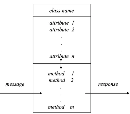
A simple structure of a class is shown in Figure 1, which includes at least three major components: the class name, the attributes and the methods. The class name is an identifier used to identify a class, the attributes are used to represent the characteristics of a class, and the methods are used to implement the operations and functions of a class.
Figure 1: The structure of a typical class
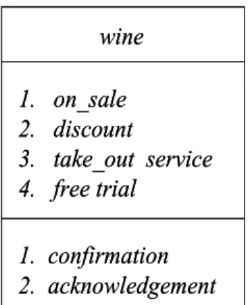
An example for a class “wine” is shown in Figure 2 to illustrate the above concept. The class name is specified as “wine”. The class includes four attributes, on_sale, discount, take_out service, and free trial. It also has two methods, confirmation and acknowledgement.
class name attribute 1 attribute 2 . . . attribute n method 1 method 2 . . . method m message response class name attribute 1 attribute 2 . . . attribute n method 1 method 2 . . . method m message response
wine 1. on_sale 2. discount 3. take_out service 4. free trial 1. confirmation 2. acknowledgement wine 1. on_sale 2. discount 3. take_out service 4. free trial 1. confirmation 2. acknowledgement
Figure 2: An example of the class “wine”
In this paper, each item itself (or item name) is thought of as a class, and each item purchased in a transaction is thought of as an instance. Instances with the same class (item name) may have different quantitative attribute values since they may appear in different transactions.
4. The fuzzy data-mining algorithm for quantitative object-oriented
transaction data
In this section, the fuzzy concepts are used in the proposed algorithm for discovering useful association rules from quantitative objected-oriented transactions. The notation used in the algorithm is first listed below.
Notation:
n: the number of quantitative object-oriented transactions; w: the number of items (classes);
m: the number of attributes for each item;
) (i
D : the i-th quantitative object-oriented transaction, 1in;
Ij: the j-th item (class), 1 j w;
Ak: the k-th attribute, 1 k m;
Ij.Ak: the k-th attribute of the j-th item; k
j A
I . : the number of fuzzy regions for Ij.Ak;
jkl
R : the l-th fuzzy region of Ij.Ak, 1l I . ; jAk
i jk
v : the quantitative value of Ij.Ak inD(i); i
jk
f
: the fuzzy set converted from i jkv ;
) (i jkl
f : the membership value of i jk
v in RegionR ; jkl
jkl
count : the count ofR ; jkl
α: the predefined minimum support value; λ: the predefined minimum confidence value;
Cr: the set of candidate itemsets with r intra-object items; r
L : the set of large itemsets with r intra-object items;
' z
C : the set of candidate itemsets with z inter-object items;
' z
L : the set of large itemsets with z inter-object items.
The proposed fuzzy mining algorithm first uses the defined membership functions to transform the quantitative value of each item attribute in a transaction
into a fuzzy set in linguistic terms. The algorithm then calculates the scalar cardinality of each linguistic term from all the converted object-oriented transactions. The mining process using fuzzy sets is then performed to find fuzzy association rules. The proposed fuzzy algorithm can be divided into two main phases. The first phase is called the fuzzy intra-object mining phase, in which the linguistic large itemsets associated with the same classes (items) but with different attributes are derived. The phase can find out the linguistic association relation within the same kind of objects. Each linguistic large itemset found in this phase can be thought of as a composite item used in phase 2. The second phase is called the fuzzy inter-object mining phase, in which the large itemsets derived from the composite items are used to represent the relationship among different kinds of objects. Both the fuzzy intra-object and fuzzy inter-object association rules can thus be easily derived by the proposed algorithm at the same time. Two apriori-like procedures are adopted to find the two kinds of rules.
The details of the proposed algorithm are described below.
The fuzzy object-oriented data-mining algorithm for association rules:
INPUT: A set of w items (classes) with m quantitative attributes, a body of n
transaction data, each with some items and their attribute values, a set of membership functions, a predefined minimum support value α, and a predefined confidence value λ.
OUTPUT: A set of fuzzy intra- and inter-object association rules. STEP 1: Transform the quantitative value i
jk
v of the i-th transaction datum D(i) for each item attribute Ij.Ak into a fuzzy set fjk i represented as:
jkp i jkp jk i j jk i jk R f R f R f k .... 2 1 ) ( 1 2 ,
using the given membership functions, where i = 1 to n, Ij is the j-th item (class), 1 j w, Ak is the k-th attribute, 1 k m, Rjkl is the l-th fuzzy region of attribute Ij.Ak, fjkl i isv jki ’s fuzzy membership value in regionR , jkl and p is the number of fuzzy regions for Ij.Ak.
STEP 2: Calculate the scalar cardinality of each fuzzy attribute region Rjkl in the transaction data as its count:
n i i jkl jkl f count 1 .STEP 3: Calculate the support of each attribute region Rjkl as:
supportjkl = countjkl / n, where n is the number of transactions.
STEP 4: Check whether the supportjkl of each fuzzy region Rjkl is larger than or equal to the predefined minimum support valueα. If supportjkl is equal to or greater than the minimum support value, put Rjkl in the set of large 1-itemsets (L1). That is,
STEP 5: If L1 is null, then exit the algorithm; otherwise, do the next step.
STEP 6: Set r = 1, where r is the number of items in the itemsets currently being
processed.
STEP 7: Generate the candidate set Cr+1 by joining Lr in a way similar to that in the
apriori algorithm [4] except that the two (r-1)-itemsets to be joined must
have the same classes (items).
STEP 8: Do the following substeps for each newly formed (r+1)-itemset s with items
(s1, s2, …, sr+1) in Cr+1:
(a) Calculate the fuzzy value of s in each transaction data D as: (i) i s i s i s i s f f f r f ( ) 1 2 ... 1 , where (i) sj
f is the membership value of the fuzzy region sj inD(i). If the minimum operator is used for the intersection, then:
i s r j i s Minf j f 1 1 ) ( .
(b) Calculate the scalar cardinality of s in the transaction data as its count: counts =
n i i s f 1 ) ( .(c) Calculate the support of each attribute region Rs as:
supports= counts / n, where n is the number of transactions.
(d) If supports is larger than or equal to the predefined minimum support value , put s in Lr+1.
STEP 9: If Lr+1 is null, then do the next step; otherwise, set r = r + 1 and repeat STEPs 7 and 8.
STEP 10: Each large itemset found so far is then thought of as a fuzzy intra-object composite item and is put in the fuzzy inter-object large 1-itemset ( '
1
L ).
STEP 11: Set z = 1, where z is used to represent the number of fuzzy composite items
in the intra-object itemsets currently being processed. STEP 12: Generate the candidate set '
1 z
C from '
z
L in a way similar to that in the apriori algorithm under the condition that each (z+1)-itemset must not
include fuzzy composite items from the same classes.
STEP 13: Do the following substeps for each newly formed fuzzy (z+1)-itemset s
with items (s1, s2, …, sz+1) in C : z'1
(a) Calculate the fuzzy value of s in each transaction data D as: (i) i s i s i s i s f f f r f ( ) 1 2 ... 1 , where (i) sj
f is the membership value of fuzzy region sj inD(i). If the minimum operator is used for the intersection, then:
. 1 1 ) ( i s z j i s Min f j f
counts =
n i i s f 1 ) ( .(c) Calculate the support of each attribute region Rs as:
supports= counts / n, where n is the number of transactions.
(d) If supports is larger than or equal to the predefined minimum support value α, put s in ' 1 z L . STEP 14: If ' 1 z
L is null, do the next step; otherwise, set z = z +1 and repeat STEPs
12 and 13.
STEP 15: Derive the fuzzy intra-object association rules for any large q-itemset s with
items (s1, s2, …, sq), q2, from the large itemsets L2 to Lr, using the
following substeps:
(a) Form all possible association rules as follows:
s1...st1st1...sq st, t = 1 to q.
(b) Calculate the confidence values of all association rules by:
confs =
n i i s i s i s i s n i i s q t t t f f f f f 1 ) ( ) ( ) ( ) ( 1 ) ( ) ... ... ( 1 1 1 .(c) Output the rules with confidence values larger than or equal to the predefined confidence threshold λ.
than or equal to λ from the large itemsets ' 2 L to ' z L in a way similar to STEP 15.
After STEP 16, the two kinds of fuzzy intra- and inter-object association rules are found from the given set of quantitative object-oriented transactions. These fuzzy rules can thus be used as meta-knowledge to form business decisions.
5. An Example
In this section, an example is given to illustrate the proposed fuzzy data-mining algorithm. This is a simple example to show how the proposed algorithm can be used to generate fuzzy inter-object and intra-object sale strategy for commodities in a store. Assume there are four items, I1 to I4, to be sold in this example and each item has the
same four quantitative attributes, represented as A1 to A4, related to the sale behavior.
For example, the attributes may be quantities and numbers of colors, among others. Also assume the data set includes 10 transactions, as shown in Table 1, where the number for Ij.Ak represents the quantitative value for the attribute Ij.Ak.
Table 1: The set of 10 transactions in the example Transaction
ID
Purchased
Items ID Attribute values of purchased items 1 I1, I3, I4
(I1.A1:6, I1.A2:7, I1.A3:13, I1.A4:9), (I3.A1:1, I3.A2:5,
2 I2, I4 (I2.A1:2, I2.A2:6, I2.A4:10), (I4.A1:1, I4.A3:5, I4.A4:3) 3 I1, I4 (I1.A1:6, I1.A3:11) , (I4.A2:6) 4 I2, I3 (I2.A2:6), (I3.A2:8, I3.A3:1, I3.A4:5) 5 I1, I2 (I1.A1:6, I1.A2:6, I1.A3:15, I1.A4:6), (I2.A1:7, I2.A2:6, I2.A3:4) 6 I1, I4 (I1.A1:6, I1.A2:6, I1.A3:9), (I4.A1:1, I4.A2:3, I4.A3:6) 7 I1, I2, I3, I4 (I1.A1:6, I1.A2:8, I1.A4:5), (I2.A1:5, I2.A2:6, I2.A4:1), (I3.A1:3, I3.A2:7, I3.A3:1), (I4.A2:2) 8 I1, I2, I3, I4 (I1.A1:6, I1.A2:6, I1.A3:6), (I2.A3:13, I2.A4:3), (I3.A1:5, I3.A3:1), (I4.A1:7, I4.A3:6) 9 I1, I2 (I1.A1:7, I1.A3:13), (I2.A3:9) 10 I1, I3, I4 (I1.A1:9, I1.A2:3, I1.A3:10), (I3.A4:5), (I4.A3:6, I4.A4:3)
Assume the fuzzy membership functions for the quantitative attribute values are shown in Figure 3.
Membership value
0 1 6 11 Quantity 1
Low Middle High Membership value
0 1 6 11 Quantity 1
Low Middle High
Figure 3: The membership functions used in this example
In this example, we assume all attributes have the same membership functions for simplicity. Attributes with different membership functions can be managed in a similar way. In Figure 1, each attribute has three fuzzy regions: Low, Middle, and High. Three fuzzy membership values are thus produced for each attribute according
to the predefined membership functions. For the transaction data in Table 1, the proposed fuzzy mining algorithm proceeds as follows.
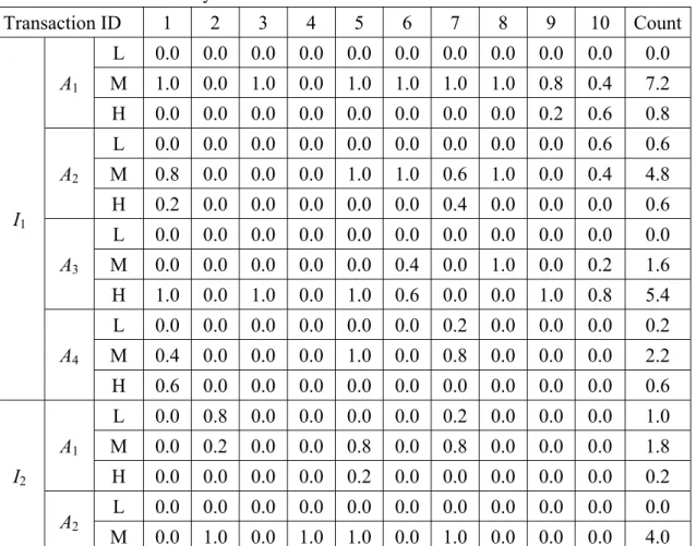
STEP 1: The quantitative values of each item attribute in each transaction datum are transformed into fuzzy sets. Take the item attribute I1.A2 in the first
transaction as an example. The value of the attribute A2 in Item I1 is 7, and is
converted into a fuzzy set (0.0/Low + 0.8/Middle + 0.2/High)using the given membership functions. This step is repeated for the other transactions and item attributes, with the results shown in Table 2.
Table 2: The fuzzy sets of the item attributes transformed from Table 1
Transaction ID 1 2 3 4 5 6 7 8 9 10 Count I1 A1 L 0.0 0.0 0.0 0.0 0.0 0.0 0.0 0.0 0.0 0.0 0.0 M 1.0 0.0 1.0 0.0 1.0 1.0 1.0 1.0 0.8 0.4 7.2 H 0.0 0.0 0.0 0.0 0.0 0.0 0.0 0.0 0.2 0.6 0.8 A2 L 0.0 0.0 0.0 0.0 0.0 0.0 0.0 0.0 0.0 0.6 0.6 M 0.8 0.0 0.0 0.0 1.0 1.0 0.6 1.0 0.0 0.4 4.8 H 0.2 0.0 0.0 0.0 0.0 0.0 0.4 0.0 0.0 0.0 0.6 A3 L 0.0 0.0 0.0 0.0 0.0 0.0 0.0 0.0 0.0 0.0 0.0 M 0.0 0.0 0.0 0.0 0.0 0.4 0.0 1.0 0.0 0.2 1.6 H 1.0 0.0 1.0 0.0 1.0 0.6 0.0 0.0 1.0 0.8 5.4 A4 L 0.0 0.0 0.0 0.0 0.0 0.0 0.2 0.0 0.0 0.0 0.2 M 0.4 0.0 0.0 0.0 1.0 0.0 0.8 0.0 0.0 0.0 2.2 H 0.6 0.0 0.0 0.0 0.0 0.0 0.0 0.0 0.0 0.0 0.6 I2 A1 L 0.0 0.8 0.0 0.0 0.0 0.0 0.2 0.0 0.0 0.0 1.0 M 0.0 0.2 0.0 0.0 0.8 0.0 0.8 0.0 0.0 0.0 1.8 H 0.0 0.0 0.0 0.0 0.2 0.0 0.0 0.0 0.0 0.0 0.2 A2 L 0.0 0.0 0.0 0.0 0.0 0.0 0.0 0.0 0.0 0.0 0.0 M 0.0 1.0 0.0 1.0 1.0 0.0 1.0 0.0 0.0 0.0 4.0
H 0.0 0.0 0.0 0.0 0.0 0.0 0.0 0.0 0.0 0.0 0.0 A3 L 0.0 0.0 0.0 0.0 0.4 0.0 0.0 0.0 0.0 0.0 0.4 M 0.0 0.0 0.0 0.0 0.6 0.0 0.0 0.0 0.4 0.0 1.0 H 0.0 0.0 0.0 0.0 0.0 0.0 0.0 1 0.6 0.0 1.6 A4 L 0.0 0.0 0.0 0.0 0.0 0.0 1 0.6 0.0 0.0 1.6 M 0.0 0.2 0.0 0.0 0.0 0.0 0.0 0.4 0.0 0.0 0.6 H 0.0 0.8 0.0 0.0 0.0 0.0 0.0 0.0 0.0 0.0 0.8 I3 A1 L 1.0 0.0 0.0 0.0 0.0 0.0 0.6 0.2 0.0 0.0 1.8 M 0.0 0.0 0.0 0.0 0.0 0.0 0.4 0.8 0.0 0.0 1.2 H 0.0 0.0 0.0 0.0 0.0 0.0 0.0 0.0 0.0 0.0 0.0 A2 L 0.2 0.0 0.0 0.0 0.0 0.0 0.0 0.0 0.0 0.0 0.2 M 0.8 0.0 0.0 0.6 0.0 0.0 0.8 0.0 0.0 0.0 2.2 H 0.0 0.0 0.0 0.4 0.0 0.0 0.2 0.0 0.0 0.0 0.6 A3 L 0.0 0.0 0.0 1.0 0.0 0.0 1.0 1.0 0.0 0.0 3.0 M 0.4 0.0 0.0 0.0 0.0 0.0 0.0 0.0 0.0 0.0 0.4 H 0.6 0.0 0.0 0.0 0.0 0.0 0.0 0.0 0.0 0.0 0.6 A4 L 0.0 0.0 0.0 0.2 0.0 0.0 0.0 0.0 0.0 0.2 0.4 M 0.0 0.0 0.0 0.8 0.0 0.0 0.0 0.0 0.0 0.8 1.6 H 0.0 0.0 0.0 0.0 0.0 0.0 0.0 0.0 0.0 0.0 0.0 I4 A1 L 1.0 1.0 0.0 0.0 0.0 1.0 0.0 0.0 0.0 0.0 3.0 M 0.0 0.0 0.0 0.0 0.0 0.0 0.0 0.8 0.0 0.0 0.8 H 0.0 0.0 0.0 0.0 0.0 0.0 0.0 0.2 0.0 0.0 0.2 A2 L 0.0 0.0 0.0 0.0 0.0 0.6 0.8 0.0 0.0 0.0 1.4 M 0.0 0.0 1.0 0.0 0.0 0.4 0.2 0.0 0.0 0.0 1.6 H 0.0 0.0 0.0 0.0 0.0 0.0 0.0 0.0 0.0 0.0 0.0 A3 L 0.0 0.2 0.0 0.0 0.0 0.0 0.0 0.0 0.0 0.0 0.2 M 0.8 0.8 0.0 0.0 0.0 1.0 0.0 1.0 0.0 1.0 4.6 H 0.2 0.0 0.0 0.0 0.0 0.0 0.0 0.0 0.0 0.0 0.2 A4 L 0.0 0.6 0.0 0.0 0.0 0.0 0.0 0.0 0.0 0.6 1.2 M 0.0 0.4 0.0 0.0 0.0 0.0 0.0 0.0 0.0 0.4 0.8 H 0.0 0.0 0.0 0.0 0.0 0.0 0.0 0.0 0.0 0.0 0.0
STEP 2: The scalar cardinality of each fuzzy attribute region in the transactions is calculated as the count value. Take the region I1.A2.Middle as an example.
repeated for the other regions, with the results shown in the right column of Table 2.
STEP 3: The support of each fuzzy region is calculated as its count divided by 10.
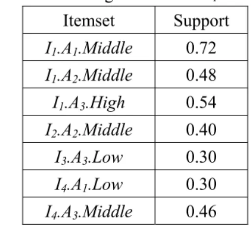
STEP 4: The support of each fuzzy region is then checked against the predefined minimum support value α. Assume in this example, α is set at 25%. Since the support values of I1.A1.Middle, I1.A2.Middle, I1.A3.High, I2.A2.Middle,
I3.A3.Low, I4.A1.Low and I4.A3.Middle are larger than 0.25, these fuzzy regions are thus put in L1 (Table 3).
Table 3: The set of large 1-itemsets L1 for this example
Itemset Support I1.A1.Middle 0.72 I1.A2.Middle 0.48 I1.A3.High 0.54 I2.A2.Middle 0.40 I3.A3.Low 0.30 I4.A1.Low 0.30 I4.A3.Middle 0.46
STEP 5: If L1 is null, then the algorithm is exited; otherwise, the next step is done. In this example, since L1 is not null, STEP 6 is then executed.
being processed.
STEP 7: The candidate set Cr+1 is formed by joining Lr and Lr such that the two (r-1)-itemsets to be joined must have the same items (classes). C2 is first
generated from L1 as follows: (I1.A1.Middle, I1.A2.Middle), (I1.A1.Middle,
I1.A3.High), (I1.A2.Middle, I1.A3.High) and (I4.A1.Low, I4.A3.Middle).
STEP 8: The following substeps is executed for each newly formed candidate itemset.
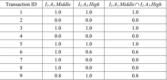
(a) The fuzzy membership value of a candidate itemset in each transaction datum is calculated. Here, the minimum operator is used for the intersection. Take (I1.A1.Middle, I1.A3.High) as an example. The derived membership value for the tenth transaction is calculated as: min(0.4, 0.8) =
0.4. The results for all the transactions are shown in Table 4.
Table 4: The membership values for (I1.A1.MiddleI1.A3.High) Transaction ID I1.A1.Middle I1.A3.High I1.A1.MiddleI1.A3.High
1 1.0 1.0 1.0 2 0.0 0.0 0.0 3 1.0 1.0 1.0 4 0.0 0.0 0.0 5 1.0 1.0 1.0 6 1.0 0.6 0.6 7 1.0 0.0 0.0 8 1.0 0.0 0.0 9 0.8 1.0 0.8
10 0.4 0.8 0.4
The results for the other candidate 2-itemsets can be derived in a similar fashion.
(b) The scalar cardinality (count) of each candidate 2-itemset is found from the transactions. Results for this example are shown in Table 5.
Table 5: The fuzzy counts of the itemsets in C2
Itemset Count (I1.A1.Middle, I1.A2.Middle) 4.8
(I1.A1.Middle, I1.A3.High) 4.8 (I1.A2.Middle, I1.A3.High) 2.8 (I4.A1.Low, I4.A3.Middle) 2.6
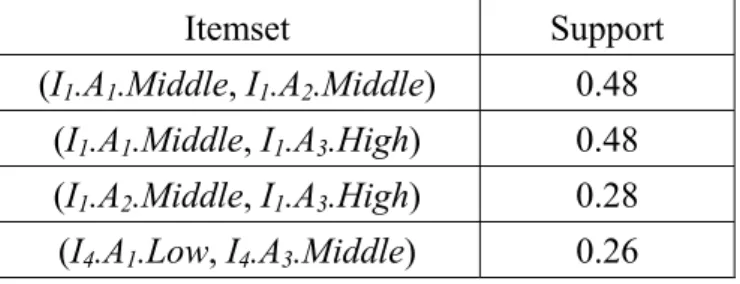
(c) The support of each itemset in C2 is calculated as its count divided by 10. (d) The supports are then checked against the predefined minimum support
value 25%. In this example, the four 2-itemsets, (I1.A1.Middle,
I1.A2.Middle), (I1.A1.Middle, I1.A3.High), (I1.A2.Middle, I1.A3.High) and (I4.A1.Low, I4.A3.Middle) are large and kept in L2 (Table 6).
Table 6: The large itemsets and their supports in L2
Itemset Support (I1.A1.Middle, I1.A2.Middle) 0.48
(I1.A1.Middle, I1.A3.High) 0.48
(I1.A2.Middle, I1.A3.High) 0.28
STEP 9: IF Lr+1 is null, the next step is done; otherwise, r = r + 1 and STEPs 7 to 8 are repeated. Since L2 is not null in the example, r = r + 1 = 2. STEPs 7 to 8 are then repeated to find L3. C3 is first generated from L2, and only the 3-itemset (I1.A1.Middle, I1.A2.Middle, I1.A3.High) is formed. Its support is calculated as 0.28, larger than 0.25. It is thus put in L3. Since L3 contains only one itemset, no 4-itemsets are formed and L4 is null. STEP 10 then
begins.
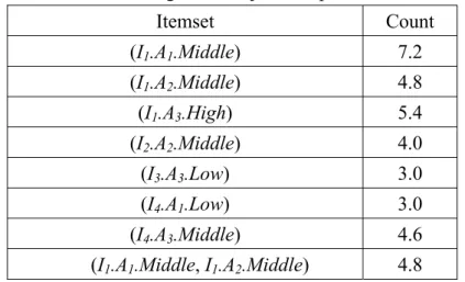
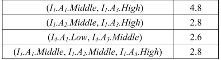
STEP 10: Each large itemset found so far is thought of as a fuzzy intra-object composite item and is put in the fuzzy inter-object large 1-itemset ( '
1
L). In
this example, the large itemsets (I1.A1), (I1.A2), (I1.A3), (I2.A2), (I3.A3), (I4.A1),
(I4.A3), (I1.A1, I1.A2), (I1.A1, I1.A3), (I1.A2, I1.A3), (I4.A1, I4.A3), (I1.A1, I1.A2,
I1.A3) are put in the set of largeL . Table 7 shows the results. '1
Table 7: The set of large inter-object composite 1-itemsets ' 1 L Itemset Count (I1.A1.Middle) 7.2 (I1.A2.Middle) 4.8 (I1.A3.High) 5.4 (I2.A2.Middle) 4.0 (I3.A3.Low) 3.0 (I4.A1.Low) 3.0 (I4.A3.Middle) 4.6 (I1.A1.Middle, I1.A2.Middle) 4.8
(I1.A1.Middle, I1.A3.High) 4.8
(I1.A2.Middle, I1.A3.High) 2.8
(I4.A1.Low, I4.A3.Middle) 2.6
(I1.A1.Middle, I1.A2.Middle, I1.A3.High) 2.8
STEP 11: z is set at 1, where z is used to represent the number of composite items in
the intra-object itemsets currently being processed.
STEP 12: The candidate set ' 1 z C is generated by joining ' z L and ' z L under the
condition that each (z+1)-itemset must not include composite items from
the same classes. ' 2
C is first generated from .' 1
L There are totally forty-two
candidates generated in ' 2
C .
STEP 13: The following substeps are executed for each newly formed candidate itemset.
(a) The fuzzy membership value of a candidate itemset in each transaction is calculated.
(b) The scalar cardinality (count) of each candidate 2-itemset in the transaction data is calculated. Results for this example are shown in Table 8.
Table 8: The counts of the itemsets in ' 2
C
[(I1.A1.Middle), (I2.A2.Middle)] 2.0 [(I2.A2.Middle), (I4.A1.Low, I4.A3.Middle)] 0.8 [(I1.A1.Middle), (I3.A3.Low)] 2.0 [(I2.A2.Middle), (I1.A1.Middle, I1.A2.Middle, I1.A3.High)] 1.0 [(I1.A1.Middle), (I4.A1.Low)] 2.0 [(I3.A3.Low), (I4.A1.Low)] 0.0 [(I1.A1.Middle), (I4.A3.Middle)] 3.2 [(I3.A3.Low), (I4.A3.Middle)] 1.0
[(I1.A1.Middle), (I4.A1.Low, I4.A3.Middle)] 1.8 [(I3.A3.Low), (I1.A1.Middle, I1.A2.Middle)] 1.6 [(I1.A2.Middle), (I2.A2.Middle)] 1.6 [(I3.A3.Low), (I1.A1.Middle, I1.A3.High)] 0.0 [(I1.A2.Middle), (I3.A3.Low)] 1.6 [(I3.A3.Low), (I1.A2.Middle, I1.A3.High)] 0.0 [(I1.A2.Middle), (I4.A1.Low)] 1.8 [(I3.A3.Low), (I4.A1.Low, I4.A3.Middle)] 0.0 [(I1.A2.Middle), (I4.A3.Middle)] 3.2 [(I3.A3.Low), (I1.A1.Middle, I1.A2.Middle, I1.A3.High)] 0.0 [(I1.A2.Middle), (I4.A1.Low, I4.A3.Middle)] 1.8 [(I4.A1.Low), (I1.A1.Middle, I1.A2.Middle)] 1.8 [(I1.A3.High), (I2.A2.Middle)] 1.0 [(I4.A1.Low), (I1.A1.Middle, I1.A3.High)] 1.6 [(I1.A3.High), (I3.A3.Low)] 0.0 [(I4.A1.Low), (I1.A2.Middle, I1.A3.High)] 1.4 [(I1.A3.High), (I4.A1.Low)] 1.6 [(I4.A1.Low), (I1.A1.Middle, I1.A2.Middle, I1.A3.High)] 1.4 [(I1.A3.High), (I4.A3.Middle)] 2.2 [(I4.A3.Middle), (I1.A1.Middle, I1.A2.Middle)] 3.2 [(I1.A3.High), (I4.A1.Low, I4.A3.Middle)] 1.4 [(I4.A3.Middle), (I1.A1.Middle, I1.A3.High)] 1.8 [(I2.A2.Middle), (I3.A3.Low)] 2.0 [(I4.A3.Middle), (I1.A2.Middle, I1.A3.High)] 1.8 [(I2.A2.Middle), (I4.A1.Low)] 1.0 [(I4.A3.Middle), (I1.A1.Middle, I1.A2.Middle, I1.A3.High)] 1.8 [(I2.A2.Middle), (I4.A3.Middle)] 0.8 [(I1.A1.Middle, I1.A2.Middle), (I4.A1.Low, I4.A3.Middle)] 1.8 [(I2.A2.Middle), (I1.A1.Middle, I1.A2.Middle)] 1.6 [(I1.A1.Middle, I1.A3.High), (I4.A1.Low, I4.A3.Middle)] 1.4 [(I2.A2.Middle), (I1.A1.Middle, I1.A3.High)] 1.0 [(I1.A2.Middle, I1.A3.High), (I4.A1.Low, I4.A3.Middle)] 1.4
[(I2.A2.Middle), (I1.A2.Middle, I1.A3.High)] 1.0 [(I4.A1.Low, I4.A3.Middle), (I1.A1.Middle, I1.A2.Middle, I1.A3.High)] 1.4
(c) The support of each fuzzy region is calculated as its count divided by 10. (d) These supports are then checked against the predefined minimum support
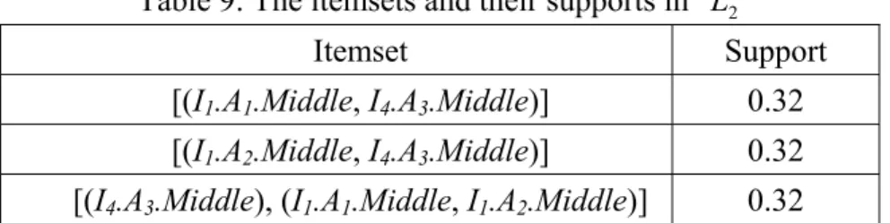
value 2.5. In this example, the four itemsets, [(I1.A1.Middle), (I4.A3.Middle)], [(I1.A2.Middle), (I4.A3.Middle)], [(I1.A3.High), (I4.A3.Middle)] and [(I4.A3.Middle), (I1.A1.Middle, I1.A2.Middle)] are large and kept in L2 (Table 9).
Table 9: The itemsets and their supports in ' 2
L
Itemset Support
[(I1.A1.Middle, I4.A3.Middle)] 0.32
[(I1.A2.Middle, I4.A3.Middle)] 0.32
[(I4.A3.Middle), (I1.A1.Middle, I1.A2.Middle)] 0.32
STEP 14: If ' 1 z
L is null, the next step is done; otherwise, z = z + 1 and STEPs 12 to
13 are repeated. Since ' 2
L is not null in the example, z = z + 1 = 2. STEPs
12 to 13 are then repeated to find ' 3
L . ' 3
C is first generated from ' 2
L . In
this example ' 3
C is empty. STEP 15 then begins.
STEP 15: Fuzzy intra-object association rules with confidence values larger than or equal to the minimum confidence value λ are derived from the large itemsets
The following eleven rules are derived and output to users:
1. “If I1.A1 = Middle, then I1.A2 = Middle” with a confidence factor of 0.67; 2. “If I1.A2 = Middle, then I1.A1 = Middle” with a confidence factor of 1; 3. “If I1.A1 = Middle, then I1.A3 = High” with a confidence factor of 0.67; 4. “If I1.A3 = High, then I1.A1 = Middle” with a confidence factor of 0.89; 5. “If I1.A2 = Middle, then I1.A3 = High” with a confidence factor of 0.58; 6. “If I4.A1 = Low, then I4.A3 = Middle” with a confidence factor of 0.87; 7. “If I4.A3 = Middle, then I4.A1 = Low” with a confidence factor of 0.57; 8. “If (I1.A2 = Middle and I1.A3 = High), then I1.A1 = Middle” with a
confidence factor of 1;
9. “If I1.A2 = Middle, then (I1.A1 = Middle and I1.A3 = High)” with a confidence factor of 0.58;
10. “If (I1.A1 = Middle and I1.A3 = High), then I1.A2 = Middle” with a confidence factor of 0.58;
11. “If (I1.A1 = Middle and I1.A2 = Middle), then I1.A3 = High” with a confidence factor of 0.58.
The above rules can then be explained in a comprehensible way. For example, the association rule "If (I1.A2 = Middle and I1.A3 = High), then I1.A1 = Middle" with a
confidence factor of 1 can be explained as “If item I1 has a middle amount of A2
values and a high amount of A3 values, thenI1 will also have a middle amount of A1
values” with a confidence factor of 1.
STEP 16: Fuzzy inter-object association rules with confidence values larger than or equal to λ are derived from the large itemsets '
2
L to ' z
L . In this example, z = 2. The following fuzzy inter-object association rules are thus derived:
1. "If I4.A3 = Middle, then I1.A1 = Middle " with a confidence factor of 0.7; 2. "If I1.A2 = Middle, then I4.A3 = Middle " with a confidence factor of
0.67;
3. "If I4.A3 = Middle, then I1.A2 = Middle " with a confidence factor of 0.7; 4. "If (I1.A1 = Middle and I1.A2 = Middle), then I4.A3 = Middle " with a
confidence factor of 0.67;
5. "If I4.A3 = Middle, then (I1.A1 = Middle and I1.A2 = Middle)" with a confidence factor of 0.7;
The association rule "If I4.A3 = Middle, then (I1.A1 = Middle and I1.A2 = Middle)" with a confidence factor of 0.7 can be explained as “If item I4 has a middle amount of
A2 values” with a confidence factor of 0.7.
After STEP 16, the two kinds of fuzzy intra- and inter-object association rules are found from the given set of quantitative object-oriented transactions.
6. Experimental Results
The section reports on experiments made to show the effects of the parameters on the proposed algorithm for fuzzy inter- and intra-object association rules. They were implemented in JAVA on a Pentium-IV 2.8GHz personal computer with 1 GB memory. There were 50 object-oriented items, and each item had three quantitative attributes. Assume the same set of membership functions shown in Figure 3 is used in the experiments. Data sets with different numbers of transactions were run by the proposed algorithm. In each data set, numbers of purchased items in transactions were first randomly generated. The purchased items and their quantitative attribute values in each transaction were then generated. An item could not be generated twice in a transaction.
Experiments were first performed to find the relationships between numbers of rules and minimum supports when the minimum transaction number was set at 2000, the minimum confidence was 0.2, and the average number of purchased items in
transactions was 10. The results for both kinds of the fuzzy intra and inter-object association rules are shown in Figure 4.
0 1000 2000 3000 4000 5000 6000 7000 0.02 0.03 0.04 0.05 0.06 0.07 0.08 0.09 0.1 Minimum support N u m b er o f ru le s
Fuzzy Intra-OO Rules Fuzzy Inter-OO Rules
Figure 4. The relationship between numbers of rules and minimum support values
It can be observed from Figure 4 that the number of rules decreased along with the increase of the minimum support value. It was consistent with the property of data mining. Besides, the numbers of fuzzy intra-object association rules were smaller than those of fuzzy inter-object association rules because the attribute number is less than the item number in the experiments. This situation usually occurs in real applications. Fuzzy intra-object association rules are just internal relations within objects and fuzzy inter-object association rules are external relations among objects. We also find that the execution time for fuzzy intra-object association rules was smaller than that for fuzzy inter-object association rules (which will be shown later).
Figure 5 shows a comparison of the numbers of different large itemsets for fuzzy intra-object association rules along with minimum support values. It can be observed that most of the large itemsets were 1-itemsets, 2-itemsets and 3-itemsets. This was because only three attributes were used in each transaction. It can also be found that curve for L1 was more stable than that for L2.
0 50 100 150 200 250 300 350 400 450 500 0.02 0.03 0.04 0.05 0.06 0.07 0.08 0.09 0.1 Minimum support N u m b er o f la rg e it em set s L1 L2 L3 Total
Figure 5. A comparison of different fuzzy intra-object large itemsets along with minimum supports.
Figure 6 then shows a comparison of the numbers of different inter-object large itemsets along with minimum support values. It can also be found that the curve for L1 was more stable than that for L2. When the minimum support was smaller, the number of large 2-itemsets would increase more sharply.
0 1000 2000 3000 4000 5000 6000 0.02 0.03 0.04 0.05 0.06 0.07 0.08 0.09 0.1 Minimum support N u m b er o f la rg e it em set s L1' L2' L3' Total
Figure 6. A comparison of different fuzzy inter-object large itemsets with minimum supports
Experiments were then made to find the relationships between numbers of rules and minimum confidences when the minimum transaction number was 2000, the minimum support was 0.05 and the average number of purchased items in transactions was 10. The results for both kinds of fuzzy intra- and inter-object association rules are shown in Figure 7.
0 100 200 300 400 500 600 700 800 900 1000 0.2 0.25 0.3 0.35 0.4 0.45 Minimum confidence N u m b er o f ru le s
Fuzzy Intra-OO Rules Fuzzy Inter-OO Rules
Figure 7. The relationship between numbers of rules and minimum confidence values
It can be observed from Figure 7 that the number of rules decreased along with the increase of the minimum confidence value. It was also consistent with the property of data mining. Besides, the numbers of fuzzy intra-object association rules were smaller than those of fuzzy inter-object association rules when the minimum confidence was small. This was because the fuzzy inter-object association rules were derived from the given set of items, which were more than the set of attributes. When the minimum confidence value was high, only a few fuzzy inter-object association rules could be derived.
Experiments were then performed to compare the results of different numbers of transactions. The relationship between numbers of fuzzy intra-object association rules and minimum support values along with different numbers of transactions for an
average of 10 purchased items in a transaction and a minimum confidence value set at 0.2 is shown in Figure 8. The relationship between numbers of fuzzy inter-object association rules and minimum support values along with different numbers of transactions is shown is Figure 9.
0
500
1000
1500
0.01
0.02
0.03
0.04
0.05
Minimum support Nu mb er o f r ul es2000-Fuzzy Intra-OO Rules 4000-Fuzzy Intra-OO Rules 6000-Fuzzy Intra-OO Rules 8000-Fuzzy Intra-OO Rules 10000-Fuzzy Intra-OO Rules
Figure 8. The relationship between numbers of fuzzy intra-object rules and minimum support values for different numbers of transactions
0
500
1000
1500
2000
0.01
0.02
0.03
0.04
0.05
Minimum support
Nu
m
be
r o
f r
ul
es
2000-Fuzzy Inter-OO Rules 4000-Fuzzy Inter-OO Rules 6000-Fuzzy Inter-OO Rules 8000-Fuzzy Inter-OO Rules 10000-Fuzzy Inter-OO Rules
Figure 9. The relationship between numbers of fuzzy inter-object rules and minimum support values for different numbers of transactions
From Figures 8 and 9, it is easily seen that the numbers of rules are nearly the same for different transactions since the minimum support and the minimum confidence were set as ratios and independent of transaction numbers.
At last, the execution time for fuzzy intra-object rules with different minimum support values along with different numbers of transactions for an average of 10 purchased items in transactions and a minimum confidence value set at 0.2 is shown in Figure 10. The execution time for fuzzy inter-object rules is shown in Figure 11. The relationship between execution times and transactions when the support value set
at 0.01 is shown in Figure 12. It is obvious from Figures 10, 11 and 12 that the execution time increased along with the increase of transaction numbers. Besides, finding inter-object association rules spent more time than finding intra-object association rules. This was because the number of items was usually larger than that of the attributes. The second phase is thus the bottleneck of the proposed algorithm.
0
200
400
600
800
0.01
0.02
0.03
0.04
0.05
Minimum support Tim e ( S ec .)2000-Fuzzy Intra-OO Rules 4000-Fuzzy Intra-OO Rules 6000-Fuzzy Intra-OO Rules 8000-Fuzzy Intra-OO Rules 10000-Fuzzy Intra-OO Rules
0
1000
2000
3000
4000
5000
6000
7000
8000
0.01
0.02
0.03
0.04
0.05
Minimum support T im e ( S ec .)2000-Fuzzy Inter-OO Rules 4000-Fuzzy Inter-OO Rules 6000-Fuzzy Inter-OO Rules
8000-Fuzzy Inter-OO Rules 10000-Fuzzy Inter-OO Rules
Figure 11. The execution times for fuzzy inter-object association rules
0
2000
4000
6000
8000
2000
4000
6000
8000
10000
Transactions
T
im
e (S
ec.
)
Fuzzy Intra-OO
Fuzzy Inter-OO
Figure 12. The relationship between execution times and transactions
7. Conclusion and future work
interesting knowledge from object-oriented quantitative transactions. The proposed fuzzy algorithm is divided into two main phases. The first phase is called the fuzzy intra-object mining phase, in which the linguistic large itemsets associated with the same classes (items) but with different attributes are derived. The second phase is called the fuzzy inter-object mining phase, in which the large itemsets derived from the composite items are used to represent the relationship among different kinds of objects. Both the intra-object and inter-object association rules can thus be easily derived by the proposed algorithm at the same time. An example has also been given to illustrate the algorithm in detail. Experimental results have shown the effects of the parameters on the proposed algorithm. The numbers of fuzzy intra-object association rules are usually smaller than those of fuzzy inter-object association rules because the attribute number is less than the item number in real applications. Finding inter-object association rules thus spends more time than finding intra-object association rules. In the future, we will further generalize our approach to manage other different mining problems.
References
[1] R. Agrawal, T. Imielinksi and A. Swami, “Mining association rules between sets of items in large database,“ The 1993 ACM SIGMOD International Conference on
Management of Data, Vol. 22, 1993, pp. 207-216.
[2] R. Agrawal, T. Imielinksi and A. Swami, “Database mining: a performance perspective,” IEEE Transactions on Knowledge and Data Engineering, Vol. 5, No.
6, 1993, pp. 914-925.
[3] R. Agrawal, R. Srikant: “Mining Sequential Patterns”, The Eleventh International Conference on Data Engineering, 1995, pp. 3-14.
[4] R. Agrawal and R. Srikant, “Fast algorithm for mining association rules,” The International Conference on Very Large Databases, 1994, pp. 487-499.
[5] A. F. Blishun, “Fuzzy learning models in expert systems,” Fuzzy Sets and Systems,
Vol. 22, 1987, pp. 57-70.
[6]C. H. Cai, W. C. Fu, C. H. Cheng and W. W. Kwong, “Mining association rules with weighted items,” The International Database Engineering and Applications Symposium, 1998, pp. 68-77.
[7] L. M. de Campos and S. Moral, “Learning rules for a fuzzy inference model,”
Fuzzy Sets and Systems, Vol. 59, 1993, pp. 247-257.
[8] R. L. P. Chang and T. Pavliddis, “Fuzzy decision tree algorithms,” IEEE Transactions on Systems, Man and Cybernetics, Vol. 7, 1977, pp. 28-35.
[9] C. Clair, C. Liu and N. Pissinou, “Attribute weighting: a method of applying domain knowledge in the decision tree process,” The Seventh International
Conference on Information and Knowledge Management, 1998, pp. 259-266.
[10] P. Clark and T. Niblett, “The CN2 induction algorithm,” Machine Learning, Vol.
3, 1989, pp. 261-283.
[11] M. Delgado and A. Gonzalez, “An inductive learning procedure to identify fuzzy systems,” Fuzzy Sets and Systems, Vol. 55, 1993, pp. 121-132.
[12] A. Famili, W. M. Shen, R. Weber and E. Simoudis, "Data preprocessing and intelligent data analysis," Intelligent Data Analysis, Vol. 1, No. 1, 1997.
[13] W. J. Frawley, G. Piatetsky-Shapiro and C. J. Matheus, “Knowledge discovery in databases: an overview,” The AAAI Workshop on Knowledge Discovery in Databases, 1991, pp. 1-27.
[14] T. Fukuda, Y. Morimoto, S. Morishita and T. Tokuyama, "Mining optimized association rules for numeric attributes," The ACM SIGACT-SIGMOD-SIGART Symposium on Principles of Database Systems, June 1996, pp. 182-191.
[15] A. Gonzalez, “A learning methodology in uncertain and imprecise environments,” International Journal of Intelligent Systems, Vol. 10, 1995, pp.
57-371.
[16] I. Graham and P. L. Jones, Expert Systems – Knowledge, Uncertainty and Decision, Chapman and Computing, Boston, 1988, pp.117-158.
functions," Fuzzy Sets and Systems, Vol.103, No. 3, 1999, pp. 389-404.
[18] T. P. Hong and J. B. Chen, "Processing individual fuzzy attributes for fuzzy rule induction," Fuzzy Sets and Systems, Vol. 112, No. 1, 2000, pp. 127-140.
[19] T. P. Hong, C. S. Kuo and S. C. Chi, "A data mining algorithm for transaction data with quantitative values," Intelligent Data Analysis, Vol. 3, No. 5, 1999, pp. 363-376.
[20] T. P. Hong and C. Y. Lee, "Induction of fuzzy rules and membership functions from training examples," Fuzzy Sets and Systems, Vol. 84, 1996, pp. 33-47.
[21] T. P. Hong and S. S. Tseng, “A generalized version space learning algorithm for noisy and uncertain data,” IEEE Transactions on Knowledge and Data
Engineering, Vol. 9, No. 2, 1997, pp. 336-340.
[22] R. H. Hou, T. P. Hong, S. S. Tseng and S. Y. Kuo, “A new probabilistic induction method, ” Journal of Automatic Reasoning, Vol. 18, 1997, pp. 5-24.
[23] A. Kandel, Fuzzy Expert Systems, CRC Press, Boca Raton, 1992, pp. 8-19.
[24] T. D. Kimura, “Object-oriented dataflow,” The Eleventh IEEE International Symposium on Visual Languages, 1995, pp. 180 – 186.
[25] E. H. Mamdani, “Applications of fuzzy algorithms for control of simple dynamic plants, “ IEEE Proceedings, 1974, pp. 1585-1588.
Conference on Database Theory, 1997.
[27] J. R. Quinlan, “Decision tree as probabilistic classifier,” The Fourth International Machine Learning Workshop, Morgan Kaufmann, San Mateo, CA,
1987, pp. 31-37.
[28] J. R. Quinlan, C4.5: Programs for Machine Learning, Morgan Kaufmann, San
Mateo, CA, 1993.
[29]R. Rastogi and K. Shim, "Mining optimized support rules for numeric attributes," The 15th IEEE International Conference on Data Engineering, Sydney, Australia, 1999, pp. 206-215.
[30] J. Rives, “FID3: fuzzy induction decision tree,” The First International symposium on Uncertainty, Modeling and Analysis, 1990, pp. 457-462.
[31]R. Srikant and R. Agrawal, “Mining generalized association rules,” in Proceeding of the 21st International Conference on Very Large Data Bases, pp. 407-419, 1995.
[32] R. Srikant and R. Agrawal, “Mining quantitative association rules in large relational tables,” The 1996 ACM SIGMOD International Conference on Management of Data, Monreal, Canada, June 1996, pp. 1-12.
[33] R. Srikant, Q. Vu and R. Agrawal, “Mining association rules with item constraints,” The Third International Conference on Knowledge Discovery in
Databases and Data Mining, Newport Beach, California, August 1997,
pp.67-73.
[34] C. H. Wang, T. P. Hong and S. S. Tseng, “Inductive learning from fuzzy examples,” The Fifth IEEE International Conference on Fuzzy Systems, New
Orleans, 1996, pp. 13-18.
[35] C. H. Wang, J. F. Liu, T. P. Hong and S. S. Tseng, “A fuzzy inductive learning strategy for modular rules,” Fuzzy Sets and Systems, Vol.103, No. 1, 1999, pp.
91-105.
[36] R. Weber, “Fuzzy-ID3: a class of methods for automatic knowledge acquisition,”
The Second International Conference on Fuzzy Logic and Neural Networks,
Japan, 1992, pp. 265-268.
[37] K. Won, “Object-oriented databases: definition and research directions,” IEEE Transactions on Knowledge and Data Engineering, Vol. 2, No. 3, 1990, pp.
327-341.
[38] Y. Yuan and M. J. Shaw, “Induction of fuzzy decision trees,” Fuzzy Sets and Systems, 69, 1995, pp. 125-139.
[39] S. Yue, E. Tsang, D. Yeung and D. Shi, “Mining fuzzy association rules with weighted items,” The IEEE International Conference on Systems, Man and Cybernetics, 2000, pp. 1906-1911.
[40] L. A. Zadeh, “Fuzzy logic,” IEEE Computer, 1988, pp. 83-93.
[41] L. A. Zadeh, “Fuzzy sets,” Information and Control, Vol. 8, No. 3, 1965, pp.