The topographic mapping of EEG using the first positive Lyapunov exponent

(1)

1995 IEEE-EMBC and CMBEC

The Topographic Mapping of

EEG

Using

the First Positive Lyapunov Exponent

Theme 4: Signal Processing

Yue-Der Lin*

,

Fok-Ching Chong* , Shing-Ming Sung, Te-Son Kuo*

*

Department

of Electrical Engineering,National

Taiwan

University

Department of Neurology,Taipei Municipal Jen-Ai Hospital

ABSTRACT

ElectroencepNog”@EG) signal is known

to be chaotic and bas the CharactaiStics of un-

predictability. Dimensional analysis of a chaotic signal is an important index to quantify and qualify its dynamical characteristics. The first positive Lyapunov exponent is one of the dim-

ensional analysis and is a standard method of checking whether a time series is chaotic or not. Here we present a new method to derive the topographic mapping of EEG. Using the

f

k

t

positive Lyapunov exponent

,

the derived mapping shows the chaotic state at each site of cerebral cortex which would be important for neurophy- siologists and psychologists

.

Keywords : E l e c t r o e n c e p h a l o g G )

,

the

first positive Lyapunov exponent

,

topographic mapping

INTRODUCTION

The rationale for topographic mapping is that the traditional EEG or evoked potential (EP) tra- cings contain information which under circums- tances

,

is not appreciated by the naked eyes. To- pographic mapping can be viewed as a novel approach to clinical neurophysiology

,

to complent rather

than

replace the many time- proven visual analytical techniques[l]. The

usual

methods to derive the mapping

are

to record

EEG

signals by

a

set of uniformly distributed scalp electrodes , say 16 or more, according to the international 10-20 system at first, and then construct the mapping by the inteqolation procedure with the voltage amplitude at continuous time being interested in or with the power values at certain bands such as alpha (8-13 Hz)

,

th- (4-7

Hz)

or else. The popular interpolation methods are the three and four nearest neighbors (4“) linear algorithm or nonlinear curve-fitting methods using quadratic

or highex order equations. The method

of

interpolation used in map construction have a significant influence on the final appearance.

Since the mid 1980s

,

the development of nonlinear dynamics, or chaos as it is commonly called, has attracted much attention on the appli- cation to physiology. The dimensional analysis of EEG is a revealing example, and the calculation

0-7803-2475-7197 $ 1 0.00 0 1 9 9 7 IEEE

of the first positive Lyapunov exponent is an important approach to the analysis of dimensionality. A method which allows the estimation of the first positive Lyapunov exponent from an expeximental h i e series is the

Wolfs

algorithm[2] which would be briefly introduced later in method

.

After calculating the

first

positive Lyapmov exponent for all channels

,

then the interpolation algorithm is applied to

W

U

vduia everywhere on the scalp besides the electrode positions such that an informative mapping of dynamics level on the cerebral cortex

can

be derived

.

METHOD

Sixteen-channel EEG sigaals are recorded according to the international 10-20 system by a Nihon Kohden EEG machine, ZE-43 1A ( 35-Hz

low-pass filter, 48dBloctave) unipolarly with the mastoid

as

the reference. The anallog signals are

digitized by

an

A/D

card

(Data Translation, Data Acquisition Board DT-2801

,

12-bit resolution) with the sampling rate of 128

Hz.

The digitized

data is stored by a 486PC. The recording time is at least 128 seconds such that the digitized data

per channel is more than 16384 points

.

The data

was rechecked by the experienced clinical doctors and 16384 points of EEG data with the

least artifacts

in

the same interval for all channels

was

selected to calculate the first positive Lyapunov exponent by the

WOWS

algorithm

.

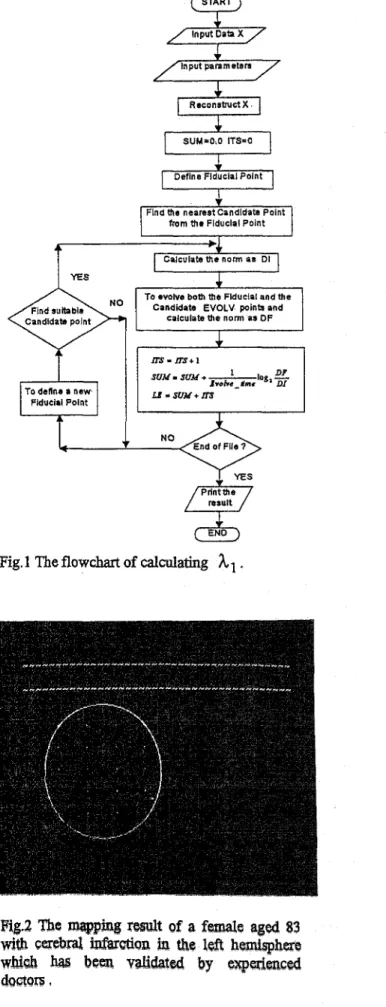
The flowchart of this algorithm is :shown in fig.1. Essentially

this

algorithm itemtively computes the vector distance L of two nearby points and

evolves

its length for a certain propagation time. After m propagation steps we aimate the first positive Lyapunov exponent as:

The source code is written in

FORTRAN

and needs

some

parameters which are iiefined below :

SCAW==noise levelel.0 pv

SCAM=lO% maximum distance

EVOLV=search step for each rqplacement~50

D M - embedding dimension =10

TAU = delay time = the first zero-crossing of autocorrelation function

(2)

The program is compiled with the FORTRAN-

77 compiler and is excuted by a SunStation for its

high speed. Then a 4NN algorithm is used for

interyolation in a 486PC with a color monitor. This is a liiear algorithm easy to understand as the interpolated values merely follow the trend set by the bounding four real electrode values

.

RESULTS

Fig.2 shows one of our results. This is a case of a female aged 83 with cerebral infarction in the left hemisphere. It is evident in this mapping the level of dynamics in the left hemisphere,i.e.the hemisphere with disease,is lower than hat in the right,i.e.the healthy hemisphere.

Such

a result

agrees with the diagnosis of the clinical doctors and also agrees with what have been reported by Goldberger et al. that chaos reveals health[3].

CONCLUSTON

The topographic mapping of EEG using the first positive Lyapunov exponent cau support another view in

brain

function or in clinical decision. Yet a debate about this algorithm is that it is difficult to get the exact dimension for the

sake of data length and the assignment of parameters. One strategy of assigning parameters is to vary one parameter while the others remain

fixed. A suitable value of that parameter is derived if the exponent is bounded in a small range. Besides

,

a 4NN linear interpolation method is rough compared with a curve-fitting

nonlinear algorithm

.

It would have a better performance by a

nonlinear

interpolation.

In our experience, it is valuable of compariug

the mapping on corresponding position of oppo- site side in clinical applications. And the exponent values at Fpl and Fp2 would be smaller if the subjects had the unconscious eyes moving during recording EEG.

This method can complement the techniques of functional image such as MRI and PET to get a deeper understand in brain function.

REFERENCE

[ 11Peter K. H. Wong Introduction to brain

toPo=

graphy , Plenum Press, New

York

aad

Lt91&698,

1991

[21A Wolf ,J. B. Swift,

H,

L,

Swkmq

ami

a.

A, Vastano

,

''Detczrdniq Lyqwov ezponC;et

from a time series" , Physica

E D

,

pp285-3 17

1985

B1A.

L.

Gddbergt3r II,

D,

Rimay and B,

J,

Wa,"

chaos and

" SFbatKi~

Amesican

262, pp.4247

1990

s

3s

h u "

pBy8iQlagy

ReconstructX. I SUM=O;O ITS-0

Define Fiducial Point

i

Find the nearest Candidate Point

from the Fiduclal Point

Calculate the n o m as Dl

To evolve both the FlducIal and the Candidate EVOLV point8 and

calculate the norm as CIF Candidate point

result