An empirical analysis of the real estate market at Taiwan

全文

(1)An empirical analysis of the real estate market at Taiwan By Ching Chun Wei(魏清圳) Assistant Professor, Department of Finance, Providence University, 200 Chungchi Rd., Shalu, Taichung Hsien, 433Taiwan e-mail:ccw@pu.edu.tw Phone: 0918112065 1.Introduction: At 2000, Taiwan by reducing the halve land incremental tax rate and the house tax rate try to stimulate the growing of the real estate market. Beside that, for the expansionary monetary policy, the lower and close to zero interest rate policy adopt to recovery the depression real estate market. However, did these policies exist any significant impact effect to the real estate market? That is did the government policy work or not? This is the main question for our analysis at this paper. This paper attempts to measure and interpret the dynamic effects of government policy and capital market index and other macroeconomic variables shock on the aggregate market for real estate market. The objective of this paper is to examine whether any impact dynamic effects exists between government policies (as well as on capital market, macroeconomic variable index) to the real estate market. By the way, we also try to find out what are the import influence factors to the dynamic real estate market. Lastrapes (2002) used the monthly data, found out that money shocks have real effects on the housing market: both real housing prices and housing sales rises in the short-run in response to positive shocks to the money supply. Wu and Change (2002) used the GDP, M1b, and CPI as macroeconomic indicators, while primary loan interest rate, Taiwan composite stock weight index and non-performing loan ratio as financial indicated then tested the causality between the real estate market and macroeconomic variables and stock market during the financial crisis period in 1992. Their empirical evidences support that Asian crisis did not have a significant impact on the real estate market. From the results of the granger causality test, macroeconomic variables cause real estate variables. Beside that, real estate market and stock market had mutual causalities in past decade. Kim and Lee (2000) analyzed the trends and fluctuations of real estate prices in Korea and offer prices forecasts for the short-and medium run. Empirical results suggested that long-run relationship exists between land price and GDP and between land price and stock prices. Chen and Kanak (1998) examined the dynamic causal relationship between house price and its five determinants, including total house hold income, short run interest rate, stock price index, construction costs, and housing completions, in Taipei new dwelling market. Empirical findings exerts that there is a long-run equilibrium relationship between house price and construction costs, interest rates, total household permanent income, housing completing and stock price index. Darrat and Glascock (1993) used a VAR process to find the relationship of real estate and financial variables. Empirical results suggested that a significant lagged relationship between real estate returns and fiscal policy moves. 1 第五屆全國實證經濟學論文研討會 The 5th Annual Conference of Taiwan's Economic Empirics.

(2) Johnson and Jensen (1999 ) examined the performance of the real estate return, S&P 500 stock return and T-bill return associate with Federal Reserve monetary policy. Empirical evidence suggests that monetary policy has a very broad influence on return to various asset classes. At our paper, we used the Vector Auto-Regressive (VAR) method to find out that the dynamic effect of the government fiscal and monetary policy how to affect the real estate market variables at Taiwan. That is the aim of this paper to analyze real estate market dynamic and causality, which is achieved by the application of VAR model suggested by Sims (1980). Beside that, we extend our analysis by considering the period of the government announcement the reduction of land incremental tax at April 2000, the Asian financial crisis from 1997 to 1998, and the big 921 earthquake at 1999. Here, we use the dummy variables to be the proxy of those periods. The reason for including in this paper is that we want to look such events is there any significant dynamic impact effect to the real estate market at Taiwan. 2.Data Description: The data used in this study are obtained from the Taiwan Economic Data Bank. The total data values commence in 1987/1 and end in 2002/11. Our model comprises several key macroeconomic policy, and financial variables in our empirical study. Here, the amount of the land and building transaction (lndtr,dbtr) are used as proxy variables for the real estate market. However, money supply (dmo) and interest rates (dint) are used as monetary policy indicators, while, tax in land or building (latex, tax) are used as fiscal policy indicators. The building production index (dpr), Taiwan composite stock weight index(taind),and construction index (dbind) are used as financial indicators. Finally, the real estate investments (dinv), business cycle signals (sig), the amount of Taiwanese invest to the Mainland China (chinv) are used as capital flow indicators. 3.Methodology 3.1 ADF test Certain properties of the variables in the model must be checked in order to determine the appropriate specification for estimation purpose. First, it is necessary to determine whether the variables are stationary or non-stationary. Then, this is done by testing the null hypothesis for that each variable included in the model contains a unit root. If the variables are difference stationary, it is appropriate to estimate the GARCH mode by using the first difference of the variables. The unit root test involves testing whether the coefficient of the least square estimate, β ∆ Y =+α t. 0. α +β 1t. 1. in 1. Y + ∑ β Y , is equal to unity. The unit roots are tested by using the Augmented t −1. i. t −i. 2 第五屆全國實證經濟學論文研討會 The 5th Annual Conference of Taiwan's Economic Empirics.

(3) Dickey-Fuller (ADF) test, and the results are reported in table 1. The results of the ADF tests suggest that all the variables are difference stationary. 3.2 Causality test A study of linear causality results can reveal how some interpretations of the real estate index return and fiscal variables and financial variables relationship are formed and how they are affected by a number of macroeconomic events. To illustrate, one can consider two stationary series {Xt} and {Yt} of length n, and estimate the following system of equations:. X Y. t. t. = A(L) X + B ( L )Y t. t −1. + εx , t ………………(1). = C(L) X + D( L)Y + εy , t ………………(2) t t −1. Where A(L),B(L),C(L) and D(L) are all lag polynomials with roots outside the unit circle. The regression error terms, εx,t and εy,t are also assumed to be mutually independent and individual process. The test presented in this paper for whether Y strictly granger causes X involves a standard joint F-test on whether lagged coefficients of Y have significant linear predictive power on X. The null hypothesis is that of no linear causality, implying in equation (1) the coefficient of B(L) are not jointly significant different from zero. Similarly, in the case of testing whether X cause Y, the test will conducted on the coefficients contained in the lag polynomial C(L) to see whether they are jointly significantly different from zero. If both B(L) and C(L) joint tests for significance show they are different from zero, the series are bi-causality related. 3.3.Vector Autoregressive Analysis (VAR): In order to provide further insight into the relationships of the amount of land and building transaction and its determinants, the variance decomposition and impulse response function of the VAR process is introduced at our analysis. The basic description of the VAR process can be found in Littkepohl (1990), Blanchard (1989), Blanchard and Quay (1989), and Sims (1980,1986). Using the VAR methodology, the direct effect of innovations on the dependent variables of the system can be examined. In VAR analysis, the structural model can be written as:. α t Χ t = β ( L) Χ t (−1) + ε t .............(3) Where Χ t. is the vector of dependent variables at time t , α. time t , β (L) is matrix polynomial in the lag operator and disturbances at time t. Here, the matrix. ε. t. is the contemporaneous coefficient matrix at t is the vector of innovations to the structural. captures interaction between the endogenous variables. Equation. (1) can be solvedαby pre-multiplying both sides by α. −1 t. t. , to thus yield the reduced form associated with the. 3 第五屆全國實證經濟學論文研討會 The 5th Annual Conference of Taiwan's Economic Empirics.

(4) structural model: Χ t = α t−1 β ( L) Χ t ( −1) + α t−1ε t .............( 4). or in matrix notation, Χ t = A0 Χ t (−1) + u t .............(5). where. −1 A0 = α t−1 β ( L) , and u t = α ε t. Equation (3) is assumed to be stationary and have a moving average (MA) representation, i.e., Χ t = ∑ A0 u t −i .............(6). where A 0 = I k. is a (KxK) identity matrix. Equation (6) suggests that Χ t. is a linear combination of current and past one-task-ahead forecast errors, u . However, the elements t of Ai. are interpreted as impulse response of the VAR system and trace out the dynamic response of. certain variables to innovations in other variables.. The reduced form model can be estimated by ordinary least squares which yields consistent parameters of. A 0 and. A 1 . The VAR analysis does not impose any restrictions on structural. relationships among variables. Rather, identification of the model is achieved through restrictions on the contemporaneous relations and the variance covariance matrix. This methodology works well in deriving robust estimates of the dynamic relationships between policy variables such as monetary variables and fiscal variables. Since, the main concern is to determine the way in which one country policy affects real estate finance variables, impulse response and variance decomposition techniques are utilized to determine the time path of real estate financial variables responses to monetary policy and fiscal policy shocks among the Taiwan real estate market. 4. Empirical results: 4.1 ADF test: The empirical tools used in this study included the Augmented Dickey-Fuller test (ADF), Granger causality test, impulse response function, variance decomposition based on the vector auto-regressive model are utilized. The ADF test is used to verify the stationary of the time series data. The Granger causality test 4 第五屆全國實證經濟學論文研討會 The 5th Annual Conference of Taiwan's Economic Empirics.

(5) is employed to find the causality relationship between variables. Data is tested for unit roots using the ADF test. The ADF test is used to verify the stationary of the time series data. The results are given in table 1 and 2. The ADF results provide evidence that prevents rejection of the null hypothesis of non-stationary at the 10% level. However, the number of lag lengths, chosen by the minization of AIC is reported at table 3. 4.2 Granger Causality Tests: This section is concerned with test of Granger causality between real estate market and its determinants. The estimated F-statistics of the causality test are reported in table 4 and 5. Row 1 gives the direction of causality, that is, dmo—dbtr denotes that the null hypotheses test is the M1b Granger cause the transaction amount of house transfer. Row 2 and Column 2 show the F-statistics for the null hypotheses of no causality. From the result of F-tests at table 4 and 5, suggest that dmo and chinv Granger cause the transaction amount of house transfer. Then, dmo and dint and sig Granger cause the transaction amount of land transfer. The hypothesis of non-Granger causality is rejected at the 10% level of significant. 4.3 Variance Decomposition: The variance decomposition measure the percentage of variation in real estate market induced by shocks originating from its relevant determinates. The estimates of variance decomposition are shown in table 6 and 7 for a 20 month time horizon. The estimates of variance decomposition include DTAX is shown at table * for 20 months time horizon. The results indicate that the disturbance originating from the amount of land transaction itself contributes up to 76 percent variability two months ahead, approximately 62 percent 4 months ahead. The proportion of variance remains high at 43 percent even until 20 months. Empirical result show that there amount of land transaction estimate an average of 62 percent variability, there remains 38 percent of the variability which is explained by other factors at fourth months. The largest source of the amount of land transaction variance appears to be from DMO, which accounts for approximately 12 percent of the total variance of the amount of land transaction. A relatively high proportion of the amount of land transaction variance induced by monetary variable confirms its importance to dynamic behavior of the amount of land transaction. The second largest source of the amount of land transaction variance appears to be TAIND, which accounts for approximately 8-12 percent of the total variance of the amount of land transaction. At table 6 has been indicated that TAIND as being one of the important factors to the amount of land transaction. Next, table 6 show the results for did not include the D921, DC and DTAX. The results indicate that the disturbance originating from the amount of land transaction itself contributes up to 85% variability two months ahead. Then, the proportion of the variance is at 50 % even until 20 months. The largest source of the amount o f land transaction variance appears to be DMO which accounts for approximately 13% of the total variance of the amount of land transaction. Now, from the table *, the estimation results for us including the D921, DTAX and DC display that the results of variance decomposition for that the amount of land transaction itself contributes up to 66% 5 第五屆全國實證經濟學論文研討會 The 5th Annual Conference of Taiwan's Economic Empirics.

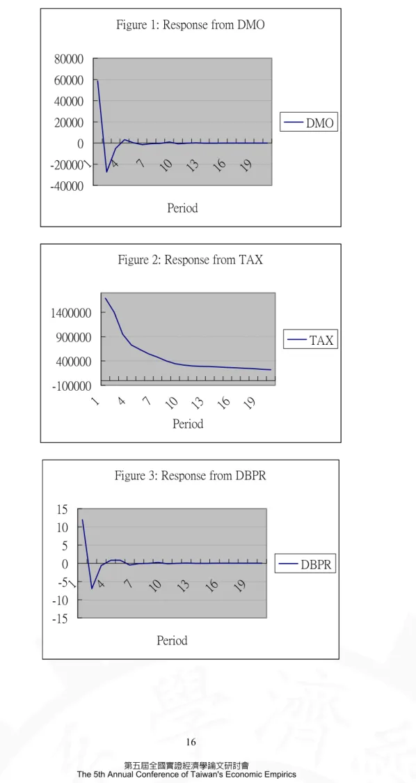
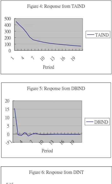
(6) variability at two months ahead. The largest source of the amount of land transaction variance appears to be DMO up to 20% four months but to be Latax 29% at 20 months. The second largest source of the amount of the land transaction appears to be TAIND and DINT that accounts of approximately 7-15% between 4 months and 20 months. Table 6 show the estimation results for including D921. The empirical results of variance decomposition show that the amount of land transaction itself contributes up to 81% variability at two months ahead. The largest source of the amount of land transaction variance appears to DMO up to 12% at twelve months. Finally, the variance decomposition of land transaction for including DC is exhibit at table 6. Results show that amount of land transaction itself contributes up to 80% at two months ahead. The largest source of the land transaction variance appears to be DMO up to 16% at sixteen months. The second largest source of the amount of the land transaction appears to be SIG up to 9% at 20 months. Now, let us turn to the estimation of the variance decomposition for amount of building transaction that includes the D921, DC, and DTAX. From table *, the estimation result tell us that amount of building transaction itself contributes of the 63% at two-month ahead. The importance source of the amount of building transaction variance appears to be DMO, TAX, TAIND approximately 11% at 20 months. However, if we didn’t think about the D921, DC and DTAX, the estimation amount of building transaction itself contributes of the 63% at two months and 15% at twenty months. The important source of the amount of building transaction variance appears to be DMO (14%), DBPR (12%), TAIND (16%),CHINV (10%) and SIG (9%) at 20 months long. Next, the estimation results for including DTAX, DC, and D921 at table 7. Results show that amount of building transaction itself contributes up to 50%, and 67% at two months ahead. The most important source of the amount of building transaction appears to DMO (11%, 16% and 22%), DBPR (20%,13%), TAIND(14% and 11%) and TAX( 10%,14% and 10%) at 20 months. 4.4 Impulse Response function: The variance decomposition estimate the proportion of real estate market variance accounted its determinants. However, it cannot identify whether the impact is positive or negative, or whether it is temporary jump or long-run dynamic persistence. Then, the impulse response function can give an indication of systems dynamic behavior. The impulse response function exhibit that how a variable in the system responds to a single one percent exogenous change in another variable of interest. Figure 1 to figure 11 indicated that the estimated impulse response functions for the amount of building transaction for twenty months. At figure 1, in response to a one standard deviation disturbance in the amount of building transaction, the DMO increase sharply in the first period, then decay very quickly. It implies that the DMO changes have a greater influence on the amount of building transaction at the next period rather than over long-term horizon. Figure 2 show the one standard deviation disturbance originating from TAX, the decrease speed of the TAX is slowly and it sharp declines after the third months. A one standard deviation disturbance originating from DBPR at figure 3 results in a negative impact on the amount of building transaction at first third months and has a large positive impact in fourth months. A one standard deviation disturbance originating from TAIND at figure 4 results in a increase at first months, then the speed adjustment slowly and decrease. 6 第五屆全國實證經濟學論文研討會 The 5th Annual Conference of Taiwan's Economic Empirics.

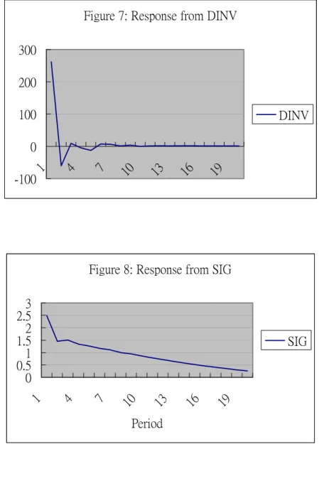
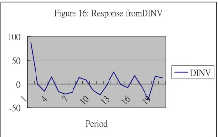
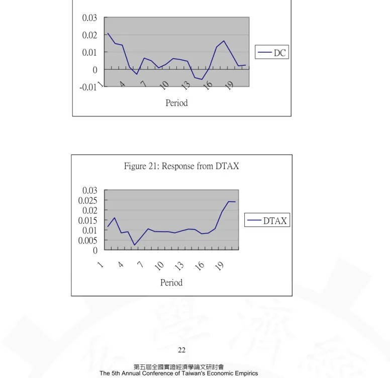
(7) From figure 5, the DBIND has a positive effect on the amount of building transaction. Its greatest positive effect occurs in the first month. At figure 6, the DINT has the greatest positive impact on the amount of building transaction, then decrease after first month and increase at third month, and slowly decrease after three month then close to zero. From figure 7, a one standard deviation disturbance originating from DINV results in an increase, then it decrease and slowly adjustment around the zero. Figure 8 and 9 show the response from SIG and CHINV, the positive increase also exhibit at figure 10 and 11 for the response from D921 and DC. Figure 12 to 21 exhibits the estimated impulse response for the amount of land transaction for 20 months. Figure 12 is the one standard deviation disturbance originating from DMO significantly increase impact in the amount of land transaction, the speed of adjustment is rapidly at first month then decline to negative. Figure 13 is the response from LATAX, we found that significantly increase in the amount of land transaction during the first month, then decline up to five months. However, it sharply increase after 13 months to 20 months. At figure 14, a one standard deviation disturbance originating from TAIND. It initially has a positive impact then sharply decline to zero after one month and close to zero. In figure 15 is the response from DINT. The impulse response results appear suggest that the response around the zero in the amount of land transaction during the first seven month and there is a negative response at 8 to 11 months, then increase at 11 to 12 month, after that sharply decrease to negative. Figure 16 is the response from DINV. The response of DINV has a significantly positive relationship mostly in the first month. But the positive and negative sign are changeable after first month around the zero. Figure 18 is the response from CHINV, it has a positive and significant impact effect of the amount of land transaction at first month, and then it decline after first month, and changeable over the period. As can be seen in the figure 17, 19, 20 and 21 are the response from SIG, D921, DC and DTAX to the amount of land transaction. Those responses are small and positive impact at first month then after that the response are decrease and around the zero.. 5. Conclusion The objective of this paper is to find out the sources and the extent of the amount of the land and building transaction and examine the causality relationship between the amount of land and building transaction and to the other macroeconomic variables. The empirical methodology employed in the ADF tests, Granger Causality tests and the estimation of the variance decomposition and impulse response function. Our findings indicate that the monetary variables (money supply and interest rate) are cause the amount of land transaction but no feedback effects are observed from them. Beside that, the results of the amount of building transaction of causality test show that monetary variables and china investment granger cause the amount of building transaction. In order to test the source of volatility and identify the responses from amount of the land (building) transaction determinants, we decompose the land and building transaction variance. The results indicate that a disturbance originating from money supply and tax accounts the greatest variability to the building and land transaction. From the results of the impulse response function, monetary variables (money supply) and fiscal variable (tax) has a significantly positive relationship in the first periods. Surprising, 7 第五屆全國實證經濟學論文研討會 The 5th Annual Conference of Taiwan's Economic Empirics.

(8) the investment to china also has a significant relationship between them. Generally, from the results of the granger causality tests, variance decomposition, and the impulse response for the variables in this study, show that monetary variables and fiscal variable (tax) are the very important source and relationship to affect the amount of land and building transaction. From our empirical results, we can see that the government’s expansionary monetary policy (lower interest rate) and expansionary fiscal policy(land incremental tax reduction) will be really increase the amount of land and building transaction and improve the benefits to the real estate market in Taiwan now. Reference: Blanchard, O.J., and Quah, D.”The Dynamic Effects of Aggregate Demand and Supply Disturbances”, American Economic Review, Vol. 79, 1989,PP.655-73. Chen, Ming-Chi, and Patel, Knak. “House Price Dynamics and Granger Causality: An Analysis of Taipei New Dwelling Market”, Journal of the Asian Estate Society, Vol. 1, No.1,1998, PP.101-26. Darret,Alif., and John L. Glascock, “Real Estate Returns, Monetary and Fiscal Deficits: Is the Real Estate Market Efficient?”, Journal of the Real Estate Finance and Economics, Vol.2, No.3,1989, PP.197-208. Dickey, D.A. and Fuller, W.A., ”Distribution of Estimator for Auto-regressive Time-Series with a Unit Root”, Journal of the American Statistical Association, Vol.74,1979,PP.427-431. Engle,R.F. and Granger,C.W.J., ”Cointegration and Error and Correction: Representation, Estimation and Testing”, Econometrica, Vol.55,No.2,1987,PP.251-276. Johnson, R.R. and Jensen G.R., ”Federal Reserve Monetary Policy and Real Estate Investment Trust Returns”, Real Estate Finance, Vol. 16, No.1, 1999,PP.52-59. Kim,Kyung-Hwan and Lee, Hahn Shik,”Real Estate Price bubble and Price Forecasts in Korea”, Working Paper, Department of Economics,2000, Sogange University, Korea. Lastrapes, William D.,”The Real Price of Housing and Money Supply Shocks: Time Series Evidence and Theoretical Simulations”, Working Paper, Department of Economics, Terry College of Business, Athens, Georgia. Liitkepohl, H., ”Asymptotic Distribution of Impulse Response Functions and Forecast Error Variance Decomposition of Vector Autoregressive Models”, The Review of Economics and Statistics, 1990, PP.116-125. Sims, C.A. “Macroeconomics and Reality”, Econometrica, Vol.48,1980,PP.1-48. _________”Are Forecasting Model usable for Policy Analysis?”, Federal Reserve Bank of Minneapolis Quarterly Review, 1986,PP.2-16. Wu, Wen-Chieh and Change, Chin-Oh,”Taiwan Real Estate Market in the Post Asian Financial Crisis Period”, Joint Annual Conference of Asian Real Estate Society and American Real Estate and Urban Economics Association, 2002,Seoul,Korea.. 8 第五屆全國實證經濟學論文研討會 The 5th Annual Conference of Taiwan's Economic Empirics.

(9) Table 1:ADF test for Stationary (amount of the Land transaction) Variables. Levels. First Difference. Indtr. -3.77095*. mo. -2.571195. latax. -3.552508*. taind. -3.274742*. int. -0.549492. -5.202529*. inv. -0.980885. -6.396047*. sig. -3.421872**. chinv. -4.138579*. DC. 3.195227*. DTAX. -6.049793*. D921. -5.949790*. -8.837385*. ** indicated significant at least at 5% level, * indicated significant at least at 10% level. Table2:ADF test for Stationary (amount of the building transaction) Variables. Level. First Difference. BTR. -1.624032. -8.272354*. MO. -1.257119. -8.837385*. TAX. -3.552508*. BPR. -1.573629. TAIND. -3.274742**. BIND. -2.013658. -5.485415*. INT. -0.549492. -5.202529*. INV. -0.980885. -6.396047*. SIG. -3.421872*. CHINV. -4.138579*. DC. 3.195227*. DTAX. -6.049793*. D921. -5.949790*. -11.07542*. ** indicated significant at least at 5% level, * indicated significant at least at 10% level. 9 第五屆全國實證經濟學論文研討會 The 5th Annual Conference of Taiwan's Economic Empirics.

(10) Table3: The Selection of Lag Length Lag. AIC. 1. 18.57308. 2. 18.61935. 3. 18.70980. 4. 18.77188. 5. 18.80880. 6. 18.81963. 7. 18.90185. 8. 18.91253. 9. 18.91718. 10. 18.14759. ** indicated significant at least at 5% level, * indicated significant at least at 10% level. Table4: F-statistics for tests for Granger Causality F-value. p-value. DMO→SNDTR. 7.20827. 0.00097*. LNDTR→DMO. 1.13147. 0.32484. LATAX→LNDTR. 1.75264. 0.17641. LNDTR→LATAX. 2.00429. 0.13791. TAIND→LNDTR. 0.28152. 0.75897. LNDTR→TAIND. 0.31768. 0.72824. DINT→LNDTR. 2.63356. 0.07549*. LNDTR→DINT. 0.8877. 0.41339. DINV→LNDTR. 2.07389. 0.12871. LNDTR→DINV. 1.48065. 0.23026. SIG→LNDTR. 4.68802. 0.01035*. LNDTR→SIG. 1.87815. 0.15584. CHINV→LNDTR. 1.28728. 0.27963. LNDTR→CHINV. 0.00464. 0.99537. *indicated at least significant at 10% level.. 10 第五屆全國實證經濟學論文研討會 The 5th Annual Conference of Taiwan's Economic Empirics.

(11) Table5:F-statistics for Tests of Granger-Causality(amount of building transaction) F-value. p-value. DMO→DBTR. 6.25836. 0.00236*. DBTR→DMO. 1.08242. 0.34097. TAX→DBTR. 0.18142. 0.94778. DBTR→TAX. 1.10617. 0.35546. DBPR→DBTR. 0.66698. 0.51452. DBTR→DBPR. 3.22538. 0.04205*. TAIND→DBTR. 0.2429. 0.78461. DBTR→TAIND. 0.09013. 0.91385. DBIND→DBTR. 0.00318. 0.99683. DBTR→DBIND. 0.75032. 0.47369. DINT→DBTR. 0.22185. 0.80126. DBTR→DINT. 0.10293. 0.90224. DINV→DBTR. 1.28751. 0.2785. DBTR→DINV. 2.78809. 0.06421*. SIG→DBTR. 0.62299. 0.53749. DBTR→SIG. 1.12781. 0.32602. CHINV→DBTR. 3.80847. 0.02478*. DBTR→CHINV. 0.03411. 0.96648. *indicated at least significant at 10% level.. 11 第五屆全國實證經濟學論文研討會 The 5th Annual Conference of Taiwan's Economic Empirics.

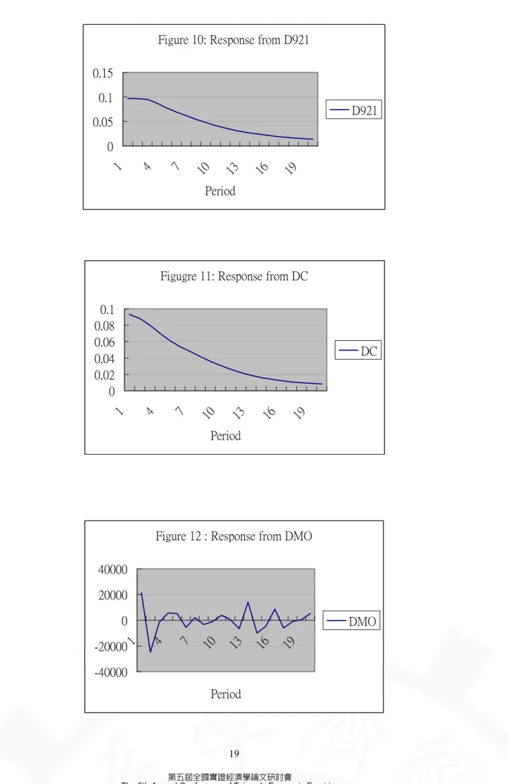
(12) Table6: Variance Decomposition of the amount of land transaction Months LNDTR. DMO. LATAX TAIAD DINT DINV. SIG. CHINV. DTAX. (Include. 2. 76.225. 9.614. 1.092. 0.123. 0.956. 8.08. 0.286. 0.1909. 3.403. DTAX). 3. 70.726. 9.618. 1.393. 2.589. 2.136. 8.126. 1.626. 0.651. 3.136. 4. 62.034. 11.715 1.844. 2.208. 2.377. 9.057. 5.737. 2.054. 2.975. 8. 55.206. 9.515. 2.754. 7.209. 3.805. 7.57. 6.116. 4.364. 3.46. 12. 45.958. 13.27. 2.697. 7.694. 4.634. 6.676. 7.546. 6.916. 4.611. 16. 44.978. 13.049 2.639. 8.793. 4.874. 6.188. 6.657. 7.687. 5.132. 20. 43.082. 12.097 2.701. 12.121. 5.26. 6.211. 6.322. 7.378. 4.829. Months LNDTR. DMO. LATAX TAIAD DIAT DINV. SIG. CHINV. (Include. 2. 84.645. 8.823. 0.583. 2.23E-05. 2.292. 2.562. 0.533. 0.762. D921,DC,. 3. 80.533. 8.433. 0.691. 1.855. 2.164. 2.741. 2.35. 1.234. DTAX). 4. 73.885. 9.916. 1.358. 1.595. 2.89. 3.103. 5.223. 2.03. 8. 64.104. 8.609. 2.9. 5.54. 4.689. 3.417. 6.14. 4.594. 12. 53.828. 13.129 4.141. 6.414. 5. 3.207. 7.882. 6.398. 16. 51.972. 13.601 3.826. 7.047. 5.368. 3.747. 7.281. 7.158. 20. 50.092. 12.707 3.904. 8.667. 6.447. 3.825. 6.881. 7.476. Months. LNDTR. DMO. (Include. 2. 6.703. 15.02. D921,. 3. 59.635. DTAX,. 4. DC). LATAX. 0.056. TAIND. DINT. DINV. SIG. CHINV. D921. DC. DTAX. 0.98. 7.328. 5.785. 3.802. 0.071. 0.3. 0.013. 0.942. 16.494 3.092. 1.109. 8.485. 5.2. 4.122. 0.169. 0.297. 0.416. 0.979. 52.075. 19.953 3.937. 4.557. 7.122. 4.389. 4.522. 0.345. 1.458. 0.612. 1.032. 8. 33.834. 20.799 6.719. 11.973. 11.67. 4.71. 3.761. 1.711. 2.252. 1.438. 1.136. 12. 29.005. 16.469 14.147. 14.699. 11.41. 4.797. 3.717. 1.4. 1.66. 1.637. 1.06. 16. 24.6429. 14.638 23.025. 11.292. 9.071. 4.402. 3.275. 1.795. 3.682. 1.54. 2.637. 20. 23.421. 11.282 29.02. 8.477. 6.719. 3.459. 2.411. 2.744. 5.071. 2.832. 4.565. 12 第五屆全國實證經濟學論文研討會 The 5th Annual Conference of Taiwan's Economic Empirics.

(13) Months LNDTR. DMO. LATAX TAIND DINT DINV. SIG. CHINV. D921. (Include. 2. 81.528. 8.538. 0.279. 0.002. 5.279. 3.022. 0.573. 0.486. 0.293. D921). 3. 77.847. 8.315. 0.568. 2.531. 5.076. 3.045. 1.361. 0.723. 0.534. 4. 72.465. 10.605 1.082. 2.185. 5.637. 3.006. 3.357. 1.186. 0.476. 8. 62.308. 9.249. 2.436. 6.007. 0.66. 3.899. 4.299. 4.663. 0.479. 12. 52.16. 12.085 4.107. 6.412. 7.114. 4.1. 6.237. 6.146. 1.643. 16. 51.435. 12.742 3.94. 6.89. 6.429. 4.163. 5.587. 6.662. 2.154. 20. 49.608. 11.813 4.053. 8.116. 6.87. 4.804. 5.451. 7.022. 2.263. Months LNDTR. DMO. LATAX TAIND DINT DINV. SIG. CHINV. DC. (Include. 2. 79.955. 10.643 0.0011. 0.861. 1.432. 3.988. 1.061. 1.007. 1.053. DC). 3. 73.497. 9.718. 2.771. 1.589. 3.641. 4.904. 0.971. 2.669. 4. 65.48. 11.274 1.242. 2.324. 4.418. 3.304. 6.031. 1.758. 4.189. 8. 55.329. 11.211 2.232. 4.859. 4.525. 3.562. 7.144. 4.758. 6.399. 12. 44.726. 15.45. 4.777. 5.299. 5.614. 3.227. 9.321. 4.935. 6.65. 16. 45.043. 16.416 4.568. 5.579. 5.045. 3.224. 9.225. 4.857. 6.043. 20. 45.583. 15.469 4.455. 5.812. 5.051. 3.318. 9.092. 5.073. 6.147. 0.24. 13 第五屆全國實證經濟學論文研討會 The 5th Annual Conference of Taiwan's Economic Empirics.

(14) Months. DBTR. DMO. 2. 63.245. 9.29. 3. 48.923. 4. TAX. DBPR. TAIND. DIAT. DINV. SIG. CHZIV. D921. DC. 4.343. 1.058. 7.255. 0.083. 4.632. 0.192. 4.372. 2.859. 0.235. 0.231. 9.389. 7.42. 0.785. 11.36. 0.158. 3.435. 1.491. 7.084. 2.151. 0.592. 0.252. 45.476. 8.511. 8.088. 0.929. 11.594. 0.201. 3.198. 1.589. 6.398. 2.121. 0.757. 0.302. 8. 37.12. 7.032. 14.12. 1.815. 11.447. 1.028. 4.772. 2.857. 7.176. 2.042. 0.877. 0.79. 12. 33.28. 7.768. 12.1. 3.199. 13.503. 1.173. 4.625. 4.344. 6.379. 2.055. 1.54. 1.327. 16. 29.468. 10.649. 12.24. 3.964. 11.799. 1.048. 5.374. 6.225. 5.646. 2.391. 1.755. 2.041. 20. 26.763. 11.878. 11.26. 4.524. 11.311. 1.479. 5.94. 7.249. 5.912. 2.661. 2.222. 1.811. Months. DBTR. DMO. TAX. DBPR. TAIND. DBIND. DINT. DINV. CNINV. 2. 62.728. 19.795. 0.107. 5.246. 1.222. 0.054. 4.2. 1.74. 2.8. 2.108. 3. 40.713. 17.698. 0.234. 7.121. 1.068. 10.922. 2.674. 1.108. 16.458. 2.002. 4. 37.129. 16.446. 1.816. 6.178. 3.066. 10.865. 5.459. 1.185. 15.958. 1.897. 8. 27.376. 15.511. 6.245. 9.086. 13.086. 7.337. 3.67. 2.908. 12.056. 2.725. 12. 19.913. 13.006. 7.899. 9.878. 16.77. 6.05. 4.009. 4.403. 11.861. 6.206. 16. 16.89. 16.157. 7.117. 9.563. 16.325. 6.044. 3.73. 7.059. 8.994. 8.119. 20. 14.909. 14.324. 7.114. 11.68. 15.774. 6.274. 3.442. 6.475. 10.875. 9.135. Months. DBTR. DMO. TAX. DBPR. TAIND. DBIND. DINT. DINV. CNINV. SIG. SIG. DTAX. 2. 50.396. 11.988. 1.893. 14.63. 0.897. 0.0004. 9.638. 1.849. 7.245. 0.199. 1.264. 3. 32.01. 6.822. 0.981. 20.99. 0.895. 2.053. 17.75. 0.989. 14.521. 0.372. 2.623. 4. 28.462. 5.997. 1.657. 20.74. 3.581. 2.219. 17.17. 0.886. 14.25. 1.514. 3.527. 8. 20.321. 4.014. 6.038. 20.29. 13.861. 2.298. 14.46. 3.167. 11.488. 1.115. 2.953. 12. 18.024. 4.847. 10.21. 20.22. 14.722. 2.961. 12.08. 2.947. 8.443. 2.413. 3.133. 16. 12.863. 13.497. 10.43. 14.89. 16.563. 4.482. 11.58. 3.619. 5.948. 3.546. 2.58. 20. 11.531. 11.842. 10.7. 20.38. 14.464. 4.196. 10.5. 33.36. 5.755. 5.004. 2.273. 14 第五屆全國實證經濟學論文研討會 The 5th Annual Conference of Taiwan's Economic Empirics. DTAX.

(15) Months. DBTR. DMO. 2. 50.175. 1.779. 3. 22.229. 4. TAX. DBPR. TAIND. DBIND. DINT. DINV. CNINV. 0.191. 15.13. 1.444. 11.412. 7.5. 1.761. 5.063. 5.524. 0.019. 5.617. 7.431. 19.99. 6.221. 21.958. 4.36. 0.782. 4.506. 6.906. 0.01. 20.031. 7.631. 6.702. 20.19. 5.649. 20.538. 6.83. 0.705. 4.612. 7.098. 0.016. 8. 16.592. 7.819. 9.071. 23.16. 9.099. 12.215. 6.58. 7.933. 2.831. 4.692. 0.023. 12. 9.437. 13.954. 15.08. 12.89. 16.467. 8.155. 4.14. 11.72. 2.071. 6.036. 0.059. 16. 12.233. 17.186. 14.77. 13.05. 15.663. 6.818. 4.32. 9.672. 1.622. 4.683. 0.043. 20. 12.125. 15.88. 14.75. 13.15. 14.634. 7.719. 4.11. 10.22. 1.893. 5.474. 0.044. Months. DBTR. DMO. TAX. DBPR. TAIND. DBIND. DINT. DINV. CNINV. 2. 67.062. 16.398. 2.008. 6.036. 4.999. 0.0004. 0.68. 1.216. 2.624. 4.133. 0.038. 3. 47.727. 15.171. 5.166. 11.05. 6.731. 5.488. 0.657. 1.785. 3.099. 3.965. 0.05. 4. 43.555. 19.915. 5.061. 10.35. 6.482. 5.01. 0.686. 2.519. 2.702. 3.621. 0.066. 8. 30.867. 22.686. 8.778. 7.943. 11.5. 3.978. 2.763. 4.09. 2.072. 4.484. 0.156. 12. 22.78. 22.835. 8.805. 7.698. 8.905. 5.638. 1.779. 5.478. 3.874. 11.85. 0.403. 16. 18.463. 24.596. 11.07. 6.425. 10.666. 4.838. 2.838. 6.63. 3.721. 9.842. 0.409. 20. 17.423. 22.679. 10.67. 7.256. 11.489. 5.038. 4.381. 6.343. 4.205. 10.13. 0.385. 15 第五屆全國實證經濟學論文研討會 The 5th Annual Conference of Taiwan's Economic Empirics. SIG. SIG. DTAX. D921.

(16) Figure 1: Response from DMO 80000 60000 40000 20000. DMO. 19. 16. 13. 10. 4. 1. -20000. 7. 0 -40000 Period. Figure 2: Response from TAX. 1400000 900000. TAX. 400000. 19. 16. 13. 10. 7. 4. 1. -100000 Period. Figure 3: Response from DBPR. 19. 16. 13. 10. 7. DBPR 4. 1. 15 10 5 0 -5 -10 -15. Period. 16 第五屆全國實證經濟學論文研討會 The 5th Annual Conference of Taiwan's Economic Empirics.

(17) Figure 4: Response from TAIND 500 400 300 200 100 0. 19. 16. 13. 10. 7. 4. 1. TAIND. Period. Figure 5: Response from DBIND 20 15 10. DBIND. 5. 19. 16. 13. 10. 4. 1. -5. 7. 0. Period. Figure 6: Response from DINT 0.15 0.05. 19. 16. 13. 10. 7. 1. -0.05. 4. DINT. -0.15 Period. 17 第五屆全國實證經濟學論文研討會 The 5th Annual Conference of Taiwan's Economic Empirics.

(18) Figure 7: Response from DINV 300 200 100. DINV. 19. 16. 13. -100. 10. 7. 4. 1. 0. Figure 8: Response from SIG 3 2.5 2 1.5 1 0.5 0 19. 16. 13. 10. 7. 4. 1. SIG. Period. Figure 9: Response from CHINV 150000 100000 50000. CHINV. 19. 16. 13. 10. 7. -50000. 4. 1. 0. Period. 18 第五屆全國實證經濟學論文研討會 The 5th Annual Conference of Taiwan's Economic Empirics.

(19) Figure 10: Response from D921 0.15 0.1 D921. 0.05. 19. 16. 13. 10. 7. 4. 1. 0. Period. Figugre 11: Response from DC 0.1 0.08 0.06 0.04 0.02 0. 19. 16. 13. 10. 7. 4. 1. DC. Period. Figure 12 : Response from DMO 40000 20000 0 19. 16. 13. 10. 7. 4. 1. -20000. DMO. -40000 Period. 19 第五屆全國實證經濟學論文研討會 The 5th Annual Conference of Taiwan's Economic Empirics.

(20) Figure 13: Response from LATAX 600000 400000 LATAX 200000. 19. 16. 13. 10. 7. 4. 1. 0. Period. Figure 14: Response from TAIND 200 150 100. TAIND. 50. 19. 16. 13. 10. 4. 1. -50. 7. 0 Period. Figure 15: Response from DINT. 20. 17. 14. 11. 7. 4. DINT. 1. 0.03 0.02 0.01 0 -0.01 -0.02 -0.03. Period. 20 第五屆全國實證經濟學論文研討會 The 5th Annual Conference of Taiwan's Economic Empirics.

(21) Figure 16: Response fromDINV 100 50 DINV. 19. 16. 13. -50. 10. 7. 4. 1. 0. Period. Figure 17: Response from SIG 0.4 0.3 0.2 0.1 0 -0.1 -0.2 -0.3 -0.4 -0.5. 19. 16. 13. 10. 7. 4. 1. SIG. Period. Figure 18: Response from CHINV. 19. 16. 13. 10. 7. CHINV 4. 1. 40000 30000 20000 10000 0 -10000 -20000. Period. 21 第五屆全國實證經濟學論文研討會 The 5th Annual Conference of Taiwan's Economic Empirics.

(22) Figure 19: Response from D921 0.03 0.02 0.01 0 -0.01 -0.02 -0.03 -0.04 -0.05. 19. 16. 13. 10. 7. 4. 1. D921. Period. Figure 20: Response from DC 0.03 0.02 0.01. DC. 19. 16. 13. 10. 7. 1. -0.01. 4. 0. Period. Figure 21: Response from DTAX 0.03 0.025 0.02 0.015 0.01 0.005 0 19. 16. 13. 10. 7. 4. 1. DTAX. Period. 22 第五屆全國實證經濟學論文研討會 The 5th Annual Conference of Taiwan's Economic Empirics.

(23)