動態變更查詢優先權的布隆過濾器

國

立

交

通

大

學

網路工程研究所

碩

士

論

文

動態變更查詢優先權的布隆過濾器

Dynamic Reordering Bloom Filter

研 究 生：張大鈞

指導教授：陳 健 教授

動態變更查詢優先權的布隆過濾器

Dynamic Reordering Bloom Filter

研 究 生：張大鈞 Student：Da-Chung Chang

指導教授：陳 健 Advisor：Chien Chen

國 立 交 通 大 學

網 路 工 程 研 究 所

碩 士 論 文

A Thesis

Submitted to Institute of Network Engineering College of Computer Science

National Chiao Tung University in partial Fulfillment of the Requirements

for the Degree of Master

in

Computer Science October 2013

Hsinchu, Taiwan, Republic of China 中華民國一百零二年十月

動態變更查詢優先權的布隆過濾器

研究生：張大鈞 指導教授：陳 健 國 立 交 通 大 學 網 路 工 程 研 究 所

中文摘要

布隆過濾器是一種節省記憶體空間的資料結構，提供儲存靜態資料集合與集合成員 確認的功能。布隆過濾器被運用於許多的領域，例如在於分散式系統的領域，布隆過濾 器可被用於系統內同儕之間的訊息交換以節省網路頻寛的使用。以共同合作的網頁代理 伺服器而為例，網頁代理伺服器之間會週期性的將目前快取的資料特徵值儲存於布隆過 濾器中並互相交換。當網頁代理伺服器收到一筆查詢資料的請求但並沒有快取相關的資 料時，則可以藉由查詢布隆過濾器得知哪個同儕具有所需要的資料而向其發出資料請求 的封包以避免不必要的封包發送。對於現存的文獻中，於多個布隆過濾器中進行成員確 認的方法都是採用循序搜尋的架構。不幸的，多個布隆過濾器的查詢次序是不可被預測， 若被查詢的資料是儲存於具有較低查詢優先權的布隆過濾器時，就需要較高的查詢成本。 本文針對上述的議題提出了一種能夠節省查詢成本的方法。經由參考時域性的分佈而即 時的更新相關的布隆過濾器之查詢優先權，分配給經常被查詢的布隆過濾器較高的查詢 優先權，藉以減少不必要的布隆過濾器進行成員確認的成本。對於現存的方法而言，本 文所提出的方法至多可以節省 40%的搜尋成本。經由不同應用領域的日誌檔驗證得知， 本文的方法面對不同傾向的時域性分佈都具有較好的表現。 關鍵字：布隆過濾器、動態布隆過濾器、壓縮性資料結構、網頁代理伺服器、時域性

Dynamic Reordering Bloom Filter

Student: Da-Chung Chang Advisor: Dr. Chien Chen

Institute of Network Engineering National Chiao Tung University

Abstract

Bloom Filter is a space-efficient data structure for representing static data set and supporting membership check of the set. Bloom Filter is widely applied to many fields such as distributed systems. Bloom Filter can be used for saving the network bandwidth when interchanging information with peers in a distributed system. For example in cooperative web proxy design, web proxies periodically index their cache data to Bloom Filters and exchange them with each other. A web proxy can check Bloom Filters to find out which proxy cache the web document and send a query directly to that proxy. It can avoid broadcasting requests to all the peers which may not have cached data. To check a membership in multiple set of bloom filters in a dynamic bloom filter, a sequential search order is usually used. Since distribution of web queries usually has temporal locality feature which means there is a very high probability that the recent web query will be queried again in a short future. Therefore to save search cost, we propose a scheme that can dynamically reorder the searching sequence of multiple bloom filters in a dynamic bloom filter. Simulation results show that our scheme on average has 40% better in searching performance comparing with the sequential methods, which is verified via three different trace log files.

keywords: bloom filter; dynamic bloom filter; compact data structure; web proxy; temporal locality

誌謝

本篇論文的完成，我要感謝這些日子給予我協助和鼓勵的人。首先要感謝我的指導 教授 陳健博士，雖然在這段期間研究上常常遇到挫折，但陳老師對我的指導跟教誨， 讓我在遇到困難時找到解決方法，最終得以完成學位論文。在學習如何研究的過程中， 老師也給了許多不同的想法和概念，讓我學習了許多實用的研究方法，在此表達最誠摯 的感謝。同時也感謝我的口試委員，簡榮宏教授、王國禎教授與朱煜煌博士，在口試時 提出了許多寶貴意見，讓我受益良多。 感謝張哲維學長在運用數學模型分析問題的部份給予的指導，讓我可以了解到抽象 的概念如何以數學方程式具體的表達出來。感謝同學蔡世仁與我分享賽斯心法，讓我了 解到自己必須先肯定自己的能力，才能達成自己的夢想。對於論文寫作的部份也特別感 謝黃璟勝博士的協助，讓我更能夠了解英文寫作時相關的技巧與需要注意的部份，使得 文章呈現的內容能夠更加明確。同時也感謝實驗室的學長學弟們，謝謝他們陪我度過充 實的研究生活，在我需要協助時不吝伸出援手幫忙。 最後，我要感謝家人對我的關懷與支持，父母含辛茹苦的栽培，讓我能夠無後顧之 憂的專心於研究所的課程，哥哥也不時的會打電話關心我的研究進度，在此要向他們致 上最高的感謝。

本文目錄

中文摘要 ... ii Abstract ... iii 誌謝 ... iv 本文目錄 ... v 圖目錄 ... vii 表目錄 ... viii Chapter 1 : Introduction ... 1

Chapter 2 : Related Works ... 4

2.1 One Memory Access Bloom Filters ... 4

2.2 The Dynamic Bloom Filter ... 4

2.3 Time-Dependent Bloom Filter ... 5

2.4 Temporal Locality Feature ... 5

Chapter 3 : Dynamic Reordering Bloom Filters... 7

3.1 Motivation ... 7

3.2 Policy of Changing Query Priority ... 7

3.3 Promotion of System Performance ... 8

3.4 Query Index ... 10

Chapter 4 : System Performance Analysis ... 12

4.1 Markov chain analysis ... 12

Chapter 5 : Simulation Results ... 15

5.1 Performance of the Most Popular Block ... 15

5.2 Artificial Data Sets ... 17

5.3 NASA Web Server Trace Log File ... 18

5.4 eDonkey tracker trace log file ... 19

5.6 Changing of False Positive Ratio of Bloom-g Filter ... 21

圖目錄

Figure 1-1 Architecture of Bloom Filter... 1

Figure 2-1 Architecture of Bloom-1 Filter ... 6

Figure 2-2 Architecture of Dynamic Bloom Filter ... 6

Figure 2-3 An example of distribution of temporal locality [18] ... 6

Figure 3-2-1 Query order changing of multiple BFs ... 8

Figure 3-3-1 Competition between multiple BFs ... 9

Figure 3-3-2 Architecture of replacing BFs with OMABFs ... 9

Figure 3-4-1 Architecture of adding Query Index ... 10

Figure 3-4-2 Architecture of Dynamic Reordering Bloom Filter... 11

Figure 4-1 Initial transition probabilities ... 14

Figure 4-2 States and their transition probabilities ... 13

Figure 4-3 Expression of Markov chain ... 14

Figure 4-4 Evaluation of memory access times for a specific Bloom Filter ... 14

Figure 5-1-1 Performance evaluated by simulation and Markov Chain ... 16

Figure 5-2-1 Performance for various α ... 18

Figure 5-3-1 Performance verification using trace log from NASA web server... 19

Figure 5-4-1 The performance of dynamic bloom filters verified by eDonkey tracker log ... 20

表目錄

Table 5-1-1 Experiment parameters ... 15

Table 5-2-1 Parameters for simulation test data ... 17

Table 5-3-1 Profile of NASA web server trace log ... 18

Table 5-4-1 Profile of eDonkey trace log file... 19

Table 5-5-1 Profile of web proxies trace log files ... 20

Table 5-6-1 False Positive Ratio of N-MABF for Different Number of Block ... 21

Chapter 1: Introduction

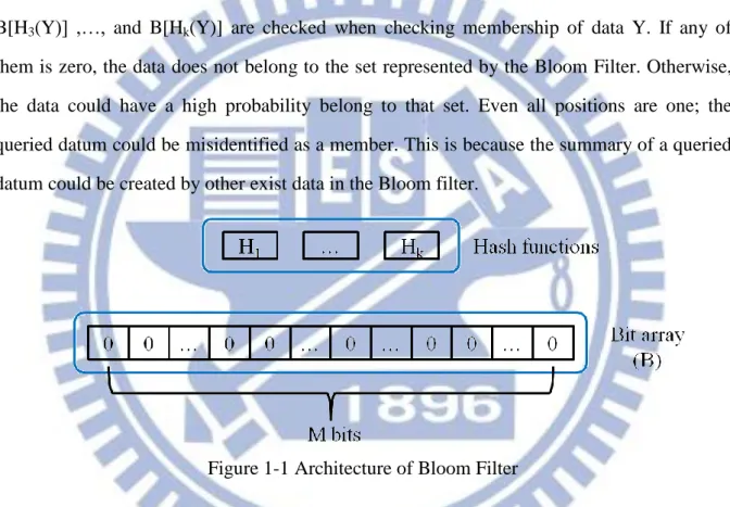
Bloom filters (BF) were proposed by Burton Bloom in 1970 [1] consists of two components: (1) Bit array (B) with m-bits. (2) A group of hash functions (H). Its architecture is shown in Figure 1-1. The k represents the number of H. The B is initialized with zero. Hash function Hi (0 < i ≤ k) maps the data to each of k positions of B for setting B[H1(X)] = 1,

B[H2(X)] = 1,…, and B[Hk(X)] = 1 when inserting data X. Bits of B[H1(Y)] , B[H2(Y)],

B[H3(Y)] ,…, and B[Hk(Y)] are checked when checking membership of data Y. If any of

them is zero, the data does not belong to the set represented by the Bloom Filter. Otherwise, the data could have a high probability belong to that set. Even all positions are one; the queried datum could be misidentified as a member. This is because the summary of a queried datum could be created by other exist data in the Bloom filter.

False positive ratio is used to describe the probability that the data which are not the members of the set are identified as the members. The false positive ratio can be formulated as k m kn

e

fp



(

1



/

)

(1) where variable n is number of elements in the set; and m is memory size. For the specific ratio of m / n, the optimal number of hash functions k can be expressed as

2

ln

n

m

k



(2)

Bloom Filter has the benefit in saving memory space and checking membership in constant time. It helps applications to increase their performance with fewer extra resources consumption. Many variants of Bloom Filter are proposed for applying to different research fields. Counting Bloom Filter [2, 3 and 4] replaces one bit with several bits for measuring number of members set in the same location in the Bloom Filter and for accurately deleting a bit form a particular location. Compressed Bloom Filter [5] is proposed to reduce Bloom Filter size for saving bandwidth when exchanging Bloom Filter between peers. Packet classification [6, 7] uses multiple Bloom Filters to rapidly identify which interface can be used to forward a packet. Hierarchical Bloom Filter [8] helps to deeply inspect the payload of a packet for security issues. LIPSIN [9] inserts routing information of a multicast group into Bloom Filter and replaces the packet header with the Bloom Filter such that it can support large-scale multicast since the number of multicast group is too large to be maintain by the routers on the routing paths. Besides, Bloom Filter is introduced to distribution system such as cooperative web proxy. The proxies set their own cache information to Bloom Filter and exchange them with each other to reduce network traffic consumption. In decades ago, the loading of web server substantially increased with the number of clients. For this reason, the idea of web proxy was proposed by [10] for mitigating network traffic through the Internet. Web proxy locates in the network edge and caches partial content of web servers. Once a client sends a web document request, web proxy sends related document back if the document is cached locally. In order to gain more benefits from web proxy, the idea of cooperative web proxy which applies to Bloom Filter was proposed by [11]. Each proxy stores a caching data summary represented by a group of Bloom Filters. The summary includes a directory of cached web documents in others proxies. When a client request misses in the local cache, web proxy checks the summaries to infer which proxy has the required document. Then the web proxy redirects the request to the corresponding proxy and fetches the document back. Otherwise, the proxy directly sends request to the web server for retrieving the document. To check a membership in multiple bloom filters, a sequential search order is usually used. However, a larger searching cost may be incurred if frequently-required documents are stored in the Bloom Filters which are located in the lower search priority. Since distribution of web

queries usually has temporal locality feature which means there is a very high probability that the recent web query will be queried again in a short future. Therefore to save search cost, we propose a scheme that can dynamically reorder the searching sequence of multiple bloom filters in a dynamic bloom filter.

The remaining sections are organized as follows: Section II summarizes the related articles realted with Bloom Filter. Section III introduces the stucture of our proposaed dynamic reordering bloom fiter. Section IV analyses the performance of our design using Markov Chain. Section V discusses the simulation results from three real trace logs. Section VI gives the conclusion.

Chapter 2: Related Works

2.1 One Memory Access Bloom Filters

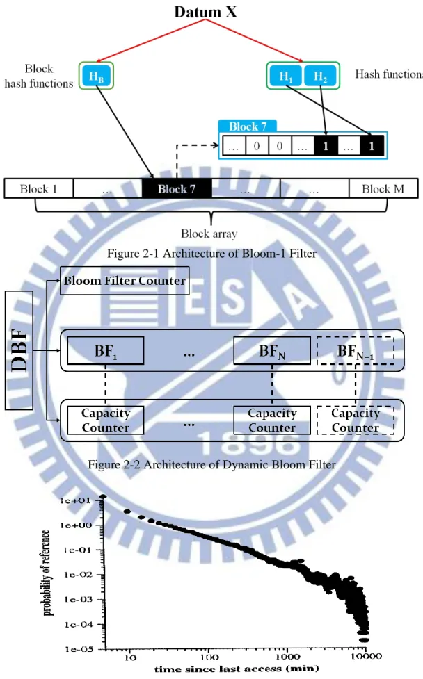
Performance of Bloom Filter is dominated by two factors: (1) memory size (2) the number of hash functions. The growth of memory size is rapider than that of memory access speed. The memory access speed may become a bottleneck when much lower false positive ratio is required by some applications. To achieve lower false positive ratio with slowly increasing memory access times, One Memory Access Bloom Filter (OMABF) is proposed [12]. The basic idea is to replace mapping a datum to k bits randomly selected from the bit array by mapping a datum to k bits in a block. A block is defined as continuous „w‟ bits and can be fetched from memory to the processor in one memory access. Bloom-1 Filter is alias of OMABF. Architecture of Bloom-1 Filter is shown in Figure 2-1. A block array is used for saving data. Block hash function is firstly used to choose a specific block from the block array when accessing a datum. Then, Hash functions are used to set or get the bits to and from the block for the datum.

2.2

The Dynamic Bloom Filter

Applications of dynamic data set are more common than static one in the real world, such as distributed hash table of peer-to-peer, network traffic measurements, etc. Dynamic Bloom Filter (DBF) is therefore proposed [13]. DBF can be applied to manage dynamic data set and distributed systems. It consists of three components: (1) A Bloom Filter Counter for recording the number of Bloom Filters included by DBF (2) Many Bloom Filters for managing dynamic data sets (3) One capacity counter for each Bloom Filter. For applications in a distributed system, one Bloom Filter is mapped to one peer. Once information of any peer needs to be modified, the corresponding Bloom Filter is rebuilt. Sequentially searching Bloom Filters is used to perform membership check in DBF. The searching order starts from number BF1. Architecture of Dynamic Bloom Filter is shown in Figure 2-2. Squares drawn with solider line represent items which already exist in DBF; squares drawn with dash line represent items which will be created if there is no space for saving more data. Bloom Filter

Counter is used to indicate which Bloom Filter is used to store a new datum or is the last one needed to be checked. The capacity counter associates with the Bloom Filter indicated by Bloom Filter Counter is checked when a new datum is needed to be inserted. The datum is inserted into the Bloom Filter if the value of the capacity counter is not zero. Otherwise, Bloom Filter Counter is increased by one. In the same time, new Bloom Filter and corresponding capacity counter are created. The datum is therefore inserted into the new Bloom Filter. The new capacity counter is then decreased by one.

2.3

Time-Dependent Bloom Filter

Time-Dependent Bloom Filter (TMBF) [14] considers the issue of temporal locality. TMBF queries data in the order which is opposite to DBF. Emulation of the literature indicates that TMBF can save up to 20% of extra query cost than DBF.

2.4

Temporal Locality Feature

There are many literatures [15, 16, and 17] accounting for temporal locality appearing in the request stream of web proxy. Temporal locality consists of two distinct phenomena: (1) Long-term: Web document is really popular. (2) Short-term: Massive references of correlations appear in short time interval. Web documents which repeatedly appear such as logo image are the main factor to form the long-term temporal locality. Distribution of long-term temporal locality is similar to Zipf-like one. Short-term temporal locality may be caused by different caching policy between web browser and proxy or by temporal correlation of multiple documents. An example of distribution of temporal locality is shown in Figure 2-3. It shows the probability of a document is queried again as a function of the time since the last access to this document. The probability is lower and lower with elapsed time. The literature [18] found that the probability is roughly proportional to 1/t if the document is queried at time t after it has been last queried. However, the probability rises again in some points in time. It may be caused if a user tends to query recently-read documents again on daily basis.

Figure 2-1 Architecture of Bloom-1 Filter

Figure 2-2 Architecture of Dynamic Bloom Filter

Chapter 3: Dynamic Reordering Bloom Filters

In this section, we introduce how to achieve lower cost for checking and maintaining membership in multiple bloom filters. Two factors are considered: (1) Policy of changing the query order of Bloom Filters (2) Reducing the overhead caused by changing the order. Our scheme improves the effect of search based on TMBF.

3.1

Motivation

Distribution of queried web documents is unpredictable due to the feature of temporal locality. Popularity of the same web document may have significant difference in different time slots. Recent researches for membership check in multiple Bloom Filters uses sequential search because of the lack of relationship between any two data stored in the different Bloom Filters. Cost of membership check is increased substantially if many frequently queried web documents are stored in the Bloom Filters which have lower query order. For mitigating the cost, this thesis proposes a concise scheme to immediately modify the query order of each Bloom Filter by referencing distribution of temporal locality. Higher query orders are assigned to the Bloom Filters which include frequently queried web documents. These Bloom Filters are called Popular Bloom Filters in later paragraph. Similarly, Bloom Filters which mostly include infrequently queried web documents gain lower query orders.

3.2

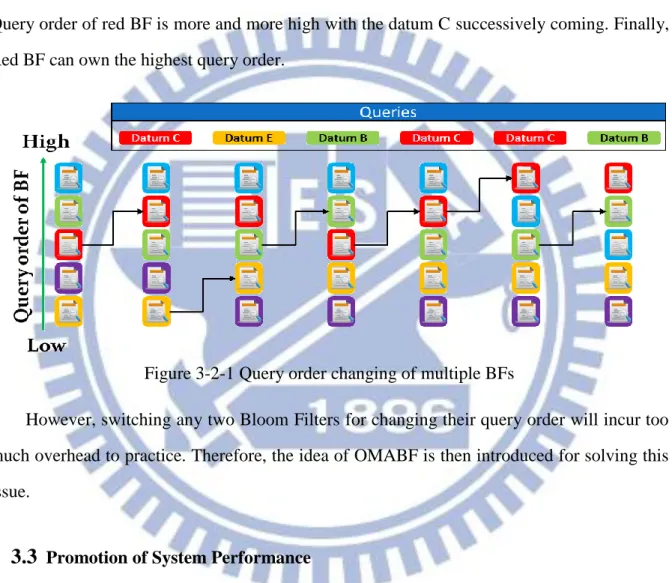
Policy of Changing Query Priority

There is no information that can be used to build relations between data which are set in different Bloom Filters because incoming data are unpredictable. Therefore, an optimal searching scheme does not exist. Fortunately, queried data has feature of temporal locality. The feature of the data can help to filter out which data are more frequently queried. For this reason, query order of the data can be sorted by their popularities. Our policy is considered that the query order of a Bloom Filter can be promoted one level up once the Bloom Filter contains a queried datum for really reflecting the popularity of the datum. A Bloom Filter which contains a large number of queried data must be assigned with higher query order after

has a higher query order. Figure 3-2-1 shows our idea to promote query order of a BF. We take a red color BF as an example. In the beginning, the red BF located in third query order. Then, the BF is promoted one query order when a queried datum C coming. Although other queried data are continuously coming and help to promote they own BF, but the query order just switch between two adjacent BFs. The major factor to promote query order of a BF still depends on the popularity of the BF. In the example, red BF is more popular than others. Query order of red BF is more and more high with the datum C successively coming. Finally, Red BF can own the highest query order.

However, switching any two Bloom Filters for changing their query order will incur too much overhead to practice. Therefore, the idea of OMABF is then introduced for solving this issue.

3.3

Promotion of System Performance

Multiple memory access times are required for membership check of Bloom Filter because bits which are used to represent a datum are randomly distributed to multiple memory blocks. The number of memory access can be reduced if the bits are rearranged to less memory blocks. We replace original Bloom Filters with OMABFs in order to achieve this goal. OMABF takes one or more blocks for setting a datum. The bits are evenly shared by the blocks. Therefore, memory access times can be significantly reduced. Besides, the blocks can be regarded as a tiny Bloom Filter for measuring and managing purposes. Compared with

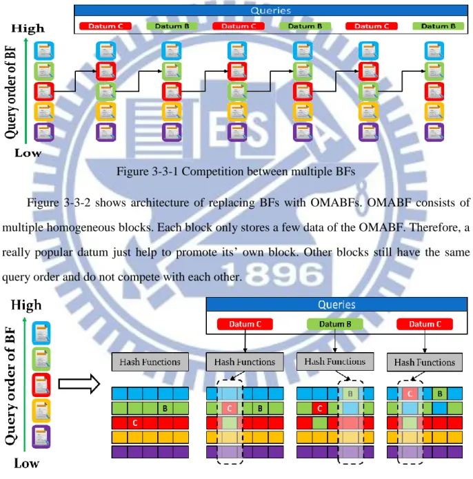
original Bloom Filter, more accurate result of popularity of data can be obtained by measuring the block. In the same time, the blocks can be assigned with different query order respectively. Therefore, the most popular blocks gain higher query order and create better performance. Figure 3-3-1 figure out a phenomenon of competition once more than one BF are popular and have approximate popularity to each other. Queried data keep promoting their own BF and leading the query order of two BFs always exchange. Therefore, the more overhead is caused.

Figure 3-3-2 shows architecture of replacing BFs with OMABFs. OMABF consists of multiple homogeneous blocks. Each block only stores a few data of the OMABF. Therefore, a really popular datum just help to promote its‟ own block. Other blocks still have the same query order and do not compete with each other.

However, the problem of updating Bloom Filter may be caused by switching blocks for changing query order, because no information can be used to trace where a block is. Thus,

Figure 3-3-2 Architecture of replacing BFs with OMABFs Figure 3-3-1 Competition between multiple BFs

actually moving blocks is impractical. A concise data structure is introduced for solving this problem with punishment of little extra memory space.

3.4

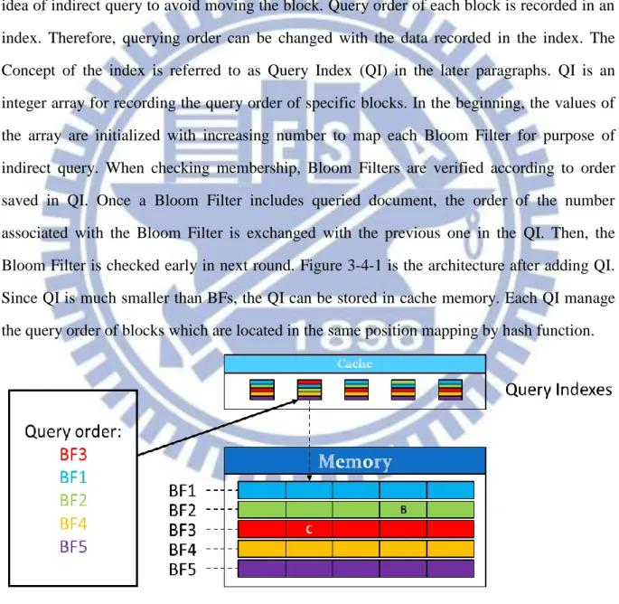
Query Index

Extra overhead is created when moving blocks to change their query order. Two costs are considered: (1) Extra memory access times for exchanging blocks between two Bloom Filters (2) Updating incorrect memory blocks. Based on these considerations, we propose an idea of indirect query to avoid moving the block. Query order of each block is recorded in an index. Therefore, querying order can be changed with the data recorded in the index. The Concept of the index is referred to as Query Index (QI) in the later paragraphs. QI is an integer array for recording the query order of specific blocks. In the beginning, the values of the array are initialized with increasing number to map each Bloom Filter for purpose of indirect query. When checking membership, Bloom Filters are verified according to order saved in QI. Once a Bloom Filter includes queried document, the order of the number associated with the Bloom Filter is exchanged with the previous one in the QI. Then, the Bloom Filter is checked early in next round. Figure 3-4-1 is the architecture after adding QI. Since QI is much smaller than BFs, the QI can be stored in cache memory. Each QI manage the query order of blocks which are located in the same position mapping by hash function.

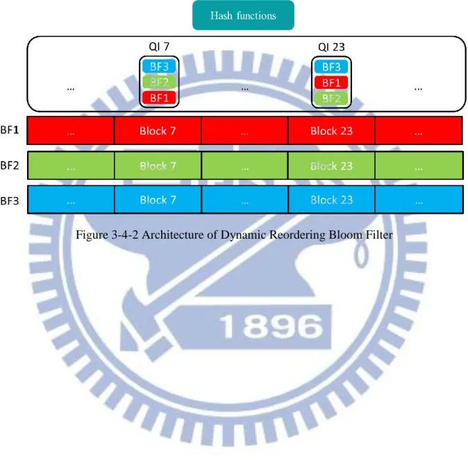
The final architecture of Dynamic Reordering Bloom Filter is shown in Figure 3-4-2. Block hash function is used to choose the blocks which are in the same position but across

many OMABFs when accessing a datum. Each position is represented by different numbers. Query Index which has the same number as the blocks is used to manage the query order of the blocks. The blocks are checked following the number reported by Query Index when querying a datum. Query Index may be modified once a block includes the queried datum.

Chapter 4: System Performance Analysis

Markov chain [19] is a common mathematical model for predicting the probability of a specific serial of states. The model is suitable for predicting our scheme because the probability of forming next query order is decided by a specific serial of states. The average performance of accessing the most popular Bloom Filters in our scheme is predicted by Markov chain and evaluated through simulations to understand the performance under different distributions of bias.

4.1

Markov chain analysis

A Markov Chain is stochastic process with the Markov property on a finite state space. Markov property is defined as that probability of next state occurring depends on the present state and is independent of the past state. Markov property can be formulated as:

)

|

(

)

...

|

(

X

_{n 1}

x

_{n 1}

X

₀

x

₀

X

_n

x

_n

P

X

_{n 1}

x

_{x 1}

X

_n

x

_n

P

_



_







_



_



(3)

The Xn represents the present state. The Xn+1 represents the future state. In our scheme, query

order recorded in QI dominates the cost of membership check in Bloom Filters. Therefore, the evaluation of probabilities for each state of QI can indicate the system performance. Applying Markov chain to evaluate the probabilities needs two input data: (1) an initial states matrix in the QI which we defined as u (2) a transition matrix which we defined as p for recording the probabilities of the transition between any two states. The former depends on which probability of state we would like to predict; the later can be obtained from synthetic or measurement. For calculating purpose, a mathematical model of Markov chain can be formulated as: n n

d

d

p

d

d

p

d

p

d

p

d

d

p

d

d

p

d

p

d

p

d

p

d

p

p

p

d

p

d

p

p

p

u

uP



































































)

1

,

1

(

)

2

,

1

(

...

)

1

,

1

(

)

0

,

1

(

)

1

,

2

(

)

2

,

2

(

...

)

1

,

2

(

)

0

,

2

(

...

...

...

...

...

)

1

,

0

(

)

2

,

1

(

...

)

1

,

1

(

)

0

,

1

(

)

1

,

0

(

)

2

,

0

(

...

)

1

,

0

(

)

0

,

0

(

) ( (4)

0 … 0]. p(a, b) is the probability of state a transits to state b. The number d represents there

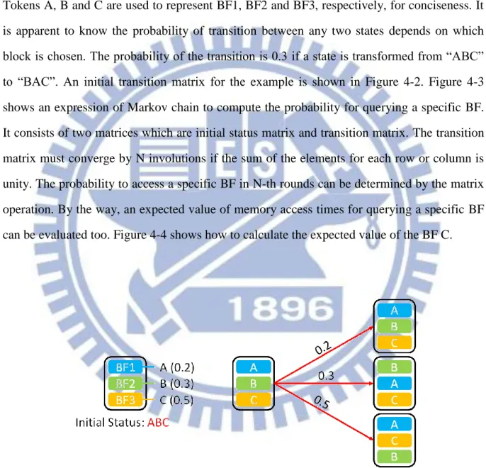
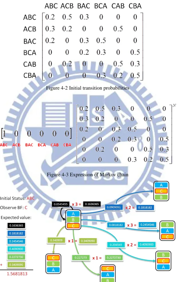
are d states which may be happen. We can predict our scheme performance through the formulation (4). For example, QI maintains query order of three blocks which are from different Bloom Filters. The probabilities to include a queried document for each block are assumed to be 0.2, 0.3 and 0.5. The content of QI for the example is shown in Figure 4-1. Tokens A, B and C are used to represent BF1, BF2 and BF3, respectively, for conciseness. It is apparent to know the probability of transition between any two states depends on which block is chosen. The probability of the transition is 0.3 if a state is transformed from “ABC” to “BAC”. An initial transition matrix for the example is shown in Figure 4-2. Figure 4-3 shows an expression of Markov chain to compute the probability for querying a specific BF. It consists of two matrices which are initial status matrix and transition matrix. The transition matrix must converge by N involutions if the sum of the elements for each row or column is unity. The probability to access a specific BF in N-th rounds can be determined by the matrix operation. By the way, an expected value of memory access times for querying a specific BF can be evaluated too. Figure 4-4 shows how to calculate the expected value of the BF C.

Figure 4-2 Initial transition probabilities

Figure 4-3 Expression of Markov chain

Chapter 5: Simulation Results

This section discusses the performance of our scheme. Firstly, the performance of our scheme for querying the most popular block of ten blocks is discussed. The performance is predicted by Markov Chain and evaluated by simulation. Secondly, four data sets which consist of one artificial and three trace log files are used to evaluate the performance of our scheme.

5.1

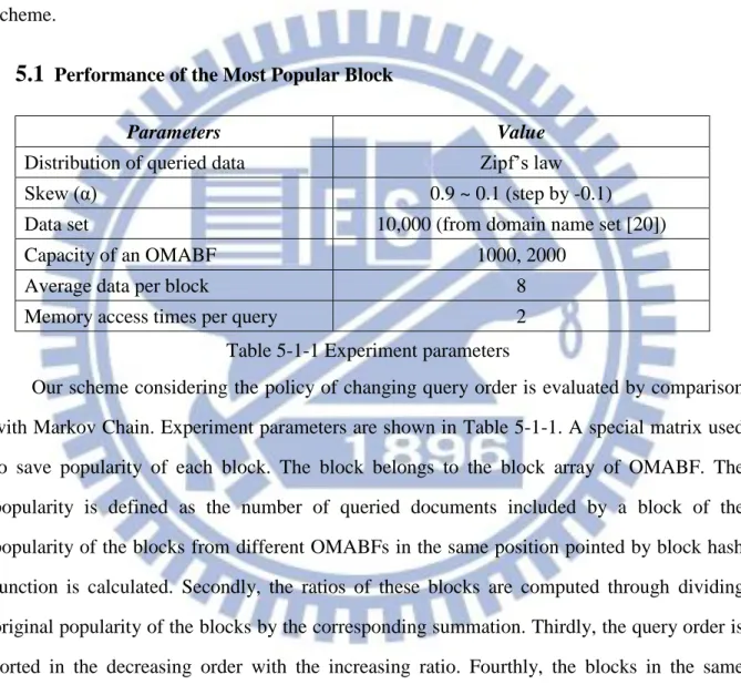
Performance of the Most Popular Block

Parameters Value

Distribution of queried data Zipf‟s law

Skew (α) 0.9 ~ 0.1 (step by -0.1)

Data set 10,000 (from domain name set [20])

Capacity of an OMABF 1000, 2000

Average data per block 8

Memory access times per query 2 Table 5-1-1 Experiment parameters

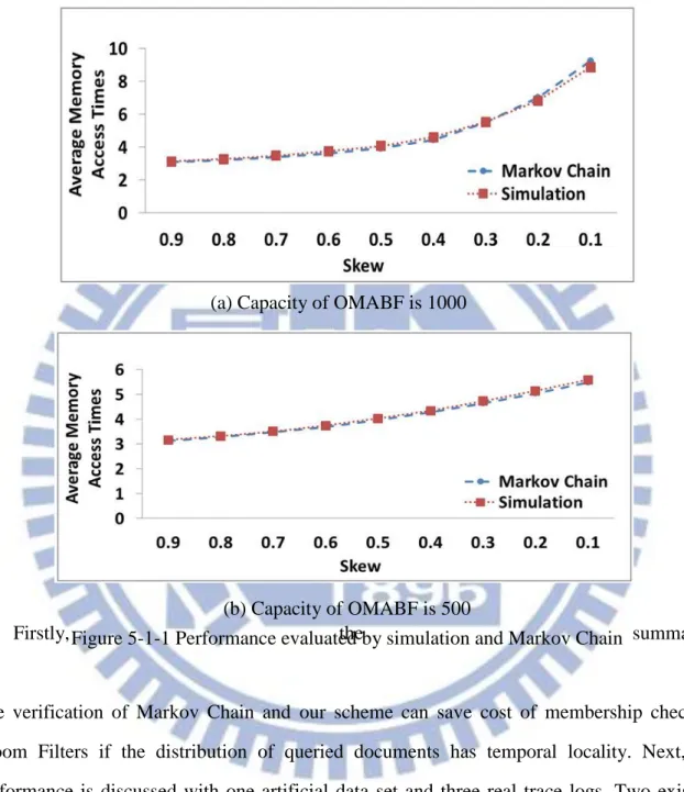
Our scheme considering the policy of changing query order is evaluated by comparison with Markov Chain. Experiment parameters are shown in Table 5-1-1. A special matrix used to save popularity of each block. The block belongs to the block array of OMABF. The popularity is defined as the number of queried documents included by a block of the popularity of the blocks from different OMABFs in the same position pointed by block hash function is calculated. Secondly, the ratios of these blocks are computed through dividing original popularity of the blocks by the corresponding summation. Thirdly, the query order is sorted in the decreasing order with the increasing ratio. Fourthly, the blocks in the same position are regarded as a group for evaluation. Finally, the average expected value of the blocks which are the most popular in each group is estimated by simulation and Markov Chain. The result of the simulation by our scheme is compared with that predicted by Markov Chain as shown in Figure 5-1-1. Obviously, both results show that query cost increase with the decreasing parameter “skew”. The parameter means the degree of bias of popularities. The

bias of popularity is more significant if the value of skew is larger. Therefore, our scheme can reduce the cost of membership check under the effect of the temporal locality.

Firstly, the summation

The verification of Markov Chain and our scheme can save cost of membership check in Bloom Filters if the distribution of queried documents has temporal locality. Next, the performance is discussed with one artificial data set and three real trace logs. Two existing schemes called Dynamic Bloom Filter and Time-Dependent Bloom Filter are taken into account for comparison. In the following content, the noun “dynamic bloom filters” is used for representing DBF, TMBF or DRBF. Each one of dynamic bloom filters uses Bloom-2 Filters to manage their data set. Artificial data shows the performance in dynamic bloom filters under different skew. Threes real trace logs come from different application fields.

(b) Capacity of OMABF is 500

Figure 5-1-1 Performance evaluated by simulation and Markov Chain (a) Capacity of OMABF is 1000

5.2

Artificial Data Sets

Parameters Value

Popularity distribution Zipf‟s law Skew (α) 0.9 ~ 0.5 (step by -0.1) Data set 10,000 (From domain name set [20]) Queried data set 1,000,000 (According to Zipf‟s law)

Capacity of BF 500, 1000

Memory size per datum 30 bits

Memory size of each Query Index 128 bits (5 bits for an OMABF)

Average data per block 8

Memory Size 300000 bits (DRBF、DBF and TMBF) 16,000 bits (In cache for DRBF) Memory access times per query 2

The number of hash functions 21 Table 5-2-1 Parameters for simulation test data

Table 5-2-1 shows parameters used to produce artificial data sets. The base of the data set is downloaded from Open Directory Project [20] maintained by Netscape of American OnLine. There are 3.6 million uniform resource locators (URL) in the set. Ten thousand tested URLs are randomly extracted from the set. The tested URLs are randomly (not duplicate) multiplied with the numbers produced by Zipf‟s law under different skews (called α) for creating queried URLs. Each dynamic bloom filter is assigned with two kinds of Query Depth for verification. Query Depth is defined as the maximum number can be checked for one queried datum. Obviously, DRBF can reduce cost of membership check with increasing α in Figure 5-2-1 (A). When α is 0.9, DRBF reduces at most 46% memory access times for membership check. This is because significant bias distribution makes Popular Bloom Filters in higher query priority occur in higher probability. For other dynamic bloom filters, they have similar performance because the popular queried URLs in the data set are uniformly distributed. At the same time, they execute membership check with sequential search and have no opportunity to gain better performance under bias query distribution. In Figure 5-2-1 (B), DRBF gains more benefit when Query Depth is twenty. However, the improvement of

distribution of queried URLs dominates the performance. When α=0.9, DRBF can reduce at most 50% memory access times.

5.3

NASA Web Server Trace Log File

Parameter Value

Log date July 1, 1995

During 30 days

URL set 15,350 URLs

Queried URL set 1,569,850 URLs Table 5-3-1 Profile of NASA web server trace log

NASA web server trace log is downloaded from [21]. The profile of the log is shown in Table 5-3-1. Fields of the log file are client ID, timestamp, request URL, etc. Data of the request URL field are converted to two data sets called URL set and Queried URL set. The former consists of distinct URLs extracted from log file and are set into dynamic bloom filters. The later is used for querying dynamic bloom filters. Query Depth is set as thirty. Data of

(a) Query Depth is ten

(b) Query Depth is twenty

URL set are evenly set into each Bloom Filter with ascending timestamp order. It is because the number of new URLs seldom appears every day. More than 95% queried URLs appear during the first day. The main reason is that, there are some image files such as logo icon of NASA which appears in most web pages. Others rarely-queried URLs are dynamically created when users interact with web pages. In Figure 5-3-1, TMBF has worse performance under this kind of distribution, because it checks membership from the most recent Bloom Filter to the oldest one. The idea is not appropriate for the application in web servers. On the contrary, DBF checks membership from the oldest Bloom Filter to the most recent one. The idea perfectly matches the distribution and gains significant benefit. Our scheme also gains large benefit because the distribution has extreme high degree of bias.

5.4

eDonkey tracker trace log file

Parameter Value

Log date November 1, 2006

During 27 day

URL set 2,307,512 file hash codes Queried URL set 2,335,718 URLs

Table 5-4-1 Profile of eDonkey trace log file

Trace log file is downloaded from [22]. The log file records events of peers which communicate with server. We sample 1% of the file hash codes from the log file to verify the performance of dynamic bloom filters. File hash code is a MD5 hash code for representing the

signature of a file piece which is requested or shared by the peers. Two data sets are created from the 1% file hash codes. The first data set stores file hash codes which are not repeated. The second data set stores the full sample data. The profile of the sample data is shown in Table 5-4-1. Query Depth is set as twenty-seven because date of the file hash codes which is firstly discovered is uniformly distributed over every day. The distribution has a serious appearance of bias. TMBF gains large benefit from the distribution because of its membership check scheme. Similarly, our scheme also gains large benefit because our scheme uses the same query priority as TMBF. Verification of the log file is shown in Figure 5-4-1.

5.5

Web Proxies Log Files

Parameter Value

Log date January 9, 2007

During 1 day

URL set 296,269 URLs

Queried URL set 1,415,075 URLs Table 5-5-1 Profile of web proxies trace log files

Trace log files are downloaded from [23]. These log files are created by web proxies in the United States. The format of these files follows Squid. Data is extracted for verifying the performance of dynamic bloom filters if the result code [24, section 6.7] includes the key word “HIT” but excludes a key word “TCP_NEGATIVE_HIT”. The latter representing a queried web document does not exist in the cache. Otherwise, web proxy has the

corresponding document in cache. The profile of these trace log files is shown in Table 5-5-1. In this paragraph, eight trace log files are mixed and reallocated to eight Bloom Filters. Each group is assigned 37,034 URLs for simulating the operation of cooperative web proxy. The performance of the dynamic bloom filters is shown as Figure 5-5-1. In the experiment, the order of queried URLs is the same as trace log files. URLs set into dynamic bloom filters are randomly distributed. Eight Bloom Filters at most need to be checked when executing membership check for a queried URL. The performance is similar to the first experiment. Our scheme has better performance than the other two. For the same reason, the distribution of queried data has feature of temporal locality. At most 43% cost of membership check is saved.

5.6

Changing of False Positive Ratio of Bloom-g Filter

Parameter Value

Popularity distribution Random

Data set 30,720 (From domain name set [20]) Queried data set 3,072,000 (exclude data set) Capacity of a BF Randomly selecting from [20] The number of blocks per datum 1024、1536 and 3072

The number of blocks 2、3 and 4

Table 5-6-1 False Positive Ratio of N-MABF for Different Number of Block

Bloom-1 Filter is very effective for accessing Bloom Filters. However, the false positive ratio is very large because data are non-uniformly set to each block. Therefore, Bloom-g Filter is proposed to solve this problem. The false positive ratio decreases with the number of the

blocks dividing k independent hash functions. When the number is two, the false positive ratio is significantly improved. The effect of the number of the blocks on the false positive ratio declines once the number is larger than two. The improved performance is shown as Table 5-6-2.

Value of N False Positive

ration of 10 N

False positive ratio of 20 N

False positive ratio of 30 N

2 1.65E-04 3.26E-04 5.02E-04

3 2.95E-05 4.20E-05 6.43E-05

4 2.54E-05 3.22E-05 4.52E-05

Chapter 6: Conclusions

Bloom Filter provides the benefits of space-efficient and constant time to execute membership check. The applications of Bloom Filter to filter incoming data improve system performance by avoiding irrelevant data. However, using Bloom Filters to manage the information of distributed system may suffer from membership check in many Bloom Filters. The average searching cost of Bloom Filters increases with the number of cooperative peers. This thesis focused on this issue and proposed a concise scheme for reducing the average cost of membership check. With the temporal locality characteristic in web requests, popular queried documents can be assigned with higher query priority in checking multiple Bloom Filters. We use three real trace logs from NASA web server, edonkey tracker server and web proxies to comparing the performance of our scheme with linear and reverse query order. Our scheme always have better performance. That is because our scheme can immediately change the query order of a BF once it is hit by a queried datum. Hence, search cost of popular data can be rapid dropped down and save more memory access times.

References

[1] B. H. Bloom, "Space/time trade-offs in hash coding with allowable errors," presented at the Communications of the ACM, 1970.

[2] L. Li, et al., "A variable length counting Bloom filter," in Computer Engineering and Technology (ICCET), 2010 2nd International Conference on, 2010, pp. V3-504-V3-508. [3] F. Bonomi, et al., "An improved construction for counting bloom filters," in

Algorithms–ESA 2006, ed: Springer, 2006, pp. 684-695.

[4] D. Ficara, et al., "Multilayer compressed counting bloom filters," in INFOCOM 2008. The 27th Conference on Computer Communications. IEEE, 2008, pp. 311-315. [5] M. Mitzenmacher, "Compressed bloom filters," presented at the IEEE/ACM

Transactions on Networking (TON), 2002.

[6] H. Song, et al., "Ipv6 lookups using distributed and load balanced bloom filters for 100gbps core router line cards," in INFOCOM 2009, IEEE, 2009, pp. 2518-2526.

[7] S. Dharmapurikar, et al., "Longest prefix matching using bloom filters," in Proceedings of the 2003 conference on Applications, technologies, architectures, and protocols for computer communications, 2003, pp. 201-212.

[8] K. Shanmugasundaram, et al., "Payload attribution via hierarchical bloom filters," in Proceedings of the 11th ACM conference on Computer and communications security, 2004, pp. 31-41.

[9] P. Jokela, et al., "LIPSIN: line speed publish/subscribe inter-networking," in ACM SIGCOMM Computer Communication Review, 2009, pp. 195-206.

[10] P. B. Danzig, et al., "A case for caching file objects inside internetworks," 1993.

[11] L. Fan, et al., "Summary cache: a scalable wide-area web cache sharing protocol," presented at the IEEE/ACM Transactions on Networking (TON), 2000.

[12] Y. Qiao, et al., "One memory access bloom filters and their generalization," in INFOCOM, 2011 Proceedings IEEE, 2011, pp. 1745-1753.

[13] D. Guo, et al., "The dynamic bloom filters," presented at the Knowledge and Data Engineering, IEEE Transactions on, 2010.

incremental set," presented at the Ultra Modern Telecommunications & Workshops, 2009. ICUMT'09. International Conference on, 2009.

[15] S. Jin and A. Bestavros, "Sources and characteristics of Web temporal locality," in Modeling, Analysis and Simulation of Computer and Telecommunication Systems, 2000. Proceedings. 8th International Symposium on, 2000, pp. 28-35.

[16] A. Mahanti, et al., "Temporal locality and its impact on Web proxy cache performance," presented at the Performance Evaluation, 2000.

[17] L. Breslau, et al., "Web caching and Zipf-like distributions: Evidence and implications," in INFOCOM'99. Eighteenth Annual Joint Conference of the IEEE Computer and Communications Societies. Proceedings. IEEE, 1999, pp. 126-134.

[18] P. Cao and S. Irani, "Cost-Aware WWW Proxy Caching Algorithms," in Usenix symposium on internet technologies and systems, 1997, pp. 193-206.

[19] Hoel, P., Port, S., Stone, C.,《Introduction to Stochastic Processes》, Houglition Mifflin, 1972.

[20] Open Directory Project. Available: http://rdf.dmoz.org/ [21] NASA web server trace log file. Available:

http://ita.ee.lbl.gov/html/contrib/NASA-HTTP.html

[22] eDonkey trace log file. Available: http://fabrice.lefessant.net/traces/edonkey2/

[23] Web proxies trace log files. Available: ftp://ftp.ircache.net/Traces/DITL-2007-01-09/ [24] Squid. Available: http://www.comfsm.fm/computing/squid/FAQ-6.html