國 立 交 通 大 學
電子工程學系 電子研究所
碩
士
論
文
基於深度卷積神經網路之
手勢辨識技術研究
Hand Gesture Recognition based on
Deep Convolutional Neural Network
研
究
生:謝汝欣
指 導 教 授:王聖智 教授
基於卷積深度神經網路之
手勢辨識技術研究
Hand Gesture Recognition based on
Convolutional Deep Neural Network
研 究 生:謝汝欣 Student:Ju-Hsin Hsieh
指 導 教 授:王聖智 教授 Advisor:Prof. Sheng-Jyh Wang
國 立 交 通 大 學
電子工程學系 電子研究所碩士班
碩 士 論 文
A ThesisSubmitted to Department of Electronics Engineering & Institute of Electronics College of Electrical and Computer Engineering
National Chiao Tung University in partial Fulfillment of the Requirements
for the Degree of Master of Science in
Electronics Engineering
August 2014
Hsinchu, Taiwan, Republic of China
基於深度卷積神經網路之手勢辨識技術研究
研究生:謝汝欣 指導教授:王聖智 教授
國立交通大學
電子工程學系 電子研究所碩士班
摘要
在這篇論文中,我們提出了一個使用任意單一攝影機在不同角度下仍能遠距離辨識 多重手勢的技術。此技術不需固定攝影機角度,不需要由特定使用者操作,且能分辨多 種手勢。此技術在影片中自動找出使用者的手的位置,並判斷使用者想傳達的訊息,希 望能進行遠距離的操作以及在任何背景之下皆能達到手勢辨識的效果。在此設定議題下, 為了能在複雜背景與不同視角拍攝的情況下有效的找到手部出現的區域以及辨識使用 者所傳達的訊息,我們不採用易被複雜背景所誤導膚色資訊且不使用事先設定之特徵萃 取技術,而是利用卷積神經網路有效且準確的學習不同手勢所擁有的特徵,並結合不同 形狀與大小的特徵,以找到能分離不同手勢最佳的特徵空間,再利用深度神經網路找出 特徵之間的關係以及不同手勢與各特徵的連接,藉此達到手部偵測與多重手勢辨識的成 果。此外,我們也利用影片中已經得到的手部位置與移動資訊加上手勢辨識結果,推測 之後較有可能出現手部的區域以及最佳的手勢辨識結果。Hand Gesture Recognition based on
Deep Convolutional Neural Network
Student:Ju-Hsin Hsieh Advisor:Prof. Sheng-Jyh Wang
Department of Electronics Engineering, Institute of Electronics
National Chiao Tung University
Abstract
In this thesis, we propose an algorithm which recognize hand gestures with a single camera
under different view-points within a range remotely. The algorithm can recognize
multi-gestures without fixing view-point of the camera or a particular user controlling. In order to
find the hand position and recognize the gestures from the video automatically and efficiency
in the clutter background under different view-points within a range, we don’t take the skin
color as the information which is easily influence by the clutter background, nor do we use the
specific feature extraction processing. Instead, we use the convolutional neural network to learn
the features in the hand gesture image and combine the different kernel sizes to get the best
feature space for separating different gestures. Then we use the deep neural network to find the
relationship between the hand features and the gesture classes. Under this setting, we are able
to locate the hand and recognize multi hand gestures. Furthermore, with the help of the temporal
information for the hand position and motion getting from the video, we are able to infer the
Content
Chapter 1.
Introduction ... 1
Chapter 2.
Related Works ... 3
2.1 Hand Gesture Recognition by using Random Forest ... 3
2.2 Hand Gesture Recognition by Neural Network ... 6
Chapter 3.
Proposed Method ... 9
3.1 Data Set ... 11
3.1.1 Data set for Convolutional Neural Network ... 11
3.1.2 Data set for Deep Neural Network ... 12
3.2 Basic concept of two learning algorithm ... 14
3.2.1 Convolutional Neural Network ... 14
3.2.2 Deep Neural Network ... 20
3.3 Applicable to Hand Gesture Recognition ... 24
3.3.1 Feature Extraction by Convolutional Neural Network ... 25
3.3.2 Deep Convolutional Neural Network Classification ... 34
3.3.3 Tracking Technique ... 36
3.4 Refinement ... 40
Chapter 4.
Experimental Results ... 43
4.1 Detection accuracy ... 43
4.2 Combine Tracking and Detection ... 46
4.3 Video comparison ... 49
List of Tables
Table 3-1 Different kernel size correspond to different pooling scaling factor. ... 28
Table 4-1 Accuracy rate for training data set. ... 44
Table 4-2 Accuracy rate for testing data set. ... 44
Table 4-3 The computing time for detection only and detection combine tracking... 47
Table 4-4 The hand gesture recognition accuracy for detection only and detection combine tracking of video 1. ... 47
Table 4-5 The hand gesture recognition accuracy for detection only and detection combine tracking of video 2. ... 48
Table 4-6 The hand gesture recognition accuracy for our proposed deep convolutional neural network, traditional convolutional neural network and traditional deep neural network of video 1. ... 50
Table 4-7 The hand gesture recognition accuracy for our proposed deep convolutional neural network, traditional convolutional neural network and traditional deep neural network of video 2. ... 50
List of Figures
Figure 2-1 Eight edge filters and the corresponding edge maps for the image “Five”. ... 4 Figure 2-2 Compare traditional grid cells and randomized pooling cells for hand image. ... 5 Figure 2-3 (a) Training procedure of random forest with randomized pooling cells.
(b) The final trained random pooling cells for hand image. ... 6 Figure 2-4 Overview of hand gesture recognition system... 7 Figure 2-5 (a) Central coordinates normalization. (b) Example of general features matrix. ... 7 Figure 3-1 (a) Training procedure of our proposed algorithm.
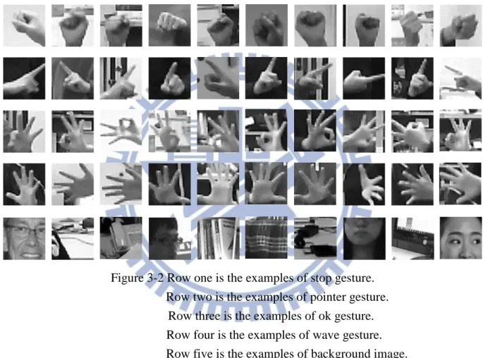
(b) Testing procedure of our proposed algorithm. ... 11 Figure 3-2 Row one is the examples of stop gesture.
Row two is the examples of pointer gesture. Row three is the examples of ok gesture. Row four is the examples of wave gesture.
Row five is the examples of background image. ... 12 Figure 3-3 For each row, there are, 3*3, 6*6, 7*3 and 3*7, four different kinds of kernel size. For each column, there are stop, pointer, ok, wave and background five different kinds of input images. . 13 Figure 3-4 Example of convolutional neural network architecture. ... 15 Figure 3-5 (a) An example of input image.
(b) Neural network : A hidden node with its fully-connected weight which might learns from the input image data set.
(c) Convolutional neural network : A hidden node with its local-connected weight which might learns from the input image data set. ... 16 Figure 3-6 (a) An example of a specific kernel.
(b)&(c) Two different input image with same appearance but some local translation feature (as circled region).
(d)&(e) Two feature map corresponding to two input image and its pooling result. ... 17
Figure 3-8 (a) Architecture of MCMC by using Gibbs sampling.
(b) Architecture of Contrastive Divergence algorithm ... 24 Figure 3-9 (a) The kernel of convolutional neural network is a small square.
(b) The kernel of convolutional neural network is a large square. (c) The kernel of convolutional neural network is a long and narrow stipe. ... 26 Figure 3-10 (a) The convolutional neural network feature learned by 3*3 kernel size.
(b) The convolutional neural network feature learned by 6*6 kernel size. (c) The convolutional neural network feature learned by 7*3 kernel size.
(d) The convolutional neural network feature learned by 3*7 kernel size. ... 27 Figure 3-11 (a) The feature map of kernel 3*3, red circled region show the rough contour of hand
gestures.
(b) The feature map of kernel 6*6, red circled region show the rough contour of hand gestures.
(c) The feature map of kernel 7*3, red circled region show the finger feature.
(d) The feature map of kernel 3*7, red circled region show the finger feature. ... 31 Figure 3-12 The different kernel size we need for hand gesture images. ... 32 Figure 3-13 (a) Four of sixteen kernels we choose and corresponding feature maps for stop, pointer, ok
and wave gestures.
(b) Four specific kernels and corresponding feature maps for stop, pointer, ok and wave gestures. ... 32 Figure 3-14 (a) The schematic diagram of feature space which is easy to separate.
(b) The schematic diagram of feature space which is not easy to separate. ... 34 Figure 3-15 The feature vectors combining different kernel size for the hand gestures. ... 34 Figure 3-16 (a) Our deep neural network model architecture.
(b) The example of the activation function after the hidden node. ... 35 Figure 3-17 (a) The example of point tracking method.
(b) The example of kernel tracking method.
(c) The example of silhouette tracking method. ... 37 Figure 3-18 An example for the detection region adjustment and the motion estimation result... 38 Figure 3-19 The example of target patch and three testing patch with its two dimension correlation for the target patch. ... 39
Figure 3-20 The examples for the position map and the motion map. ... 40 Figure 3-21 (a) The flowchart for the weight score of detection result.
(b) The flowchart for the weight score of tracking result. ... 41 Figure 3-22 The example of the temporal information refinement of our proposed method. ... 42 Figure 4-1 (a) Example frames for our proposed method, convolutional neural network and deep
neural network in a row of video 1... 46 Figure 4-2 (a) Example frames for detection only algorithm and detection combine tracking algorithm
in a row of video 1.
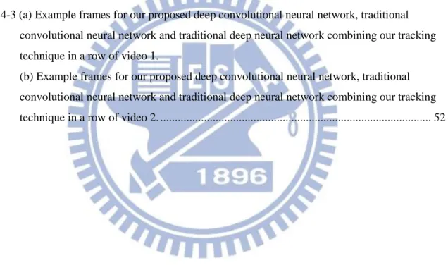
(b) Example frames for detection only algorithm and detection combine tracking algorithm in a row of video 2... 49 Figure 4-3 (a) Example frames for our proposed deep convolutional neural network, traditional
convolutional neural network and traditional deep neural network combining our tracking technique in a row of video 1.
(b) Example frames for our proposed deep convolutional neural network, traditional convolutional neural network and traditional deep neural network combining our tracking technique in a row of video 2. ... 52
Chapter 1. Introduction
In the technological era, computers play an important role in our daily lives. Our most
common way to communicate with computer is through the mouse and keyboard. However, we
want to interact with computer directly instead of using mechanical devices. The progress of
computer vision and machine learning algorithms enable us to interact with computer in novel
ways, such as Kinect. We can use our hand gesture to convey our thought intuitively.
Hand gesture recognition system can be categorized into three stages: detection, tracking
and recognition. We want to know the position of our hand in an image, then track the
movement of hand and the moving trajectory. Finally, the computer must understand the
meaning of user expression. Traditionally, people usually find skin color in the image with
simple background and investigate the appearance of skin color part to determine where the
hand is. Based on the temporal information obtained from acquired trajectory and result, predict
the hand movement. At last, we use some classification methods to identify the gesture we
express. However, the variant of appearance of hand is complicated since our hand is composed
of five fingers and a palm. In addition, a finger has two knuckles to change the exterior of our
hand. Furthermore, the shape of hand will be significantly different as the view point is
changing. If the image has a complex background, it will influence the result of hand gesture
recognition. Therefore, finding a robust classifier against complex background is difficult when
using a simple model. Traditional machine learning method like support vector machine and
random forest may not apply to multiple hand gestures and out-of-plane rotation of hand. As
with the rapid development of deep learning algorithm, we want to use deep learning algorithm
to find a robust classifier of hand gesture.
In this thesis, we want to identify four different gestures, stop, pointer, ok and wave in the
which the detection and recognition stage is based on convolutional neural network and deep
neural network. These two methods are widely used in handwritten digit recognition recently.
We modify the convolutional neural network to apply it to the hand gesture data set. Combining
convolutional neural network and deep neural network to build our classification model for
multiple hand gestures and the hand detector. Due to the dramatic change of hand shape and
appearance, the points to track are not easy to choose. Therefore, nowadays tracking algorithms
are not robust of hand tracking. Therefore, we rely on the detection achievement and adding
some basic tracking technique to improve the detection accuracy and reduce the computation
time.
In our algorithm, we first use convolutional neural network [1]錯誤! 找不到參照來源。
to extract the feature of an image, and transform RGB images to the feature space. Then use
these features of hand as the input of deep neural network. At deep neural network stage, we
use unsupervised learning method : Restricted Boltzmann Machine (RBM) [3] to pre-train the
relationship within the low level local features. Combine the local features into global features
at RBM training stage. Then add labeled data to do the supervised fine-tuning stage to get the
classification model. After we get the hand position in the frame and the gesture it represents,
we can only search for the neighbor region to find the hand position in the next frame. In order
to improve the accuracy, we calculate the patch similarity of adjacent region to correct the
position of the hand. After we get the detection and tracking results, we will do some refinement
to get the most reliable position and gesture class in the video frame.
The thesis is organized as follows. We will introduce some other hand gesture recognition
Chapter 2. Related Works
The main purpose of hand gesture recognition is to convey user’s expression for the
computers. The rapid development of vision based hand gesture recognition increase the
possibility of remote control human computer interface. There are two different ways to do the
hand gesture recognition. One way is using some additional equipment to help doing the
recognition, such as Microsoft Kinect and the MIT colored glove. Another way is using the
appearance of hand to classify different gestures in which extracting some specific feature in
the image. The classification accuracy has been strongly associated with the feature extraction.
In this section, we introduce two different methods of using the appearance of hands to
recognize different gestures. The first method introduced in section 2.1 extracts different
orientation edges from hand images and trains the classification model by the random forest
algorithm. In section 2.2, the second method extracts the hand contour and complex moments
in hand images as the feature vector. They use the neural network algorithm to classify the
images into different hand gestures.
2.1 Hand Gesture Recognition by using Random Forest
In [10], they propose a single-camera hand gesture recognition algorithm forhuman-computer interface. The hand gesture recognition algorithm is composed of three parts. First,
they us eight pre-defined edge filters to generate the corresponding edge maps for the hand
images. Second, they use randomized pooling cell method to learn more efficient cells for the
hand images. They get image feature vectors by concatenating feature vectors in some different
size and shape cells. Finally, they use these feature vectors to train a random forest model for
At first, they use 360∘orientation edge filters to generate the corresponding edge maps
for the hand images. They quantize 360 degrees into 8 bins, then get eight filtered images for
all edge filters. The eight edge filters and the examples of the corresponding edge maps for an
hand image are shown in Figure 2-1.
Figure 2-1 Eight edge filters and the corresponding edge maps for the image “Five”.
After generating the edge maps, they use the structure of randomized pooling cells to
calculate feature vectors [9]. Unlike tradition grid cells, they use more efficient cells to calculate
the edge information for the hand images. Figure 2-2(a) shows traditional grid cells for the hand
image. It partitions the image into equal size and extract the edge information in each cell.
the edge information more efficient for the hand image. After that, the feature vectors of hand
images are concatenated by the feature vectors in all cells.
Figure 2-2 Compare traditional grid cells and randomized pooling cells for hand image.
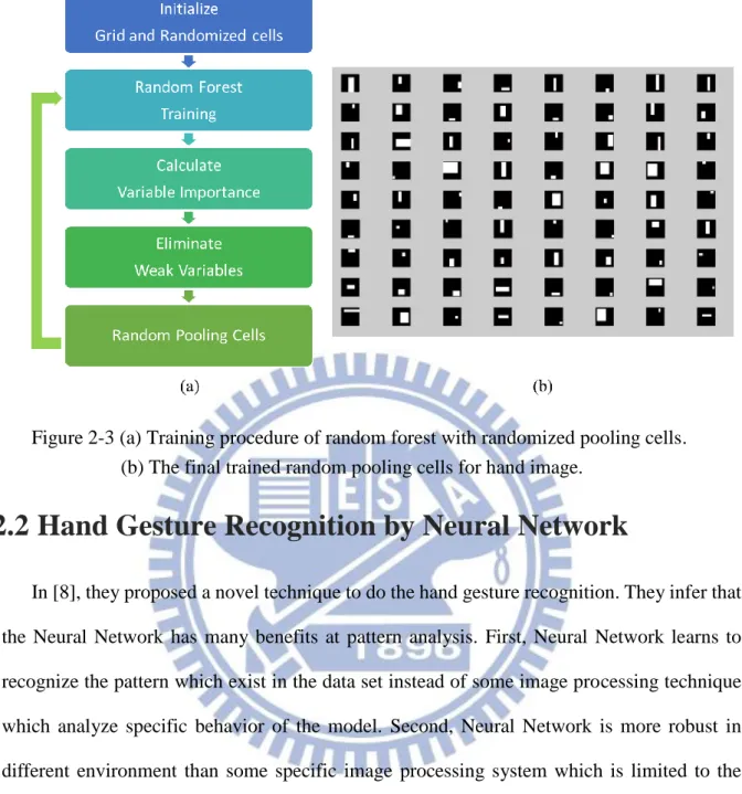
As mentioned in [9], their proposed method of random forest with randomized pooling
cell training procedure is shown in Figure 2-3(a). First, they choose some grid cells and some
randomized cells. Use these cells to calculate the feature vector of hand images and train the
hand gesture classifier by random forest. After that, they calculate the variable importance at
the training stage for the feature vectors and eliminate some weak variables. They eliminate
weak variables and resample different rectangular to get more informative cells iteratively.
Finally, they can get the most efficient cells to extract the edge information from hand images.
Figure 2-3(b) shows the final randomized pooling cells by random forest training stage.
This hand gesture recognition is good at two class recognition. It can classify the “five”
gesture with background and the “zero” gesture with background respectively. The error rate
for two class recognition is about 1 to 2 percent. However, it might get much higher error rate
when the hand gesture classes increased. The error rate for three class recognition may be 5
percent or higher. Therefore, we want to obtain a more robust multi-gesture classifier for hand
Figure 2-3 (a) Training procedure of random forest with randomized pooling cells. (b) The final trained random pooling cells for hand image.
2.2 Hand Gesture Recognition by Neural Network
In [8], they proposed a novel technique to do the hand gesture recognition. They infer that
the Neural Network has many benefits at pattern analysis. First, Neural Network learns to
recognize the pattern which exist in the data set instead of some image processing technique
which analyze specific behavior of the model. Second, Neural Network is more robust in
different environment than some specific image processing system which is limited to the
situation they were designed.
The hand gesture recognition process consist three stages: pre-processing, feature
extraction and classification. Furthermore, they consists of two phases: training (learning) and
classification (testing). Overview of gesture recognition system is seen as Figure 2-4. They
Figure 2-4 Overview of hand gesture recognition system.
At pre-processing stage, they segment the input image into background and objects at first.
They use a thresholding algorithm for segmentation of hand gesture images [13]. In order to
eliminate some errors produced by segmentation algorithm, they use a median filter to reduce
noise. Furthermore, for geometric feature (hand contour), they use edge detection to extract the
hand contour For invariant feature (complex moments), they use image trimming to eliminate
redundant margins and image scaling combine coordinate normalization to let the origin point
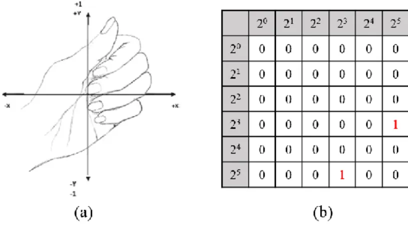
coordinates be at the center of the image as shown in Figure 2-5(a).
At feature extraction stage, for the first method, they extract hand contour by edge map.
Then do the feature image scaling to get an 32*32 image and shift the hand gesture section to
the origin point. Furthermore, they use general feature to be an additional information for height
and width offset of the hand gesture image. Figure 2-5(b) shows the example of height and
width offset matrix, which the hand gesture has the width near to 23 and the height near to 25.
For the second method, they calculate the complex moments from zero-order to ninth-order for
each hand gesture image.
At the last stage, that is classification stage, they use a simple one hidden layer neural
network with back-propagation learning algorithm. Input layer has 1060 nodes or 10 nodes for
two method. Hidden layer has 100 nodes and output layer, the recognition layer, has 6 nodes
for 6 different hand gestures. The recognition rate is 70.83% for the first method and 86.38%
for the second method.
This paper introduce a simple neural network training for hand gesture recognition. It also
pointed out the advantage of learning algorithm. However, this paper still use some image
processing like edge detection to get the feature of data set. In our method, we use convolutional
neural network to extract feature from training data set. It might get more robust recognition
Chapter 3. Proposed Method
The purpose of our system is to detect the hands position and recognize the meaning of
user represent in a video captured by arbitrary camera and viewpoints within a range. The most
difficult part is the clutter background and multi-class gestures classification. We want to figure
out four different kinds of hand gestures: stop, pointer, ok and wave. Because of the complex
background which might have some other skin color like objects with the remote distance of
hand and camera, we won’t use the skin color clue to do the image pre-processing. To build a more robust hand gesture recognition model, our training data is from arbitrary viewpoints
within a range, different users and clutter background. Furthermore, we extract the feature in
training data set by learning features from convolutional neural network, instead of specific
pre-defined image processing technique like edge, corner, contour and silhouette. In order to find
the relationship between local features extract from convolutional neural network, we use the
unsupervised learning algorithm, deep neural network to recognize four different hand gestures.
First find the internal structure in the local features and combine low level features into high
level features at pre-training stage. After that, find the relationship between input features and
output targets at fine-tuning stage. Furthermore, in order to solve the extremely variant shape
of hand gestures, we modify the convolutional neural network to applicable to the multi-class
hand gestures. At testing stage, we add some tracking technique to assist the detection result in
correcting the hand position in the video frame. We also do some refinement to improve our
hand gesture recognition accuracy.
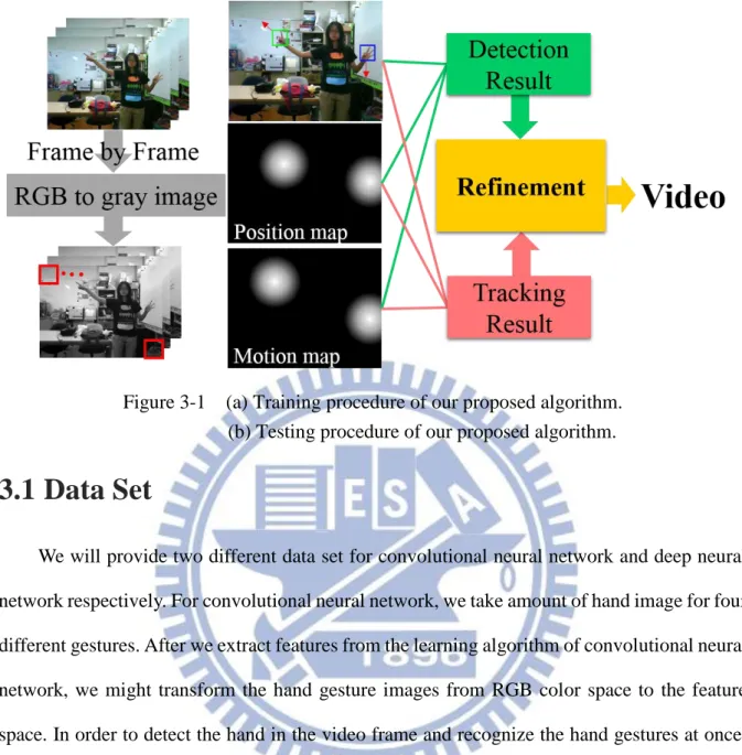
The overall proposed algorithm procedure is shown in Figure 3-1, Figure 3-1(a) shows the
training stage of proposed algorithm and Figure 3-1(b) shows the testing stage of proposed
algorithm. In training stage, we have three steps, learning features, feature combination and
two model we get from training stage but also combining the detection and tracking result to
correct the recognition result.
We will describe the data set we use for convolutional neural network (CNN) and deep
neural network (DNN) in Section 3.1. In Section 3.2, we will describe the learning algorithm
of convolutional neural network and deep neural network, which we need to learn the features
in hand gesture data set and classify different gestures in feature space. We do some
modification for the hand gesture data set at the feature extraction stage by using convolutional
neural network. In Section 3.3, we will introduce our modification and how to combine the
convolutional neural network and deep neural network for doing the hand gesture recognition.
Also, we will add some tracking technique to improve the hand gesture recognition accuracy in
video testing. At last, in Section 3.4, we will use the temporal information and compare the
Figure 3-1 (a) Training procedure of our proposed algorithm. (b) Testing procedure of our proposed algorithm.
3.1 Data Set
We will provide two different data set for convolutional neural network and deep neural
network respectively. For convolutional neural network, we take amount of hand image for four
different gestures. After we extract features from the learning algorithm of convolutional neural
network, we might transform the hand gesture images from RGB color space to the feature
space. In order to detect the hand in the video frame and recognize the hand gestures at once,
we also transform the background from the RGB color space to hand gesture’s feature space.
The training data set for deep neural network will be the feature space of both hand gesture
image and background images.
3.1.1 Data set for Convolutional Neural Network
We take images from arbitrary camera, viewpoints within a range and different clutter
background. The image size is 50*50 pixel by pixel for all gestures. We use particle filter to
automatically extract the hand part in the image. This makes a lot of mistakes, so that we choose
one finger to represent pointer meaning, three fingers to represent ok meaning and all fingers
with the palm to represent wave meaning. In order to have the same number of right hand image
and left hand image, we flip all the hand image we have. Each gestures have 6400 hand images
for training data set, in other words, there are 25600 hand images. We have 3742 hand images
for testing data set. Figure 3-2 are ten examples of hand gesture image in the training data set
for each gestures and the last row are examples of background image for deep neural network.
Figure 3-2 Row one is the examples of stop gesture. Row two is the examples of pointer gesture.
Row three is the examples of ok gesture. Row four is the examples of wave gesture. Row five is the examples of background image.
3.1.2 Data set for Deep Neural Network
After we extract the feature from convolutional neural network, we add the background
features, each column illustrate the same gestures. The order for the gestures are stop, pointer,
ok and wave. The last column is the background image’s features. Each row represent the same kernel size for feature extraction in convolutional neural network. There are 3*3, 6*6, 7*3 and
3*7 four different kinds of kernel size represented in sequence.
Figure 3-3 For each row, there are, 3*3, 6*6, 7*3 and 3*7, four different kinds of kernel size. For each column, there are stop, pointer, ok, wave and background five different kinds of input images.
3.2 Basic concept of two learning algorithm
We will introduce two learning algorithm we need for feature extraction and hand gesture
classification. We will describe the architecture of the learning algorithm at first. After that, we
will explain the basic concept of the learning algorithm.
3.2.1 Convolutional Neural Network
Convolutional neural network is a learning procedure which can extract some regular
pattern or specific feature in a large amount of image which called training data set. The main
idea of convolutional neural network is shared weight and translation invariance. Traditional
neural network connect all input nodes with all hidden nodes. Therefore, when input image has
a corner at left top and a corner at right bottom will make large difference for the learning
weight. Convolutional neural network pose the shared weight concept to learn some regular
pattern in the image. When image has repeated feature, the model might learn only one feature
to represent it. Furthermore, convolutional neural network add a pooling layer after a
convolutional layer, which can let the model be confronted with translation invariance. The
pooling layer calculate the mean of no overlap patch in the feature map which is represent the
appearance probability of feature. In section 3.2.1.1, we will introduce the architecture of
convolutional neural network and describe each layer in detail. We will also brief introduce the
basic learning algorithm of convolutional neural network in section 3.2.1.2.
3.2.1.1 Architecture of Convolutional Neural Network
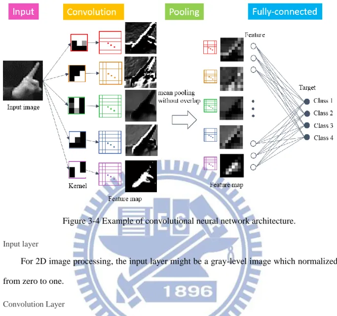
Convolutional neural network has four different type of layers: input layer, convolution
layer, pooling layer and fully-connected layer. Figure 3.4 is an example of convolutional neural
Figure 3-4 Example of convolutional neural network architecture.
Input layer
For 2D image processing, the input layer might be a gray-level image which normalized
from zero to one.
Convolution Layer
In convolution layer, we can assume the number of kernel we need to learn in the image
training data set. Traditional neural network will fully connect all input layer with a hidden
node. A hidden node which connect with all input nodes represent the image appearance. The
larger value the hidden node is, the more similar between input image and weight appearance.
Figure 3.5(a) shows an input image as an example. If we want the hidden node can represent
the input image appearance, the weight appearance might be complex, which shows in Figure
3.5(b). However, convolutional neural network use shared weight to represent regular pattern
arise from input image. A hidden node only connect a local patch in the image and let the node
connected weight, which called kernel, to shows the local feature learn from the input image.
the whole image. Do the convolution function between input image patch and kernel, the larger
the result value, the more similar between local patch and kernel appearance. Figure 3.2(c)
shows an example of a specific kernel and its correspondence feature map.
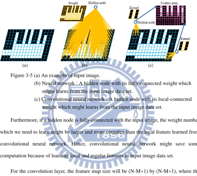
Figure 3-5 (a) An example of input image.
(b) Neural network : A hidden node with its fully-connected weight which might learns from the input image data set.
(c) Convolutional neural network : A hidden node with its local-connected weight which might learns from the input image data set.
Furthermore, if a hidden node is fully-connected with the input image, the weight number
which we need to learn might be larger and more complex than the local feature learned from
convolutional neural network. Hence, convolutional neural network might save some
computation because of learning local and regular features in input image data set.
For the convolution layer, the feature map size will be (N-M+1) by (N-M+1), where the
input image is N by N and the kernel size is M by M.
Pooling layer
After convolution layer, we will get a feature map corresponding to a specific kernel mask.
A node in the feature map represent the proportion of a local patch is similar as the specific
feature map to some non-overlap patch and calculate the mean of a local patch in the feature
map. Then a node in the pooling feature map will represent the proportion of the feature
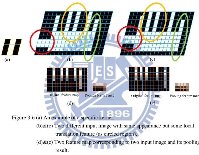
appeared in a larger patch. There is a simple example at Figure 3.6. Even though the input image
has the same appearance with translation, we can consider them to be the same appearance.
This is an advantage that neural network might not have.
Figure 3-6 (a) An example of a specific kernel.
(b)&(c) Two different input image with same appearance but some local translation feature (as circled region).
(d)&(e) Two feature map corresponding to two input image and its pooling result.
For the pooling layer, the feature map size will be down-sample from M+1) by
(N-M+1) to ((N-(N-M+1)/scaling factor) by ((N-(N-M+1)/scaling factor). We usually choose the factor
of (N-M+1) to get the down-sampled feature map with integer size.
Fully-connected layer
In the last layer, we will arrange all feature map to an one column feature. In addition, we
might have a target layer to do the final classification. All nodes in the feature column will
3.2.1.2 Learning algorithm of Convolutional Neural Network
Convolutional neural network use the same learning algorithm as traditional neural
network, which is back-propagation algorithm. The main concept of back-propagation is
minimize the error function of the training model. We can modify the weight in each layer to
get lower and lower error score. Gradient descent is the optimization method we use in the
learning algorithm. [14] might discuss all the derivation and implementation of convolutional
neural network in detail.
The error function of convolutional neural network is as equation (3-1). N means the total
number of input image in the training data set. C means the output target has C classes. 𝑡𝑘𝑛 is the target of kth image in nth class is 0 or 1. 𝑦𝑘𝑛 is the calculation result of kth image in nth class. Consider with respect to a single training data, the error function can be seen as equation
(3-2). 𝐸𝑟𝑟𝑜𝑟𝑁 =1 2∑ ∑ (𝑡𝑘 𝑛− 𝑦 𝑘𝑛)2 𝐶 𝑘=1 𝑁 𝑛=1 , (3-1) 𝐸𝑟𝑟𝑜𝑟𝑛 = 1 2∑ (𝑡𝑘 𝑛− 𝑦 𝑘𝑛)2 𝐶 𝑘=1 , (3-2)
We have different function operator in different layer. Therefore, the parameter update in
each layer might be difference. We will introduce them all in the following.
Back-propagation in fully-connected layer
We define the function operator in the last layer to be as equation (3-3). 𝑥𝑙 denotes the current layer l output, as last layer been layer L , input layer been layer 1. 𝑓(. ) is the activation function we choose. 𝑊𝑙 is the weight and 𝑏𝑙 is the bias in layer l.
𝜕𝐸 𝜕𝑊 = 𝜕𝐸 𝜕𝑎 𝜕𝑎 𝜕𝑊= 𝑥 𝑙−1(𝛿𝑙)𝑇, 𝑤𝑖𝑡ℎ 𝛿𝑙= (𝑊𝑙+1)𝑇𝛿𝑙+1⨀𝑓′(𝑎𝑙), (3-4)
where ⨀ denotes element-wise multiplication operator.
𝜕𝐸 𝜕𝑏 = 𝜕𝐸 𝜕𝑎 𝜕𝑎 𝜕𝑏= 𝛿𝑙. (3-5)
Back-propagation in pooling layer
The pooling layer produce a down-sampled feature maps. The function operator in
convolution layer is defined in equation (3-6).
𝑥𝑗𝑙 = 𝑓(𝑎𝑙) , 𝑤𝑖𝑡ℎ 𝑎𝑙= 𝛽
𝑗𝑙∙ 𝑑𝑜𝑤𝑛(𝑥𝑖𝑙−1) + 𝑏𝑗𝑙, (3-6)
where 𝑑𝑜𝑤𝑛(. ) represents a non-overlapped sub-sampling function. Each output map might have its own multiplicative biasβ and an additive bias b.
We need to update both multiplicative biasβ and additive bias b in this layer. The gradient
can be compute as fully-connected layer.
𝜕𝐸 𝜕𝑏𝑗 = ∑ (𝛿𝑗 𝑙) 𝑢𝑣 , 𝑤𝑖𝑡ℎ 𝛿𝑗𝑙 = 𝑓′(𝑎𝑙)⨀(𝑘𝑗𝑙+1∗ 𝛿𝑗𝑙+1) 𝑢,𝑣 (3-7) 𝜕𝐸 𝜕𝛽𝑗= 𝜕𝐸 𝜕𝑎 𝜕𝑎 𝜕𝛽𝑗= ∑ (𝛿𝑗 𝑙⨀𝑑 𝑗𝑙)𝑢𝑣 , 𝑤𝑖𝑡ℎ 𝑑𝑗𝑙 = 𝑑𝑜𝑤𝑛(𝑥𝑖𝑙−1) 𝑢,𝑣 (3-8)
Back-propagation in convolution layer
The output feature map will combine several feature maps. The function operator in
convolution layer is defined as equation (3-9), where 𝑆𝑗 represents a subset of input maps, *
denotes convolution operator.
𝑥𝑗𝑙 = 𝑓(𝑎𝑙), 𝑤𝑖𝑡ℎ 𝑎𝑙 = ∑ 𝑥 𝑖𝑙−1
𝑖∈𝑆𝑗 ∗ 𝑘𝑖𝑗𝑙 + 𝑏𝑗𝑙 (3-9)
The gradient of current layer might be sum over the next layer’s gradient corresponding to
units that connected to the node of interest in the current layer. The update function of kernel
previous layer which multiplied element-wise by 𝑘𝑖𝑗𝑙 during convolution. 𝛽𝑗𝑙+1 denotes the next pooling layer parameter. 𝑢𝑝(. ) denotes an up-sampling operation.
𝜕𝐸 𝜕𝑘𝑖𝑗𝑙 = ∑ (𝛿𝑗 𝑙) 𝑢𝑣(𝑝𝑖𝑙−1)𝑢𝑣 , 𝑤𝑖𝑡ℎ 𝛿𝑗𝑙 = 𝛽𝑗𝑙+1(𝑓′(𝑎𝑙) ⊙ 𝑢𝑝(𝛿𝑗𝑙+1)) 𝑢,𝑣 (3-10) 𝜕𝐸 𝜕𝑏𝑗= ∑ (𝛿𝑗 𝑙) 𝑢𝑣 𝑢,𝑣 (3-11)
3.2.2 Deep Neural Network
The reason we introduce “deep” neural network, not traditional neural network, is the high complexity of training data set. While the object we want to distinguish being more variability,
we need more hidden nodes and more layers to learn the model. However, traditional learning
algorithm is not efficiency for deep neural network architecture. For example, when we use
back-propagation algorithm to update our learning weight, we have the gradient from later layer
propagate to previous layer. The gradient might be tiny as propagating to the front layer. This
causes the weight update stagnant at local optima. Furthermore, the traditional learning
algorithm require labels to calculate error function and get gradient of weight to update the
model. The back-propagation algorithm find the relationship between input feature and output
target instead of finding the internal structure in training data set. Deep neural network is an
unsupervised learning method which learns the model without target. We can find the exist
structure behind the input data set.
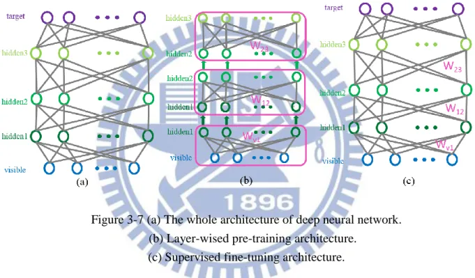
Hinton introduced a new learning method to train the model layer-by-layer instead of
learning the whole deep architecture once [5]. This algorithm has two stage : unsupervised
pre-training and supervised fine-tuning. At first, they take the whole deep architecture apart to train
deep neural network. Figure 3-7(b) shows the layer-wise pre-training architecture. After that,
we can get the initial weight of every layer and do supervised fine-tuning to get the relationship
between input image and output target by updating the weight slightly, shows in Figure 3-7(c).
We will introduce the structure of Restricted Boltzmann Machine (RBM) which is suitable for
binary visible and Gaussian Restricted Boltzmann Machine which is suitable for real-valued
visible both in section 3.2.2.1. In section 3.2.2.2, we will describe the learning algorithm of
pre-training and fine-tuning in detail.
Figure 3-7 (a) The whole architecture of deep neural network. (b) Layer-wised pre-training architecture.
(c) Supervised fine-tuning architecture.
3.2.2.1 Restricted Boltzmann Machine
Restricted Boltzmann Machine is a two layer and undirected model without intra-layer
connections. The bottom layer called visible layer is a set of binary units v ∈ {0,1} and the top layer called hidden layer is a set of binary units h ∈ {0,1}. We will use Gaussian Restricted Boltzmann Machine if the bottom layer is a set of real-valued units v ∈ [0,1] which we will describe later. The structure of RBM is shown in Figure 3-6(b) pink circled.
RBM is an energy-based model, the energy of a pair of (v,h) is defined in equation (3-12),
weights connecting hidden and visible units. The probability distribution of the pair of (v,h) is
defined in equation (3-13), where the constant Z is the normalization term.
Energy(v, h) = −𝑏𝑇𝑣 − 𝑐𝑇ℎ − 𝑣𝑇𝑊ℎ (3-12)
P(v, h) =𝑍1(𝑒−𝐸𝑛𝑒𝑟𝑔𝑦(𝑣,ℎ)) (3-13)
Since there is no connection within hidden layer and within visible layer, and the hidden
layer and visible layer are conditionally independent given one-another. Using these two
property, we can get the conditional distribution for each layer as equation (3-14) and (3-15),
where 𝑠𝑖𝑔𝑚(𝑥) =(1+𝑒1−𝑥) is a sigmoid function and M , N denotes the number units in visible layer and hidden layer Respectively.
P(h|v) = ∏ 𝑃(ℎ𝑁 𝑗 = 1|𝑣)
𝑗 , 𝑤𝑖𝑡ℎ 𝑃(ℎ𝑗 = 1|𝑣) = 𝑠𝑖𝑔𝑚(𝑐𝑗+ 𝑊𝑗𝑣) (3-14)
P(v|h) = ∏ (𝑣𝑀 𝑖 = 1|ℎ)
𝑖 , 𝑤𝑖𝑡ℎ 𝑃(𝑣𝑖 = 1|ℎ) = 𝑠𝑖𝑔𝑚(𝑏𝑖 + 𝑊𝑖ℎ) (3-15)
As mentioned previously, we use Gaussian Restricted Boltzmann Machine for real-valued
visible. The energy function and the conditional distribution is defined as equation (3-16) to
equation (3-18). Energy(v, h) = − ∑ (𝑣𝑖−𝑏𝑖)2 2𝜎𝑖2 𝑀 𝑖 − ∑ 𝑐𝑁𝑗 𝑗ℎ𝑗− ∑ ∑𝑖𝑀 𝑁𝑗 𝜎𝑣𝑖𝑖𝑊𝑖𝑗ℎ𝑗 (3-16) P(h|v) = ∏ (ℎ𝑀𝑗 𝑗 = 1|𝑣), 𝑤𝑖𝑡ℎ 𝑃(ℎ𝑗 = 1|𝑣) = 𝑠𝑖𝑔𝑚(𝑐𝑗+ ∑ 𝜎𝑣𝑖 𝑖𝑊𝑖𝑗 𝑁 𝑖 ) (3-17) P(v|h) = ∏ 𝑃(𝑣𝑁 𝑗 = 1|ℎ) 𝑖 , 𝑤𝑖𝑡ℎ 𝑃(𝑣𝑗 = 1|ℎ) = 𝑁𝑜𝑟𝑚𝑎𝑙(𝑣𝑖|𝑏𝑖 + 𝜎𝑖∑ ℎ𝑀𝑗 𝑗𝑊𝑖𝑗) (3-18)
3.2.2.2 Learning algorithm of Deep Neural Network
Unsupervised pre-training
We want to minimize the energy function of the RBM, on the other hand, we want to
maximize the log-likelihood given a training data v with model parameters θ. By using gradient
ascent method, we can get the learning rule for the model parameters. The first term of equation
(3-20) denotes the data-term which takes expectation over the training data set empirical
distribution P(h|v). The second term denotes the model-term which takes expectation over the
model distribution P(v,h). lnP(v|θ) = ln1𝑍∑ 𝑒−𝐸𝑛𝑒𝑟𝑔𝑦(𝑣,ℎ) ℎ = ln ∑ 𝑒ℎ −𝐸𝑛𝑒𝑟𝑔𝑦(𝑣,ℎ)− ln ∑𝑣,ℎ𝑒−𝐸𝑛𝑒𝑟𝑔𝑦(𝑣,ℎ) (3-19) 𝜕 𝜕𝜃lnP(v|θ) = − ∑ 𝑃(ℎ|𝑣) 𝜕 𝜕𝜃𝐸𝑛𝑒𝑟𝑔𝑦(𝑣, ℎ) ℎ + ∑𝑣,ℎ𝑃(ℎ, 𝑣)𝜕𝜃𝜕 𝐸𝑛𝑒𝑟𝑔𝑦(𝑣, ℎ) (3-20) ∆W = ϵ(𝐸𝑑𝑎𝑡𝑎[vℎ𝑇] − 𝐸 𝑚𝑜𝑑𝑒𝑙[vℎ𝑇]) , 𝑤𝑖𝑡ℎ 𝜖 𝑖𝑠 𝑡ℎ𝑒 𝑙𝑒𝑎𝑟𝑛𝑖𝑛𝑔 𝑟𝑎𝑡𝑒 (3-21) ∆b = ϵ(𝐸𝑑𝑎𝑡𝑎[v] − 𝐸𝑚𝑜𝑑𝑒𝑙[v]), 𝑤𝑖𝑡ℎ 𝜖 𝑖𝑠 𝑡ℎ𝑒 𝑙𝑒𝑎𝑟𝑛𝑖𝑛𝑔 𝑟𝑎𝑡𝑒 (3-22) ∆c = ϵ(𝐸𝑑𝑎𝑡𝑎[h] − 𝐸𝑚𝑜𝑑𝑒𝑙[h]), 𝑤𝑖𝑡ℎ 𝜖 𝑖𝑠 𝑡ℎ𝑒 𝑙𝑒𝑎𝑟𝑛𝑖𝑛𝑔 𝑟𝑎𝑡𝑒 (3-23) We use Gibbs sampling to approximate the model-term because of its difficulty. According
to the Markov chain Monte Carlo (MCMC) algorithm, we can sample the hidden nodes by the
visible nodes then sample the reconstruct visible nodes by the sampled hidden nodes. We will
do this procedure until the Markov chain converge in order to get the model-term. The
architecture of MCMC with Gibbs sampling is shown in Figure 3-8(a). However, it is not
efficient to run a MCMC to converge in an update step. In [5], Hinton propose a fast algorithm
which is called Contrastive Divergence. This method shows that the effect of sampling until the
Markov chain converge and sampling once might get close result. Therefore, the update
function can be approximated as equation (3-24) to equation (3-26). Figure 3-8(b) shows the
architecture of Contrastive Divergence algorithm.
∆W = ϵ(𝐸𝑑𝑎𝑡𝑎[vℎ𝑇] − 𝐸𝑟𝑒𝑐𝑜𝑛𝑠𝑡𝑟𝑢𝑐𝑡[vℎ𝑇]) , 𝑤𝑖𝑡ℎ 𝜖 𝑖𝑠 𝑡ℎ𝑒 𝑙𝑒𝑎𝑟𝑛𝑖𝑛𝑔 𝑟𝑎𝑡𝑒 (3-21)
∆c = ϵ(𝐸𝑑𝑎𝑡𝑎[h] − 𝐸𝑟𝑒𝑐𝑜𝑛𝑠𝑡𝑟𝑢𝑐𝑡[h]), 𝑤𝑖𝑡ℎ 𝜖 𝑖𝑠 𝑡ℎ𝑒 𝑙𝑒𝑎𝑟𝑛𝑖𝑛𝑔 𝑟𝑎𝑡𝑒 (3-23)
Figure 3-8 (a) Architecture of MCMC by using Gibbs sampling. (b) Architecture of Contrastive Divergence algorithm
We will train the RBM layer-wise staring from visible layer and hidden layer one. When
we get the weight W1 between visible layer v and hidden layer one h1, we treat the real-valued
probabilities of the conditional distribution E[P(ℎ1|v; 𝑊1)] as the visible units in the second RBM and so on. After we get all trained weight between layers, we can do the next stage,
supervised fine-tuning.
Supervised fine-tuning
We learned the internal structure of the training data set in the previous stage. Next, we
want to learn the relationship between input training data set and the output targets for
classifying the different class in the training data set. We use the back-propagation algorithm to
learn the overall optimization solution.
3.3 Applicable to Hand Gesture Recognition
As we mentioned before, the hand has extremely distinct shape and appearance from
different gestures. Using traditional convolutional neural network or traditional deep neural
In order to improve the accuracy in the video testing, we add some tracking technique described
in Section 3.3.3.
3.3.1 Feature Extraction by Convolutional Neural Network
We want to use convolutional neural network to learn the feature from training data set
directly. Traditional convolutional neural network have the features for single kernel size and it
is restricted to be square and the down-sampling scaling factor for feature map’s width and
height are limited to be the same. As we observe the training data set of the hand gestures, we
find that hands can be composed of fingers and a palm. Fingers are different orientation,
different length, long and narrow strip. Palm is a larger rectangle which width and height ratio
is extremely different from the fingers. Furthermore, the four hand gestures we need to classify
are composed of different number of fingers and the open or close palm. Therefore, the features
we want to learn in the hand gesture training data set might be modify to some long and narrow
strips and some rectangles close to square. In order to cope with the different kernel size for
width and height, we also modify the down-sampling scaling factor could be distinct for the
width and height. Also, we want to represent the hand gestures by more different kernel size to
get a more robust feature space of the hand gestures. Therefore, we need some algorithm to
choose better features of different kernel size and combine different kernel size feature to find
more robust feature space for hand gestures.
The convolutional neural network architecture we attempt is shown in Figure 3-4. We set
one convolution layer and one pooling layer to get the local features of the hand gesture images.
Also, we don’t use the last full-connected layer for the hand gesture classification. We only extract the feature vector from the output of the pooling layer. The pooling scaling factor might
be cope with the kernel size we choose at the convolution layer. We will have a summary of the
3.3.1.1 Non-square kernel size and pooling scaling factor
The important issue at convolutional neural network learning is the choice of kernel size.
If the kernel size might be square, a larger square or a smaller square is not the best choice. As
using the smaller one, it will turn on some position of the feature map because of the clutter
background, which is shown in Figure 3-9 (a). The blue rectangles are the clutter background
features we don’t need and red rectangles are the hand features we want. In Figure 3-9(b), we
can discover that a larger block might get a complex feature to cope with the multiple fingers.
However, if we have a complex feature, it might not represent the hand gestures good for the
different hand gestures. Different number of fingers in the patch and the close or open palm
might need different features to represent. These will reduce the effect we want to have in the
learning feature stage of convolutional neural network. We want to learn the local features of
the hand gestures not the global features in the whole image. For a specific long and narrow
block, we can represent the fingers more efficient, as shown in Figure 3-9(c).
Figure 3-9 (a) The kernel of convolutional neural network is a small square. (b) The kernel of convolutional neural network is a large square. (c) The kernel of convolutional neural network is a long and narrow stipe.
we have different viewpoints of the hand gestures, we not only need long and narrow rectangles
but also need short and wide rectangles for different orientation fingers. However, convolutional
neural network could not tolerate the different kernel size learning at once, we need to train the
different kernel size feature one by one. Figure 3-10 shows four different kernel size features
for the hand gesture training data set. The kernel size are 3*3, 6*6, 7*3, 3*7 pixel by pixel in
Figure 3-10(a) to (d). Each row has sixteen features learned by the convolutional neural network.
Figure 3-10 (a) The convolutional neural network feature learned by 3*3 kernel size. (b) The convolutional neural network feature learned by 6*6 kernel size. (c) The convolutional neural network feature learned by 7*3 kernel size. (d) The convolutional neural network feature learned by 3*7 kernel size.
After the convolution layer, we have the pooling layer to down-sample the feature map we
get from previous layer. The pooling concept might let the convolutional neural network to be
translation invariance as we mention in Section 3.2.1. We calculate the mean of a local patch of
the feature map to indicate the feature is existence or not at a small region in the original input
image as shown in Figure 3-4. The pooling scaling factor is limited as the same for width and
height in the conventional convolutional neural network. We modify it to coordinate the long
and narrow rectangles and the short and wide rectangles of kernel we learned for the hand
gesture. Therefore, we can down-sample for different scaling factor for the feature map width
invariance. The corresponding scaling factor for four different kernel size is shown in Table
3-1. The unit for the kernel size and scaling factor are pixels.
1 2 3 4
Width Height Width Height Width Height Width Height Kernel Size 3 3 6 6 7 3 3 7 Scaling Factor 6 6 5 5 4 6 6 4
Table 3-1 Different kernel size correspond to different pooling scaling factor.
The feature maps of different kernel size we get from convolutional neural network after
pooling layer are shown in Figure 3-14(a) to (d). We random choose some example from
training data set to get the feature maps for the four different gestures, each gestures has five
example images. The top to down blocks are the stop gesture, pointer gesture, ok gesture and
wave gesture. We can figure out that a long and narrow kernel size, such as 3*7 and 7*3 might
be good at fingers feature, as the red circled region in Figure 3-11 (c) and (d). The small square
kernel size, 3*3 and 6*6, might get the rough contour of the hand gesture, as the red circled
Figure 3-11 (a) The feature map of kernel 3*3, red circled region show the rough contour of hand gestures.
(b) The feature map of kernel 6*6, red circled region show the rough contour of hand gestures.
(c) The feature map of kernel 7*3, red circled region show the finger feature. (d) The feature map of kernel 3*7, red circled region show the finger feature.
3.3.1.2 Combination of different kernel size feature
Because of the complex shape and extremely variant of appearance for the hand gestures,
the features might be different size, such as small square, large square and rectangles. Figure
3-10 shows some example for different kernel size for the hand gestures. Therefore, we want to
use different kernel size to express the hand gesture features as shown in Figure 3-12. For
vertical fingers, horizontal fingers, fist and palm, we need different kernel size to represent its
local feature. We design four different kernel size, 3*3, 6*6, 3*7 and 7*3. We will train sixteen
kernels for a specific kernel size, then choose four of them. The reason why we need to train
sixteen kernels then choose four of them rather than only train four kernels for one kernel size
is the overall kernel number. If we only set four kernels for the convolutional neural network
model, the model might learn more complex feature than we set sixteen kernels for it. It expect
use four features to represent the whole training data set. However, we have sixteen feature to
represent the training data set not four. The features we want to learn is the simple, local feature,
not the complex and global feature. Figure 3-13 shows the different between four features and
sixteen features for a convolutional neural network model. Figure 3-13(a) shows the features
we learned for sixteen kernels and choose four of them and the corresponding feature maps.
Figure 3-13(b) shows the features we learned for only four kernels and the corresponding
feature maps. We can figure out that for four specific kernel, we get a more complicated feature
maps. We couldn’t easily determine the gestures for ok and wave as shown in red rectangles of Figure 3-13(b).
As record in Table 3-1, we have four different convolutional neural network for four
different kernel size. For kernel 3*3, the feature map at the convolution layer is 48*48. After
the pooling layer, the down-sampled feature map is 8*8 because of the scaling factor is 6*6.
For kernel 6*6, the feature map at the convolution layer is 45*45. After the pooling layer, the
down-sampled feature map is 9*9 because of the scaling factor is 5*5. For kernel 7*3, the
feature map at the convolution layer is 44*48. After the pooling layer, the down-sampled feature
map is 11*8 because of the scaling factor is 4*6. For kernel 3*7, the feature map at the
convolution layer is 48*44. After the pooling layer, the down-sampled feature map is 8*11
because of the scaling factor is 6*4. We transform the feature map from two dimension to one
dimension vector and concatenate four different kernel size to get our overall feature vector.
The feature vector dimension is 1284. (((8*8)*4) + ((9*9)*4) + ((11*8)*4) + ((8*11)*4) = 1284)
As we have sixteen features for a specific kernel size and four different kernel size, we
need some algorithm to choose the best combination for different kernel size. We take an
intuitive idea to solve it. The criteria we choose are the more far from different gestures and
more close for same gestures in the feature space. The concept is shown in Figure 3-14. Figure
3-14(a) shows the feature space we prefer to and Figure 3-14(b) shows the feature space which
the gestures is not easy to separate. We random sample four of sixteen features for a specific
kernel size and combine four different kernel size to get a feature vector with different kernel
size. Then calculate the difference map in different gestures of the specific kernel. Also, we
calculate the difference map in same gesture of the specific kernel. After we get the difference
map, we calculate the variance of the map and compute the ratio of the variance for same
gestures and the variance for different gestures as equation (3-24). We choose the smallest value
of the ratio to get a feature space with large distance from the different gestures and close in the
same gestures. There are some examples in Figure 3-15.
Figure 3-14 (a) The schematic diagram of feature space which is easy to separate. (b) The schematic diagram of feature space which is not easy to separate.
Figure 3-15 The feature vectors combining different kernel size for the hand gestures.
3.3.2 Deep Convolutional Neural Network Classification
as mentioned before. Our training data set for deep neural network is shown in Figure 3-3. The
architecture of our deep neural network model is shown in Figure 3-17(a). Our feature vector
combines four different kernel size and each kernel size has four features. The input feature
dimension is 1284 and output target is 5(four gestures and background). The model with layers
of size 1284-1024-1024-1600-5. Also, we apply a sigmoid function after the hidden units and
a softmax function after the target units as the activation function, as shown in Figure 3-17(b).
Equation (3-25) and (3-26) are the formula of sigmoid function and softmax function
respectively.
sigmoid(x) =1+𝑒𝑥𝑝1 −𝑥 (3-25)
softmax(𝒙)𝑖 = ∑𝐾𝑒𝑥𝑝𝑒𝑥𝑝𝑥𝑖𝑥𝑘
𝑘=1 , for K is the dimension of 𝒙 (3-26)
Figure 3-16 (a) Our deep neural network model architecture.
(b) The example of the activation function after the hidden node.
The deep neural network training procedure is mentioned as Section 3.2.2. We have two
stages, that is, unsupervised pre-training stage and supervised fine-tuning. We trained the neural
divergence algorithm to update the weight between two layers. The basic concept for Restricted
Boltzmann Machine is to find the hidden nodes which can represent the visible nodes better. As
we use the hidden nodes to re-sample the visible nodes, we can figure out whether these hidden
nodes could represent these visible nodes or not by calculating the different between visible
nodes and the re-sampling visible nodes. After several times updating, we can get the hidden
nodes which can represent our visible nodes. We might get some combination for the input
features, on the other words, more global features be composed of the local features in the
visible layer. As we trained the first two layers of the model, we might use visible nodes and
the trained weight between visible nodes and hidden one nodes to get the output of hidden layer
one nodes. Then we do the second two layers training by setting the hidden one nodes as the
visible nodes, and so on. Finally, we have trained all the weights between any two layers. After
that, we stack the two layer-wise structure to be a deep neural network architecture. At the
supervised fine-tuning stage, we use the back-propagation algorithm to minimize the error
function by updating the weight we get from previous stage. We adjusted the weight slightly, to
get the best solution of this neural network model. At last, we could have a classifier for hand
gesture recognition by using the deep neural network model.
3.3.3 Tracking Technique
The purpose of an object tracker is to find the object position from previous frame to next
frame. The tracking method might get the trajectory of the object in every frame which we are
interested. In [15], according to different object representation, the tracking method can be
categorized into three types, point tracking, kernel tracking and silhouette tracking. Their
one might find the optimum solution of the silhouette or contour matching. Figure 3-17(a) to
(c) briefly illustrate the three tracking method. The dot arrow denote the previous motion
estimation and the dash arrows denote the predict motion for the next frame. The solid nodes
denote the previous hand gesture position and the light-colored nodes denote the predict hand
position. Because of the complex changes for the hand shape from different gestures, there isn’t
a robust tracking method for the hand gestures. Therefore, we only use the basic concept of the
tracking technique in our hand gesture recognition algorithm.
Figure 3-17 (a) The example of point tracking method. (b) The example of kernel tracking method. (c) The example of silhouette tracking method.
The idea of our tracking algorithm are the constraints of the searching region of our
detection algorithm and using a simple two dimension correlation of two patches to find the
similarity of them. Because of the video will have about thirty frames in a second, the hand
position won’t be distance from two successive frame. Also, the motion of previous two frame and next two frame won’t be a lot of difference. We restrict the searching region of our detection by using convolutional neural network and deep neural network. The searching region will
adjusted according to the motion estimation. For example, as we estimate the object move from
the bottom left corner to the top right corner, the range we search at the top right corner will
larger than the bottom left corner to cope with the object trajectory. We estimate the object
our hand gesture recognition result for the previous frames. Figure 3-18 shows an example of
searching region adjustment and the motion estimation for our proposed method. In Figure
3-18, the blue dash block is the adjustment of searching region for the detection algorithm and
the green arrow is our motion estimation result. For the similarity issue, we use the two
dimension correlation function for the target patch and a testing patch. The target patch is the
hand gesture we find in the previous frame whether getting by detection or by tracking. The
testing patches are the adjacent region of the target patch. The two dimension correlation
function is described in equation (3-27),
𝑐𝑜𝑟𝑟2 = ∑ ∑ (𝐴𝑖 𝑗 𝑖𝑗−𝐴̅)(𝐵𝑖𝑗−𝐵̅)
√∑ ∑ (𝐴𝑖 𝑗 𝑖𝑗−𝐴̅)2√∑ ∑ (𝐵𝑖 𝑗 𝑖𝑗−𝐵̅)2
, (3-27)
where A denotes the target patch and B denotes the testing patch. Aijis the pixel at the i row and
j column in the target patch and same as Bij. 𝐴̅ and 𝐵̅ are the mean of the target patch and
testing patch respectively. We have an example target patch and some testing patches to shown
the correlation between two patches in Figure 3-18.
Figure 3-19 The example of target patch and three testing patch with its two dimension correlation for the target patch.
In order to reinforce the hand position constraint, we use two maps, position map and
motion map to weighted the result of detection and tracking. The position map is obtained from
the previous hand gesture recognition result. We use a two dimension Gaussian distribution to
model the position map for the previous hand gesture recognition is one and drop to the
surrounding. Also, the motion map is obtained from the previous hand gesture recognition result
add the displacement we predict by motion estimation. The previous position add the
displacement is set to one and drop to the surrounding as a two dimension Gaussian distribution.
Figure 3-20 shows an example of the position map and motion map. The blue point and green
point in the position map are the previous hand gesture recognition result. The red arrows in the
Figure 3-20 The examples for the position map and the motion map.
3.4 Refinement
The last stage of our hand gesture recognition algorithm is refinement. We have to choose
the result from the detection algorithm and the tracking algorithm. The first refinement step is
the weighted score for both detection and tracking result. The weighted are the position map
and the motion map. The closer the local patch and the previous hand gesture recognition result
the higher weighted it has. After we get the weighted score for both detection and tracking result,
we will find the highest two scores to represent the right hand result and left hand result. Figure
3-21 is the flowchart of the weighted score for detection and tracking result. This step is
Figure 3-21 (a) The flowchart for the weight score of detection result. (b) The flowchart for the weight score of tracking result.
Secondly, we use the temporal information to improve the stability of our hand gesture
recognition results. The idea of our proposed refinement for temporal domain is the records of
seven frames to average the score for four different gestures. The closer to the frame we want
to figure out the hand gestures in the temporal domain, the higher weighted we multiply to the
score of detection or tracking result we choose. Figure 3-22 is an example for the temporal
information refinement in our proposed method. The rows under the arrow is the result of our
choice for the detection and tracking result in the temporal domain from ten frames before the
frame we are processing. The square above the arrow is the refinement result in the frame we
are processing. We can see that even the result in the processing from is distinct from previous
few frames, we can use the temporal information to correct the result. This information is under
the limitation of the hand shape would not dramatic change.