IEEE TRANSACTIONS ON COMPUTERS, VOL. 43, NO. 1, JANUARY 1994 87
Brief Contributions
On Distributed Computing Systems Reliability Analysis Under Program Execution Constraints Deng-Jyi Chen, Member, IEEE, and Min-Sheng Lin
Abstract-This correspondence presents an algorithm for computing the reliability of distributed computing systems (DCS). The algorithm, called the Fast Reliability Evaluation Algorithm, is based on the factoring theorem employing several reliability preserving reduction techniques. The effect of file distributions, program distributions, and various topolo- gies on reliability of the DCS is studied in detail using the proposed algorithm. Compared with existing algorithms on various network topolo- gies, file distributions, and program distributions, the proposed algorithm is much more economical in both time and space. To compute the distributed program reliability, the ARPA network is studied to illustrate the feasibility of the proposed algorithm.
Index Terms-Distributed program, distributed system, factoring the- orem, graph theory, reliability, reliability-preserving reduction, spanning tree.
I. INTRODUCTION
Recently, the distributed computing system (DCS) has become increasingly popular because it offers higher fault tolerance, potential for parallel processing, and better reliability in comparison with other processing systems [1]-[5]. A typical DCS consists of processing elements (PE’s), memory units, data files, and programs as its resources. These resources are interconnected via a communication network that dictates how information could flow between PE’s. Programs residing on some PE’s can run using data files at other PE’s as well. For successful execution of a program, it is essential that the PE containing the program and other PE’s that have the required data files, and communication links between them must be operational. Using this concept, distributed program reliability (DPR) is defined as the probability of successful execution of a distributed program that runs on some PE’s and needs to communicate with other processing elements for remote files. Distributed system reliability (DSR) is defined as the probability that all programs with distributed files can run successfully despite some faults occurring in the PE’s and/or in the communication links [6].
In [6], a minimum file spanning tree (MFST) is proposed to represent the multiterminal connection required for executing a distributed program, and a two-pass method for the reliability analysis of DCS is developed. In this method, all MFST’s are obtained by using the breadth-search method. After finding the MFST’s, since they are not disjoint with each other, the algorithm requires other reliability evaluation algorithms such as SYREL [ 121 to generate the reliability expression. Although the method is elegant, it does generate a lot of replicated trees during the processing and thus will be inefficient. Instead of generating MFST’s, one algorithm, called Manuscript received March 7, 1991; revised November 15, 1991. This work was supported in part by the National Science Council under Contract NSC- 80-0408-E009-16 and in part by the Chung San Institute of Technology under Contract 7S79-0210-D009-03.
The authors are with the Institute of Computer Science and Information Engineering, National Chiao-Tung University, Hsin Chu, Taiwan, Republic of China.
IEEE Log Number 9204158.
FARE, has been proposed in [13] and [14] to compute DPR directly by using a connection matrix. Based on the assumption that the PE’s (nodes) in the DCS are perfect, it does not require additional reliability evaluation algorithms to convert a multiterminal connection into a reliability expression. The shortcoming of this algorithm is that it is not applicable for distributed programs running on more than one node.
In this correspondence, we propose a new algorithm called the Fast Reliability Evaluation Algorithm (FREA) that employs a differeht concept to compute the reliability of DSR and DPR. It is based on the generalized factoring theorem with several reliability preserving reductions to reduce the computation tree. The factoring theorem for the exact computation of li-terminal reliability in undirected networks has been proposed since 1958 by Moskowitz [15]. Recently, several papers have addressed worst case computational complexity and the optimality of classed factoring algorithms and related algo- rithms, for example, Ball [16], Chang [17], Satyanarayana and Chang [ 181, and Wood [ 191 to name a few. Unlike the I<-terminal reliability problem, where li-terminal nodes are fixed and given, the distributed program reliability problem does not have fixed Zi -terminal nodes. The li-terminal nodes in the distributed program reliability analysis can be changed dynamically due to the effects of link or node failure, using data files and programs distribution, and the topology of the network. Therefore, we may say the network reliability problem is considered to be static-oriented, whereas the distributed program re- liability problem is dynamic-oriented. Naturally, distributed program reliability problems are considerd to be more complex and difficult than computer network reliability problems.
11. NOTATIONS AND DEFINITIONS
Notations and definitions used in the rest of correspondence are summarized here.
FST
MFST
0018-9340/94$04.00 0 1994 IEEE
Undirected DSC graph in which the set of vertices (nodes) in 1 ~ represents the PE’s and the links (edges)
in E represent the communication links. Node representing a processing element i . Link between processing elements i and j. G with a node ss. called starting node, indicates where the FREA algorithm begins to generate sub- graphs.
Probability that link .rl Data file I .
Distributed program i .
Set of programs that can be run at processing element .r , .
Set of data files available at processing element 2,. Set of data files needed to execute P,.
Set of programs to be executed.
Set of data files needed to execute all programs in
P S (i.e., F S = U P , E P \ FA’Vt).
Spanning tree that connects the root node (the pro- cessing element that runs the program under consid- eration) to other nodes, such that its vertices hold all the needed files for the program under consideration. An FST such that there exists no other FST that is a subset of it.
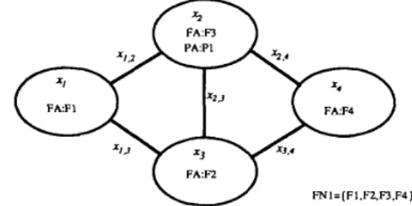
88 IEEE TRANSACTIONS ON COMPUTERS, VOL. 43, NO. 1, JANUARY 1994 FA:FI.F4 P A R x2.3 FAF1 FNI=(FI.F2.F3.F4]
Fig. 1. Simple distributed computing system. Fig. 2. Simple distributed computing system with different file distribution.
G - x 2 , 3 G CE
Graph G with edge x,,, deleted.
Graph G with edge x 2 , , contracted such that nodes z, and x, are merged into a single node. This new merge node contains all data files and programs that were in nodes z1 and 1,.
Reliability of the DCS graph G.
R ( G )
Since trees and subgraphs are used to represent the intermediate communication structure of the DCS, they are used interchangeably in the rest of this correspondence.
111. DISTRIBUTED PROGRAM RELIA~ILITY ANALYSIS Considering the distributed computing system in Fig. 1, there are four processing elements ( I I , Z Z , 2 3 , ~ 4 connected by links ) ~ 1 , ~ , ~ 1 , 3 , ~ 2 , 3 , ~ ~ , 4 , and 2 3 4 . Processing element xl contains two data files ( F I and F z ) and can run PI directly from here to
communicate with other nodes for accessing data files required to complete the execution of P I . Detailed information for each node is
summarized in FA,, P A , , and F N , ( 3 = 1,.
.
. ,4) in Fig. I . Let program PI require F1, F z , and F 3 to complete its execution in the DCS. Also, PI can be run on both nodes 1 1 and z 4 in the DCS (Fig. I). We can identify some file spanning trees (FST’s) rooted on X I from the DCS graph:Z 1 2 2 1 3 2 1 , 3 2 2 , 3 , 5 ) x i 1 3 Z q z 1 , 3 1 3 . 4 , 6) x i k z ~ 3 ~ 4 x i , z ~ z , 3 ~ 3 4 , 7)
2 1 2 ~ 2 3 2 4 % i , z 2 ~ , 4 1 3 , 4 , 8) 2 : 1 1 ~ 2 3 ~ z i , 3 x z , 3 x z 4 , and 9) Z I Z Z Z ~ ~ ~ X I , 3 x 3 , 4 x2,4.
If PI can be run only on node X I , the MFST’s are 1) ~ 1 ~ 2 ~ 1 . 2 , 4) x 1 2 2 1 3 2 1 , 3 2 2 , 3 , and 5 ) 2 1 1 3 1 4 2 1 , 3 2 3 , 4 .
If we also consider the FST rooted on z 4 . then the MFST’s for PI are 1) 2 1 2 2 2 1 , 2 . 4) 2 1 1 2 2 3 z 1 , 3 1 2 , 3 . *) 1 3 x 4 1 3 4 , and *) 1 2 2 3 3 4 X 2 , 3 2 2 , 4 . The last two MFST’s marked by
*
are rooted on node z4 instead of zl.Since the MFST’s connect the root node (the PE that runs the program under consideration) to some other nodes such that its nodes hold all the needed files for the program under execution, the DPR can then be determined by computing the probability that at least one of these MFST’s is working. Thus the distributed program reliability for a given program j can be defined as the probability that at least one MFST of program j is working [6]. The DPR measures the reliability of a particular distributed program. For the entire DCS to be operational, several such programs or a given set of distributed programs must be operational. A system-level reliability measure for all distributed programs to be operational is defined in [6] as the probability that at least one MFST of all distributed programs is working.
For computing the reliability of the entire DCS, the concept of MFST has been extended to the minimal file spanning forest (MFSF) [14]. Based on the concepts of the MFST and MFSF, Kumar and his colleagues developed algorithms to generate all MFST’s [6]
1) z l Z Z z 1 , Z r 2) x 1 2 2 z 3 T I 2 x 2 3 . 3 ) z 1 1 2 z 4 1 1 , 2 2 Z , 4 7 4)
and MFSF’s [20], respectively. Once the MFST’s and MFSF’s are obtained, SYREL [12] is called for evaluating the reliability.
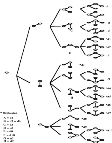
Although the concept of their algorithm is very straightforward, it generates many replicated trees during the MFST generating process. Considering the DCS in Fig. 2, for finding all the M F S P s for P I , let us use Kumar’s algorithm [6] to generate the MFST’s. The algorithm starts from finding the MFST’s of size 0, and then size 1,
. . .
until sizen - 1. As we can see in Fig. 3, the replicated trees (e.g., trees B, d2, and d4 are replicated) have been generated by their algorithm. Thus a procedure, called CLEAN, is required to remove these replicated trees.
Because the MFST’s generated by the algorithm in [6] are not disjoint with each other, other reliability computation programs such as SYREL [ 121 are required to generate the reliability expression. For the node perfect case, one algorithm, called FARE, which can evaluate DPR in one pass, is reported in [13]. Since a matrix is used to represent the subgraphs in the FARE algorithm, the reliability analysis methods cannot be used to evaluate the reliability of a program running on more than one node.
IV. DERIVATION OF FREA ALGORITHM
In this section, we present a new algorithm, called FREA, for the reliability evaluation of DCS. The FREA algorithm is based on the generalized factoring theorem employing several reliability preserving reductions to reduce the size of computed graphs and to simplify the reliability computation. To illustrate our approach, we begin by presenting the concept of a generalized factoring theorem and then several reliability preserving reductions.
A. Generalized Factoring Theorem for Distributed
Program Reliability
The factoring theorem of network reliability [18] is the basis for a class of algorithms for computing h--terminal reliability. This theorem establishes the validity of the following conditional reliability formula:
R(G) = p,,,R(G g? zt,,)
+
qt,,R(G - ~ t , j ) . (1)The theorem can be used to interpret topologically the following conditional reliability formula for a general binary system S with components I * ,, :
R ( S ) = P,,,R(SIG,, works)
+
q Z , , R ( S l ~ , , , fails). (2) Thus, (1) can be generalized in the following manner. Suppose that nodez, isthestartingnodeofgraphG,, a n d x , , l , z , , 2 , . . . , andxs,k are the edges incident on xs. We can obtain the following generalized equation:IEEE TRANSACTIONS ON COMPUTERS, VOL. 43, NO. 1, JANUARY 1994 89 * Replicated A = d l B = d2 = d4 C = d3 D = d 5 E = d8 F = d10 G = d7 H = d9
e
Fig. 3. Generation of replicated trees in MFST [61 algorithm
+
qs,1qs,2. . .
q s , k - l p s , k R ( G - 5 s 1 - x s , 2Z s , k - l @ z s , k )
- . . . _
+
q s , 1 q s , 2 . . . q ~ , k R ( G - x ~ , l - x ~ , ~ - . . . - x s , k ) . (3) Equation (3) is obviously true. For the proof of its correctness, readers are referred to [21]. Equation (3) can be recursively applied to the induced graph until either 1) the further induced graph with node zs containing all needed data files and all programs to be executed, or 2) the further induced graph with no FST’s is obtained. The induced graph of the former case represents a success, wheres the latter case represents a failure. It is easy to see that subtrees (or subgraphs) generation based on (3) will be completely disjoint. Since all of these disjoint terms represent either a success or a failure, one can simply sum all these disjoint terms together to produce the reliability expression of the system. Thus, the dominant factor for the reliability computation becomes the subgraph generation which is the process to produce these disjoint terms. Since the subgraph generation based on (3) will be completely disjoint, it guarantees no replicated trees will be generated during the expansion of the tree. This is one of the key reasons why the FREA algorithm will generate less subgraphs than existing algorithms. The other major reason will be the use of several reliability preserving reduction techniques, which will be discussed in the following section, to reduce the size of the graph.B. Reliability Preserving Reductions for the DCS Reliability Evaluation
To reduce the size of graph G and, therefore, reduce the state space of the associated reliability problem, reliability preserving reductions
can be applied. Some reductions are designed and developed to speed up the reliability evaluation.
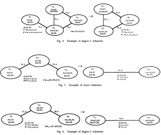
Definition I: Degree-1 Reduction Degree-1 reduction is to re- move nodes and their incident edges that contain no needed data files and programs under consideration. Considering the DCS in Fig.
4 for computing DPR1, since node x1 does not contain PI and any
needed data files (F1, F2. and F3), the degree-1 reduction is applied
to remove node ~1 and its incident edge s1 3 . The resulting graph is also shown in Fig. 4.
Definition 2: Irrelevant Component Deletion Let Go = ( V o , E o )
be a connected component of G, and it is not connected to the rest of the components of G. If there are no FST’s in Go then the component
Go is irrelevant and a reduction is applied to delete component Go. Definition 3: Parallel Reduction Let x ,
,
and xi,
be two parallel edges in G. Then, G’ is obtained by replacing x , , ~ and xi,, with a single edge X , (or p t , j = p , + p : , , - p : , , p : , J ) . The parallel reduction for DPR and DSR problems is the same as the parallel reduction for the h--terminal network reliability problem.Definition 4: Series Reduction There are some differences in se-
ries reduction between the DCS reliability problem and the K -
terminal network reliability problem. The series reduction for the Zi-terminal network reliability problem is defined in [19] and is recalled here.
Let z t , 3 and x t k be two series edges in G such that degree (z,) = 2 and xI $!
K.
Then, G’ is obtained by replacing x ~and , ~x , , k with a single edge X , , k such that p, k = p:,kp,,,.
The series reduction for the DCS reliability problem is the same such that p ,
,
= 1 - qt*3qiIEEE
n
.F3 1
I -. . ._ .
__
TRANSACTIONS ON COMPUTERS, VOL. 43, NO. 1, JANUARY 1994
Fig. 4. Example of degree-1 reduction.
Fig. 5. Example of series reduction.
Fig. 6. Example of degree-2 reduction.
as the preceding description except that the condition of st li is replaced by F A ,
n
F N =0
and P A ,n
PN =0.
In other words, if degree ( x t ) = 2 and node spz contain no needed data files and programs to be executed, then we apply the series reduction on G.For example, Fig. 5 presents a case of series reduction for computing For the case of degree (s2) = 2 and node xt contains some needed data files or programs to be executed, the series reduction may be performed. The details of this case will be described later in the degree-2 reduction.
Definition 5: Reducible Node A node x z is called a reducible node for distributed program Pj in graph G if and only i f 1) the degree of node x1 is two in graph G, and 2) the degree of node z t in the MFST’s of P, that contains node xt must also be two.
Theorem 1: Node x z is a reducible node for distributed program
P, if it satisfies the following conditions: a) Node degree is two, and
b) FA,
2
( F A ,n
FN) and PA,2
( P A , n P N ) and FAk2
( F A , f l F N ) and PAk
_>
(Pd, f lPLY)
(where node SI, andx, are the two adjacent nodes of x r ) .
Proof: Case 1 : Some MFSTt generated for DPR, contain node
s t . Suppose sz satisfies the properties of Theorem 1 and z t is not a reducible node, then it implies either i) s,’s node degree is not two, or ii) xz’s node degree in the MFST is not two according to the definition of a reducible node. In the former case, that z2’s node degree is not two is violated in the first given property in Theorem DPRi
.
1 that declares the degree of node x t is two (since we assume x t satisfies the properties of Theorem 1). Thus, it must be the latter case, that is, s t ’ s node degree in the MFSTt is not two. Since the first given property in Theorem 1 states that the degree of node x t is two, the MFSTt that contains node s, can only have the degree of node z1 less than or equal to two. Furthermore, in the latter case, we assume that the degree of node sz in the MFST is not two; then it must be one. This implies that node s, is a leaf node in the MFSTt
.
Based on the second given property in Theorem 1, it implies that node st contains a subset of needed data files in node sj or X k and a subset of programs to be executed in node .rl or S I , . From these facts, we conclude that x z is one of the nodes in MFSTt is incorrect. In other words, MFSTt is not a minimal file spanning tree. Thus, the assumption that node s, is not a reducible node is not true. Therefore, node .rt must be a reducible node.Case 2: No MFST’s contain node x , . Theorem 1 is obviously true
for this case.
Using Theorem 2, it is easy to verify the following corollary.
Corollury 1: If a node s, satisfies the following properties: 1) the degree is two, and 2) F A , f l F S = 0 and P A , f l PiV =
0,
then node .r2 is a reducible node.Definition 6: Degree-2 Reduction Suppose node s, is a reducible node, then one can apply series reduction on node sz and move data files and programs within node s, to one of its adjacent nodes x J or Sk. This reduction case is called degree-2 reduction. Fig. 6 presents an example of such reduction.
IEEE TRANSACTIONS ON COMPUTERS, VOL. 43, NO. 1 , JANUARY 1994 91
PA:Fl.FZ
FNl-{Fl.PZ.F3.F4) MPSTflI):
Fig. 8. Basic node structure of trace tree.
....
....
@' GO'
Fig. 7. Example of DCS and all MFST's for program 1 under consideration.
To prove degree-2 reduction is correct for DPR analysis is trivial; readers are referred to [21]. In fact, the series reduction is just a special case of degree-2 reduction that meets the properties of Corollary 1.
No C. Identification of Reducible Nodes
In this subsection, we propose an algorithm to identify all reducible nodes in a DCS graph.
Let us consider the DCS shown in Fig. 7. Although s 1 and S I are reducible nodes by the definition of the reducible node, only xq can
be identified based on Corollary 1. Thus, the problem is how to find all the reducible nodes in the DCS graph. The most straightforward solution is to find all the MFST's, and then to validate the nodes of those MFST's that contain the reducible nodes. However, such a solution inherits the problem in Kumar et ai. [6], which will generate
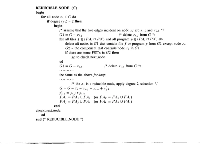
several replicated trees and therefore is not a good approach. In the following, we present a new algorithm, called RE- DUCIBLE-NODE, to identify all the reducible nodes without the generation of all MFST's. The basic concept of the algorithm can be explained from the following statements.
Let G be the original graph that contains node s I with node degree = 2. Edges s t , and s, k are the two incident edges on s t . Suppose node .r, is not a reducible node, then it must be a leaf node of some MFSTt (also discussed in the proof of Theorem 2 ) . Thus, node .rz
must contain some needed data files or programs to be executed that are not resident at other nodes in the same MFSTt.
To test which data file causes the node
I ,
that becomes a leaf node of the MFSTt, we can repeatedly check each needed data file, Fa. innode s t . The following procedures are used to check if needed data file Fa in node z t is the one that causes s, not to be a reducible node.
Step 1: G1 = G - s,
Step 2: delete all nodes in G1 that contain data file Fa I* G1 is G with deleting edge s, except node s,.
/* sz is the only node that contains data file Fa in G1 */
Step 3: check if there are some FST's in the component of G1 that contains s,.
I* using the Depth-First-Search
algorithm */
*I
3.1: If there are some FST's in this component then sI must be a leaf node of some MFST's.
Thus, .rl is not a reducible node. Stop checking node .rl. Step 4: G1 = G - s,
Step 5: the same as step 2. Step 6: the same as step 3.
/* G1 is G with deleting edge s, k */
6.1: the same as step 3.1.
.
.
Fig. 9. Trace tree structure.
We repeat the preceding steps to check the other needed data files and programs under consideration that are also in sl. If the checking procedure cannot identify st as an irreducible node (Step 3.1 or Step 6.1) then s, is a reducible node. The maximal number of the iteration of the checking procedure for node sz is equal to the number of elements in the set of ( F A ,
n
FA\-) U (P-4,n
P N ) . The formalREDUCIBLE-NODE algorithm is given at the bottom of the page.
D. FREA Algorithm
Once the way of finding all the reducible nodes is understood, we can use (3) and the reliability preserving reductions discussed in Section IV-B to compute the DPR and DSR. The complete FREA algorithm is listed on the next page.
E. Numeric Examples
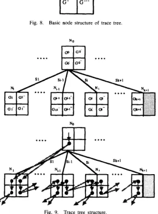
The reliability analysis process of the FREA algorithm can be represented by a trace tree. A trace tree depicts the relationship among intermediate trees or subgraphs generated using the reductions concepts incorporated in the FREA algorithm. A trace tree node consists of four components, G. G', G", and G"', as shown in Fig. 8, which represents the intermediate trees or subgraphs from the reduction process.
The relationship of trees within a trace tree node, using notation defined in FREA, can be explained by the following example. A trace tree is given in Fig. 9.
Suppose intermediate tree Gb in the trace node N o has started
node .rs with k incident edges, then the maximal number of trace tree nodes that trace tree node -1-0 can derive is k
+
1 (refer to (3)).92 IEEE TRANSACTIONS ON COMPUTERS, VOL. 43, NO. 1, JANUARY 1994
FREA ALGORITHM begin
G = the original DCS graph F N = U p , t p , \ FA\-, R = O
search a node x , that contains program P, E P S
if node s, is not found then
/* all the needed data files for program P, in P T */
/* the reliability set to 0 */
begin output(R) stop end s = 2 R = R E L ( G , ) output( R ) stop end (* FREA *) function REL(G,) begin
/* starting node’s number */
Step 1: The checking step
if F A ,
_>
F N and P A ,_>
PA\* thenbegin
R E L = 1 return
if there are no FST’s in G, then
end begin
/* using DFS algorithm to check this */
R E L = 0 return
/* no FST’s in G , */
end
Step 2: The reduction step for G,
repeat
Perform degree-I reduction Perform series reduction Perform parallel reduction
Perform degree-2 reduction /* using REDUCIBLENODE algorithm * I
Until no reductions can be made
Step 3: The formulating step for equation (3) 3.1:
3.2:
GL = the new graph after the above reduction
G’,” = GY = G’, R = O
C = l
for all s s , j E the set of edges incident on starting node .rs do
/* G’,I and GY are temporary variables for graph GI5 */ /* set reliability to 0 */
/* the constant terms,
. .
. q s . l q s . . . p , h . of equation (3) */c
= C ’ P S Jc
= c*q,,3.3: R = R
+
C* REL(G’,” .r, )G” - G$ - 3.4: s - x S J
3.5: G‘,“ = the new graph after deleting irrelevant components from GY if ss isdeleted then
go to step 4
Step 4: The choosing step to find the new staring node
od
if finding a node s k in G”’ that contains the programs under consideration then
begin s = k R = R -k C*REL(G$”) end REL = R end (* REL *)
IEEE TRANSACTIONS ON COMPUTERS, VOL. 43, NO. 1, JANUARY 1994 93
Since only k
+
1 terms (intermediate subgraphs) can be generated, components GY+l and G;kl within the trace tree node .\ik+l arenil. S, represents the operations to be applied from G’ in trace tree node YO to trace tree node N j . The operations available for S, can be deleting, merging, or combinations of merging and deleting. For example, S, = G x s , 2 means that edge ss 1 in component Gb is deleted and then Gb is merged with edge xs,2 to produce a new intermediate subgraph G, within trace tree node .Vj. The symbol + indicates which intermediate subgraph is generated by which intermediate subgraph. For example, G1 in trace tree node by applying operation SI (written as G1 = Gb@x, 1 using the notation defined in
FREA). The rest of the relations are listed at the bottom of the page. If the starting node I, in component G within trace tree node
LVj
holds all data files required and programs to be executed, then is a leaf node of the trace tree. Fig. 10 depicts the trace tree for program 1 to be executed in Fig. 1, where link 11 2 corresponds to link 1, links1,3 corresponds to link 2, . . . , etc.
is obtained from the Gb within trace tree node
DPRl can be computed as DPRi = p i
+
qipz(p3+
4 3 ~ s )+
~ 1 ~ 2 ~ 6 = p l+
q1p2 ( p 3+
93p5 = p l+
qlpZp3+
q l p 2 q 3 p S+
qlq2P3P4+
q l q 2 (p3p4+
pS - p3p1p5 )+
qlq2p.5 - qlqZp3p4pS.where p , is the probability of link I in Fig. 10, and qz = 1 - p , . computed to 0.99891.
Let the probability of any operational link be 0.9, then DPRl is
V. ALGORITHM COMPARISON
Unlike the li-terminal reliability problem, where li -terminal nodes are fixed and given, the distributed program reliability problem
does not have fixed I<-terminal nodes. The li -terminal nodes in the distributed program reliability analysis can dynamically be changed due to the effects of link or node failure, the ways of data files and program distribution, and the topology of the network. Therefore, we may say the network reliability problem is considered to be static-oriented while the distributed program reliability problem is dynamic-oriented. Naturally, the DPR problem is considered to be more complex and difficult than the computer network reliability problem. In fact, computing reliability of this type of problem has been known as a NP-hard problem.
In this section, comparisons with existing algorithms [6], [13], [14], [20] are given. The algorithms presented in [6], [13], [14], and [20], in the worst case, can generate as many as ( n
-
l)€-’ intermediate trees (or subgraphs), where n denotes the number of nodes and c is the maximum in-degree of a node in the graph. However, in practical conditions, it seldom occurs since once an MFST is found the tree expansion is stopped. The FREA algorithm employs the generalized factoring theorem with several reduction concepts to speed up the whole reliability evaluation. A rational comparison for these different algorithms can be made based on the counting approach, which counts the number of intermediate trees or subgraphs generated during the whole reliability evaluation. From such a comparison, one can approximate how much memory space and time units are required for their algorithms to run the distributed programs under the effects of different sizes of DCS, data file distributions, program distributions, and topologies. We also provide some actual execution results to support these analyses. The following subsections focus on these different comparisons.A. Effect of Different Sizes on Performance of Different Algorithms
Fig. 11 is a well-known example of a computer communication network-the ARPA computer network in which there are 21 nodes
REDUCIBLE-NODE (G) begin
for all node x, E G do begin
if degree ( 1 ~ ~ ) = 2 then
/* assume that the two edges incident on node .rl are .rl and s , k */ G I = G - x , ,
for all files f E ( F A , rlFA\-) and all program p E ( P A ,
n
P S ) do /* delete xt from G */delete all nodes in G1 that contain file f or program p from G 1 except node x t . G2 = the component that contains node x 2 in G1
if there are some FST’s in G2 then go to checkaextaode od
G l = G - x , k
the same as the above for-loop
I* delete I, k from G */ . .
. . .
. . ..
. . . .
. . . ..
/* the x 2 is a reducible node, apply degree-2 reduction */ G = G - X I - x , ] - I , k + , r : k
p:,k = p z 3 j
*
pz kFz4, = FA, U F A , (or F d k = FAk U F A , ) PA, = PA, U P A , (or Pd4k = PAk U P A , ) end
checkaextmode:
end (* REDUCIBLENODE *) od
94 IEEE TRANSACTIONS ON COMPUTERS, VOL. 43, NO. 1, JANUARY 1994 Leeend: series reduction $ degree-2 reduction
1
parallel reduction 0 starting nodeFig. 10. Trace tree of FREA for example of Fig. 1 .
and 26 links. Suppose that there are 12 data files and 10 programs distributed in the ARPA computer network, and the file distribution, program distribution, and files needed for a program to be executed are given in Tables I, 11, and 111, respectively. The number of subgraphs generated for different programs under consideration are given in Table IV.
It is clear that the FREA algorithm is thousands of times less than that of the existing algorithms in a large and complex distributed network such as ARPA.
B. Effect of Topology on Performance of Different Algorithms
In this study, we want to see the effect of topological configuration on the performance of different algorithms used. Thus, we run a different set of programs and file distributions over various topologies starting from a simple loop to a completely connected graph. These topologies are shown in Fig. 12, and the file distributions, program distributions, and data files needed for the program to be executed are given in Tables V, VI, and VII, respectively. These topologies, file
TABLE 1 FILE DISTRIBUTIONS Files Nodes F1 1 1 , 14, 19 F2 1 , 14, 21 F3 2, 5, 17 F4 9, 15 F5 6, 12, 20 F6 1, 5, 18 F7 3, 11, 15 F8 9, 16 F9 F10 F11 F12 10, 18 4, 10, 13 2, 7 8
distributions, and program distributions are the same as those used in [13]. Fig. 13 shows the number of subgraphs generated versus different topologies based on program 1 as executed at node 1.
G 1 = GO’ r S , 1
G1’ = the reduction graph of G 1 G I ” = G1’
-
S , 1G1”’ = the reduction graph of G1” Gi =
Gz”‘
- 1 1 .rs,
G I ‘ = the reduction graph of G / Gl’’ = Gl”’
-
1 - .r-. ,Gi”’ = the reduction graph of G!’ fori = 2.3.. . .
.
kGk
+
1 = Gk“‘ with a new starting nodeGk‘
+
1 = the reduction graph ofGli+
1I* step 3.2 and 3.3 * I I* step 3.1 * I I* step 3.5 * I /* step 3.3 *I I* step 3.1 * I I* step 3.4 * I I* step 3.5 *I I* step 3.1 * I /* step 3.2 and 3.4 * I /* step 4 *I
IEEE TRANSACTIONS ON COMPUTERS, VOL. 43, NO. 1, JANUARY 1994 95
SRI UTAH NCAR AWS CASE
Fig. 11. ARPA computer network. TABLE I1 PROGRAM DISTRIBUTIONS Programs Nodes P1 1 P2 14 P3 2 P4 15 P5 9 P6 21 P7 19 P8 6 P9 8 P10 4 TABLE 111
DATA FILES NEEDED FOR EXECUTING A PROGRAM
r,
~ _ _ _ _ _
Programs Files Required
P1 F1, F3, F5, F7 P2 F2, F4, F6, F8 P3 F9, F10, F11 P4 F10, F11, F12 P5 F6, F7 P6 F1, F6, F7 P7 F1, F8, F12 P8 F3, F4, F5, F6 P9 F1, F11 P10 F4, F8, F12
Other results also follow a similar curve and are reported in [21]. From these comparisons, it is clear that the FREA algorithm is the fastest (best) one, compared with the other algorithms, in any of these different topologies.
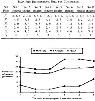
C. Effect of Data File Distributions on Performance
of Different Algorithms
Eight different sets of data file distributions, generated randomly based on the topology in Fig. 14 for the comparison of three algorithms, are listed in Table VIII. The program distribution and data files needed for the program to be executed are referred to Tables VI
and VII, respectively. Fig. 15 depicts that the number of subgraphs versus different data file distributions based on program 4 is executed at node 2. Other results also follow the similar curve and are reported in [21].
From the preceding comparisons, it is clear that the FREA algo- rithm has the best performance in these different data file distribu- tions.
D. Effect of Program Distributions on Performance of Different Algorithms
Fig. 16 shows the effect of programs running on different nodes based on the DCS in Fig. 14. The data file distributions and data files
12 x4 d 14
'2 14 12 14
16
r3 r5 13 IS
Fig. 12. Various topologies.
h g r a m 1 executed at node 1 .X.MFST[61 9 FARE[131 -FRFA 450 Number of 300 subgraphs 2.50 150 1 0 0 so generaled 200 Topology
Fig. 13. Number of subgraphs generated versus different topologies.
TABLE IV
NUMBER OF SUBGRAPHS GENERATED AND DPR
FOR EXAMPLE OF ARPA COMPUTER NETWORK
p2
P
i
Pl p5 Program Algorithm " MFST [6] 55700 70842 172907 197541 17292 FARE [13] 20007 13923 35515 38120 3300 FREA 412 57 70 184 75 DPR 0.9708450 0.9739356 0.9766832 0.9345704 0.9847566 p;r8
P9 PI 0 Program Algorithm " MFST [6] 39893 82759 44017 72005 257333 FARE [I31 13075 25135 11141 22436 66752 FREA 95 25 152 55 290 DPR 0.9334858 0.9143801 0.9821738 0.9703900 0.9695497needed for each program to be executed are referred to in Tables V
and VII, respectively. Other results also follow the similar curve and are reported in [21].
E. DPR Analysis of Running the Same Distributed Program from More than One Site
In this section, we compare the effect of the same program when executed from more than one site (node). From the example in Fig. 17, PI can be executed at node SI or .rc: P2 can be executed at node
96 IEEE TRANSACTIONS ON COMPUTERS, VOL. 43, NO. 1, JANUARY 1994 TABLE V FILE DISTRIBUTIONS Files Nodes F1 1, 2, 3 F2 2, 4 F3 3, 5 F4 3, 6 F5 1, 4 F6 5 TABLE VI PROGRAM DISTRIBUTIONS Nodes Program 1 P1 2 P4 3 P2, P3 4 P2, P3 5 P4 6 P1 x2 x4 X I x6 x3 xs
Fig. 14. Topology of DCS for 8-set of data file distributions.
120
T
A
*nh
generated 20 0 - T 1 2 3 4 5 6 7 8 File disaibutionsFig. 15. Number of subgraphs versus different data file distributions. TABLE VI1
DATA FILES NEEDED FOR EXECUTING A PROGRAM p, Programs Files Required
P1 F1, F2, F3
P2 F2, F4, F6
P3 F1, F3, F5
P4 F1, F2, F4, F6
.r~ or s p : P3 can be executed at node s3 or X I : PI can be executed at node .r2 or s5. Table IX shows the number of subgraphs generated
and the DPR of the same program to be executed from more than one node of the example in Fig. 17. FARE [13] is not applicable for distributed programs running at more than one node.
It should be noted that the current FARE algorithm [13] cannot compute DPR of the same program executed from more than one site.
TABLE VI11
DATA FILE DISTRIBUTIONS USED FOR COMPARISON
Set Set 1 Set 2 Set 3 Set 4 Set 5 Set 6 Set 7 Set 8 Files (nodes) (nodes) (nodes) (nodes) (nodes) (nodes) (nodes) (nodes)
Fi 2 , 4 , 5 2 , 3 , 6 4 , 5 , 6 1 , 2 , 3 1 , 4 , 6 1 , 3 , 6 3 , 4 , 5 2 , 3 , 6 F.r 4 , 5 3 , 5 2 , 3 4 , 5 2 , 5 3 , 6 1 , 2 3 , 5 Fs 5 , 6 3 , 4 4 , 5 1 , 6 3 , 4 1 , 2 5 . 6 1 , 6 F1 3 , 4 2 , 3 1 , 3 2 , 4 2 , 5 4 , s 5 , 6 2 , 6 F5 4 , 6 4 , 5 4 , 5 2 , 4 3 , 5 4 , 6 1.6 3 , 6 FG 6 3 6 3 5 5 5 4 Number of 20 svbnrmhs 1 2 3 4 5 6 me node w k r e pmg- I S ~ M J 11s exezution
Fig. 16. Number of subgraphs versus different program distributions TABLE IX
NUMBER OF SUBGRAPHS GENERATED A N D DPR FOR EXAMPLE OF FIG. 17
Pl pr
r?
PI Program Algorithm MFST [6] 42 98 58 103 FREA 30 22 27 58 - - - FARE [ 13) - DPR 0.9995076 0.9976697 0.9997831 0.9976616F. Actual Execution Time Comparison
Generally, an algorithm with less subgraphs generated during the DPR analysis will have better execution efficiency since the execution time required for the algorithm to analyze the reliability is dominated by the expanding steps (the recursive part) to generate subgraphs. When fewer subgraphs are generated during the analysis, it implies that the size of the original graph has been reduced before subgraph generation. Certainly, we expect that it will take less time to analyze a smaller graph. The time spent by reliability preserving reduction routines incorporated in the FREA algorithm is less significant than the subgraph expansion (the recursive part) which could grow exponentially. To support this observation, we provide some actual execution time comparisons among these algorithms. The compared algorithms are all implemented using the C program under the same hardware and software environments. The following execution results are the analysis of the distributed programs 1 to 10 in the ARPA network (Fig. 11) under the 1BM RISC/6000 workstation. It is clear that the proposed FREA algorithm outperforms existing algorithms in execution of any of these distributed programs.
VI. CONCLUSION
The distributed computing system (DCS) has become very popular for its high fault tolerance, potential for parallel processing, and better reliability performance. One of the important issues in the design of the DCS is the reliability performance. Traditional reliability
IEEE TRANSACTIONS ON COMPUTERS, VOL. 43, NO. I , JANUARY 1994 91
M 4 4 F I .FZ.F4,F6) Fig. 17. Example of the same program executed at more than one site.
TABLE X
EXFCUTION TIME (IN StCONDs) BY DIFFERENT ALGORITHMS FOR DISTRIBUTED PROGRAMS 1 TO 10 IN ARPA NETWORK UNDER IBM RlSCi6000 WORKSTATION
Algorithm Program I‘ r 2 p4 PI A MFST [6] 58.22 275.33 1462.69 >1800 15.59 FARE [ 13) 4.08 2.93 7.29 7.75 0.78 FREA 1.44 0.27 0.28 0.68 0.24 DPR 0.9708450 0.9739356 0.9766832 0.9345704 0.9847566 P, P,,
r,
0 Program Algorithm ‘I’ MFST [6] 03.31 474.28 104.00 246.17 >1800 FARE [13] 2.27 5.1 1 2.39 4.56 13.4 FREA 0.28 0.07 0.43 0.2 0.77 DPR 0.9334858 0.9 143801 0.9821738 0.9703900 0.9695497indexes such as source-to-terminal [ 7 ] , survivability [8], multiterminal reliability [ 101, and Zi-terminal reliability [ll] are not directly applicable for the analysis of the distributed reliability property in DCS without appropriate modification. Thus, new approaches and algorithms for the reliability analysis of the DCS must be developed. In this correspondence, we propose an algorithm, called the Fast Reliability Evaluation Algorithm (FREA), based on the generalized factoring theorem by employing several reliability preserving reduc- tions to speed up the reliability evaluation process. The use of the generalized factoring theorem implies that all subgraphs generated will be completely disjoint and, therefore, no replicated trees will be generated. The use of various reliability preserving reduction techniques implies that the size of the graph will be reduced and, therefore, less subgraphs will be generated. Compared with existing algorithms on various network topologies, file distributions, and program distributions, the FREA algorithm is much more economical in both time and space. This claim can also be supported by the actual execution time analysis reported in Section V-F. The feasibility of the proposed algorithm for distributed program reliability and distributed system reliability analyses can easily be confirmed by analysis on the ARPA computer network. The current FREA algorithm assumes that all nodes are perfect in its current analysis. For an imperfect node case, a slightly modified FREA algorithm can be used to generate all minimum file spanning trees, and then SYREL or a similar reliability package is called for the reliability evaluation. The more detailed treatment is reported in [21]. Also, the effect from task migration on the distributed program reliability is an important research issue, which we will study in the future.
REFERENCES
[ I ] D. P. Agrawal, Advanced Computer Architecture. Tutorial Text, IEEE Computer Society.
[2] T. C. K. Chou and J. A. Abraham, “Load redistribution under failure in distributed systems,” IEEE Trans. Comput., vol. C-32, pp. 799-808, Sept. 1983.
[3] D. W. Davies, E. Holler, E. D. Jensen, S. R. Kimbleton, B. W. Lampson, G. Lelann, K. J. Thurber, and R. W. Watson, “Distributed systems
architecture and implementation,” in Lecture Notes in Computer Science, vol. 105.
[4] P. Enslow, “What is a distributed data processing system?,” IEEE Computer, vol. 11, Jan. 1978.
(51 J. Garcia-Molina, “Reliability issues for fully replicated distributed database,” IEEE Computer, vol. 16, pp. 3 4 4 2 , Sept. 1982. [6] V. K. Prasnna Kumar, S. Hariri, and C. S . Raghavendra, “Distributed
program reliability analysis,” IEEE Trans. Sofhvare Eng., vol. SE-12, no. 1, pp. 42-50, Jan. 1986.
(71 A. Satyanarayna and J. N. Hagstrom, “New Algorithm for Reliability Analysis of Multiterminal Networks,” IEEE Trans. Reliability, vol. R-30, pp. 325-333, Oct. 1981.
[8] R. E. Merwin and M. Mirherkerk, “Derivation and use of survivability criterion for DDP systems,” in Proc. 1980 Nat. Comput. Conj, May 1980, pp. 139-146.
[9] K. K. Aggrawal and S. Rai, “Reliability evaluation in computer- communication networks,” IEEE Trans. Reliability, vol. R-30, pp. 32-35, Apr. 1981.
[IO] A. Grnarov and M. Gerla, “Multiterminal reliability analysis of dis- tributed processing system,” in Proc. 1981 Int. Conf Parallel Process- ing, Aug. 1986, pp. 79-86.
[ 111 R. Kevin Wood, “Factoring algorithms for computing I; -terminal network reliability,” IEEE Trans. Reliability, vol. R-35, pp. 269-278, Aug. 1986.
[I21 S. Hariri and C. S . Raghavendra, “SYREL: A symbolic reliability algorithm based on path and cutset methods,” USC Tech. Rep., 1984. [ 131 A. Kumar, S. Rai, and D. P. Agrawal, “Reliability evaluation algorithms
for distributed systems,” in Proc. IEEE INFOCOM 88, 1988, pp. 851-860.
[ 141 A. Kumar, S . Rai, and D. P. Agrawal, “On computer communication net- work reliability under program execution constraints,” IEEE J . Selected Areas Commun., vol. 6, no. 8, pp. 1393-1399, Oct. 1988.
[lS] F. Moskowitz, “The analysis of redundancy networks,” AIEE Trans. (Commun. Electron.), vol. 29, pp. 627-632, 1958.
[ 161 M. 0. Ball, “Computing network reliability,” Opf. Res., vol. 27, pp. 132-143.
[ 171 M. K. Chang, “A graph theoretic appraisal of the complexity of network reliability algorithms,” Ph.D. dissertation, Dept. of IEOR, Univ. of California, Berkeley, 1981.
[IX] A. Satyanarayana and M. K. Chang, “Network reliability and the factoring theorem,” Networks, vol. 13, pp. 107-120, 1983.
[ 191 R. K. Wood, “A factoring algorithm using polygon-to-chain reductions
for computing IC-terminal network reliability,” Networks, vol. 15, pp.
173-190, 1985.
(201 C. S. Raghavendra, V. K. Prasnna Kumar, and S. Hariri, “Reliability analysis in distributed system,” IEEE Trans. Comput., vol. 37, pp. 352-358, Mar. 1988.
[21] D. J. Chen, “On the reliability analysis of the distributed computing system,” Comput. Sci. Inform. Engineering, National Chiao Tung Univ., China, Tech. Rep. CSI-1991-005, July, 1991.