Land Vehicle Guidance
in Outdoor Road
Environments Using
Combined Line and Road
Following Techniques
● ● ● ● ● ● ● ● ● ● ● ● ● ● ● ● ● ● ● ● ● ● ● ● ● ● ● ● ● ● ● ● ● ● ●
Kuang-Hsiung Chen Wen-Hsiang Tsai*
Department of Computer and Information Science National Chiao Tung University
Hsinchu, Taiwan 300, R.O.C.
Received January 18, 1996; accepted May 13, 1997
An intelligent approach to autonomous land vehicle (ALV) guidance in outdoor road environments using combined line and road following and color information clustering techniques is proposed. Path lines and road boundaries are selected as reference models, called the model and the road-model, respectively. They are used to perform line-model matching (LMM) and road-line-model matching (RMM) to locate the ALV for line and road following, respectively. If there are path lines in the road, the LMM process is used to locate the ALV because it is faster than the RMM process. On the other hand, if no line can be found in the road, the RMM process is used. To detect path lines in a road image, the Hough transform is employed, which does not take much computing time because bright pixels in the road are very few. Various color information on roads is used for extracting path lines and road surfaces. And the ISODATA clustering algorithm based on an initial-center-choosing technique is employed to solve the prob-lem caused by great changes of intensity in navigations. The double model matching procedure combined with the color information clustering process enables the ALV to navigate smoothly in roads even if there are shadows, cars, people, or degraded regions on roadsides. Some intelligent methods to speed up the model matching processes and the Hough transform based on the feedback of the previous image information are also presented. Successful navigations show that the proposed approach is effective for ALV guidance in common roads. 1997 John Wiley & Sons, Inc.
*To whom all correspondence should be sent.
Journal of Robotic Systems 14(10), 711–728 (1997)
1. INTRODUCTION
unsupervised clustering technique.20A shrink andex-pand algorithm21was used to remove small regions.
Autonomous land vehicles (ALVs) are useful for A minimum distance criterion based on a Grassfire many automation applications. Successful ALV navi- transformation22is used to obtain the most reasonable
gation requires integration of techniques of environ- interpretation. EDDIE7 was a software architecture
ment sensing, ALV location, path planning, wheel that combined separate functional parts like sensing, control, etc. This study is mainly concerned with ALV planning, and control into an intelligible system. Ad-guidance in outdoor road environments using com- ditionally, Kluge and Thorpe3split the assumptions
puter vision techniques. Many techniques have been made in road modeling into three loose classes: sub-proposed for ALV guidance in outdoor roads1–15and conscious, implicit, and explicit models. Moreover, a
indoor environments.16–19 In outdoor environments, new road tracking system called FERMI was designed
to explain explicit models and their purposes. because of the great variety of road conditions like
VITS9 and Navlab2 both used color information
shadows, degraded regions, moving objects, changes
in RGB planes for road following. Turk et al.9showed
of illumination, and even rain, we need to combine
that the G-component is redundant in their road anal-different problem-solving algorithms and perhaps
ysis. Navlab2deduced both color and texture
segmen-equip multiple sensors to solve the complex problem
tation results using a pattern classification method of ALV guidance in roads.
involving the mean and the covariance matrix. Lin The CMU Navlab1–8 is a system with several
and Chen10divided roads into three clusters: sunny
function-oriented categories such as SCARF, YARF,
road, shadow road, and nonroad. Their classification ALVINN, UNSCARF, and EDDIE. SCARF6,8handled
is based on the Karhunen-Loe`ve transform in the HSI unstructured roads. It recognized roads having
de-color space. The Germanic vision system11–13 used a
graded surfaces and edges with no lane markings
high-speed vision algorithm to detect road border in shadow conditions. It also recognized intersec- lines. The system has carried out both road following tions automatically with no supervised information. and vehicle following in real time. Kuan, Phipps, and YARF6dealt with structured roads. It guided
individ-Hsueh14 proposed a technique with transformation
ual trackers using an explicit model of features. It and classifier parameters being updated continuously could drive the vehicle on urban roads at speeds up and cyclically with respect to the slow change of color to 96 kph, which is much higher than the speed of and intensity. Hughes Research Laboratories15
de-SCARF. ALVINN4,6 preprocessed input images, put
signed a planning method using digital maps to route them to a neural net, and instantly obtained the wheel a desired path. When the vehicle went through the angles from the network. UNSCARF5separated un- path, sensors were used to provide environmental
de-scriptions. structured roads into homogeneous regions using an
In this article, we propose an intelligent approach to ALV guidance in outdoor road environments using combined line and road following and color informa-tion clustering techniques. Although a road scene is often uncertain and noisy in an outdoor environment, there are still stable features that can be extracted from a road image for use as reference models. Hence, model matching is a quite reasonable approach for ALV guidance in outdoor environments. We use path lines and road boundaries, which are apparent in common roads, to construct reference models, called the line-model and the road-model. Line-model matching (LMM) and road-model matching (RMM) are then used to locate the ALV for line and road following, respectively. Because the LMM process is much faster than the RMM process, the system
al-ways uses the LMM process to locate the ALV if any Figure 1. The prototype ALV used in this study. path line is detected. Only when no path line exists
does the system use the RMM to guide the ALV. By combining the two matching processes in this way,
A new prototype ALV (whose dimensions are faster and more flexible navigations in general roads
118.5 by 58.5 cm) with smart, compact, and ridable can be achieved.
characteristics, as shown in Figure 1, is constructed Furthermore, various color information on roads
as a testbed for this study. It has four wheels in which is used in this study to extract path lines and road
the front two are the turning wheels and the rear two surfaces. For this, the ISODATA algorithm20based on
the driving wheels. Above the front wheels is a cross-an initial-center-choosing (ICC) technique is
em-shaped rack on which some CCD cameras are ployed, which can solve the problem caused by great
mounted, and above the rack is a platform on which changes of intensity in navigations. Proper initial
cen-two monitors, one being the computer monitor and ters are chosen as the clustering algorithm begins to
the other the image display, are placed. Above the run. To detect path lines in a road image, the Hough
platform is a vertical bar on which another camera transform23is used, which can find the path lines in
used for line and road following in this study is the image even though they are dotted or noisy. The
mounted. The central processor is an IBM PC/AT transform does not take much computing time
be-cause bright pixels in the road are very few. compatible personal computer (PC486) with a color image frame grabber that takes 512 3 486 RGB im-The above double model matching procedure
combined with the color information clustering pro- ages, with eight bits of intensity per image pixel. The ALV is computer-controlled with a modular cess enables the ALV to navigate on the road
smoothly even though there are shadows, cars, peo- architecture, as shown in Figure 2, including four components, namely, a vision system, a central proc-ple, or degraded regions on the roadsides. Besides,
some intelligent methods to speed up the model essor PC486, a motor control system, and a DC power system. The vision system consists of a camera, a TV matching processes and the Hough transform, based
on the feedback of the previous image information, monitor, and a Targa Plus color image frame grabber. The central processor PC486 has an RAM with two are also presented. The proposed approach is proved
effective after many practical navigation tests. mega bytes, one floppy disk, a 120-mega-byte hard disk, a 300-mega-byte hard disk, and an EL slim dis-The main difference of our approach from
ex-isting methodologies is that the proposed system can play. The motor control system includes a main con-trol board with an Intel 8085 concon-troller, a motor switch visual features dynamically at the appropriate
time during navigation for improving the system’s driver, and two motors. The power of the system is supplied by a battery set including two 12-volt power efficiency. And different visual features can be
ex-tracted directly from the clustering result. Also, new sources, each being divided into various voltages us-ing a DC-to-DC converter set to provide power to and effective model matching methods are used to
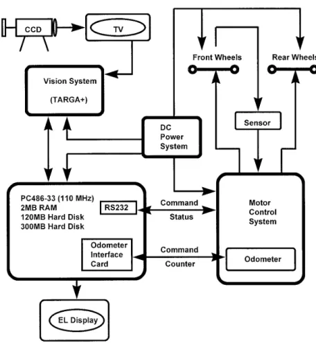
Figure 2. System structure of prototype ALV.
The remainder of this article is organized as fol- termine the ALV location. If any path line is detected in the road, the LMM process is used to guide the lows. In section 2, the details of the proposed
model-based ALV navigation method is described. In section ALV because it is faster than the RMM process. On the other hand, if no line can be found in the road, 3, the details of the proposed ALV location method
is introduced. The description of the used image pro- the RMM is used.
In the following, we first describe the steps of cessing techniques is included in section 4. In section
5, the results of some experiments are described. Fi- model creation, which involve several coordinate sys-tems and coordinate transformations. Then, the line-nally, some conclusions are made in section 6.
model matching process for line following and the road-model matching process for road following are introduced, followed by a description of the
com-2. PROPOSED MODEL-BASED ALV
bined line and road following technique.
NAVIGATION METHOD
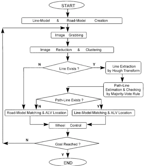
The proposed navigation scheme is performed in a 2.1. Model Creation cycle by cycle manner. An overview of the proposed
approach is shown in Figure 3. To finish each naviga- Several coordinate systems and coordinate transfor-mations are used in this approach. The coordinate tion cycle, the system identifies some stable features
in the road environment to locate the ALV, and plan systems are shown in Figure 4. The image coordinate system (ICS), denoted as u-w, is attached to the image a smooth path from the current position of the ALV
to the goal (or to a given navigation path). After the plane. The camera coordinate system (CCS), denoted as u-v-w, is attached to the camera lens center. The two reference models are created, the system
attached to the middle point of the line segment with the interval of 28. So, the line-model contains 233 17 5 391 line-templates, and each line-template which connects the two contact points of the two
front wheels with the ground. The x-axis and y-axis represents one specific ALV location.
We use the same method to create the road-are on the ground and parallel to the short side and
the long side of the vehicle body, respectively. The model. The road-model also contains 233 17 5 391 road-templates, and each road-template ROADij[al,
z-axis is vertical to the ground. The transformation
between the CCS and the VCS can be written in terms bl, ar, br] also represents an ALV location (di,uj). The
transformation is shown in Fig. 5(b). Thus, each ALV of homogeneous coordinates18–19, 26as
location T 5 (di, uj) can be represented by a
line-(u v w 1)5 template LINEij[al, bl, am, bm, ar, br] or a road-template ROADij[al, bl, ar, br], and vice versa. We say that
line-template (or road-line-template) Ti5 (di,ui) is similar to
line-template (or road-template) Tj5 (dj,uj) (denoted
(x y z 1)
3
1 0 0 0 0 1 0 0 0 0 1 0 2xd 2yd 2zd 143
r11 r12 r13 0 r21 r22 r23 0 r31 r32 r33 0 0 0 0 14
, (1) by Ti> Tj) if and only if udi2 dju # 25 (cm) and uui2uju # 2 (degree). (3)where Because the line-templates and the road-templates are
represented in the ICS, the model matching processes r115 cosucosw1 sinusinfsinw, described in the following are also operated in the
ICS. r125 2sinucosf,
r135 sinusinfcosw2 cosusinw, 2.2. Line-Model Matching for Line Following
r215 sinucosw2 cosusinfsinw, When path lines exist in the road image, they are
extracted and matched with a few candidate line-r225 cosucosf,
templates in the line-model, i.e., the LMM is per-r235 2cosusinfcosw2 sinusinw, formed. Without loss of generality, we first take the
extracted left path line to perform the matching if the r315 cosfsinw,
path line exists. We want to find the line-template TL
whose left path line is the most similar to the extracted r325 sinf,
left path line. We define the following similarity r335 cosfcosw, (2) measure
where uis the pan angle,fthe tilt angle, and wthe S5 1/[a ? uat2 aeu 1 b ? ubt2 beu] (4) swing angle, of the camera with respect to the VCS;
wherea and b are two weighting coefficiencies, and and (xd, yd, zd) is the translation vector from the origin
aeand atare the slopes, and beand btare the intercepts,
of the CCS to the origin of the VCS.
of the extracted left path line and the left path line An ALV location can be represented by two
pa-of the candidate line-template, respectively. Then, the rameters (d,u), where d is the distance of the ALV to
desired line-template TL5 (dL,uL) is the one that has
the central path line in the road anduis the pan angle
the maximum S value. If the extracted path lines of the ALV relative to the road direction (positive to
include the middle or the right path line, we use the the left). The equations of the three path lines on the
same criterion to obtain their corresponding most-road in the VCS are assumed to be known. Then, we
similar line-templates TM 5 (dM, uM) and TR 5 (dR,
transform them into the ICS, which is displayed on
uR), respectively. After TL, TMand TR are computed,
the TV monitor. For each ALV location (di, uj), we
the most meaningful ALV location T is derived by can create the corresponding line-templates LINEij[al,
the following majority-vote rule. bl, am, bm, ar, br], where al, am, and ar are the slopes,
and bl, bm, and br are the intercepts of the equations Case I(TL, TM, and TRare all similar): of the left, middle, and right path lines in the ICS,
respectively. The transformation is shown in Figure if TL> TM> TR,
5(a). We sample the road width at 23 positions with
then set T5 (TL1 TM1 TR)/3
the interval of 25 cm. At each position, we sample
Figure 3. An overview of the proposed approach.
Case II(only two of TL, TM, and TR are similar): the ALV. Similarly, we can locate the ALV using the
right and the middle lines if noise appears on the left if only Ti> Tj(i? j, i, j 5 L, M, R), roadside. Moreover, if noise exists on both sides, the
middle line, which is seldom affected by shadows or then set T5 (Ti1 Tj)/25 ((di1 dj)/2, (ui1uj)/2);
other noise, can also be used to locate the ALV. Fi-nally, when no line can be found on the road, we can Case III(TL, TM, and TRare not similar to each other):
perform the road-model matching process (described if TKis the most similar to the reference line-tem- later) to locate the ALV. Hence, we can locate the
plate (i.e., with the maximum S value) where K5 ALV even when there are shadows, people, cars, or L, M, or R, then set T5 TK. degraded regions on the roadsides. This flexible
guid-ance process makes the ALV navigation steady. The The reference line-template mentioned above is LMM algorithm is described below.
the one at the reference ALV location estimated by the system at the beginning of each navigation cycle.
The estimation of the reference ALV location will be LMM Algorithm described later. If no noise exists on the road, we can
derive a very accurate ALV location because three Input: A set E of extracted path lines and a set U of candidate line-templates.
lines can be used. If noise appears on the right
derive the most meaningful ALV location T ac-cording to the majority-vote rule described above.
It is not necessary to use the entire line-model to perform the matching with the extracted path lines. We only use the neighboring ones in the model around the reference line-template to save computing time. To analyze the time requirement of the LMM algorithm, let
1. the number of the candidate line-templates to perform the matching be k1;
2. the time to compute the similarity value be k2; 3. the time to run the algorithm of the
majority-vote rule be k3,
Figure 4. The three coordinate systems ICS, CCS, and VCS.
where k1is constant, and k2and k3can be easily shown
Step 1. For each extracted path line y5 aEx1 bEin E: to be constants by observing Eq. (2) and the
majority-(a) for each candidate line-template LINEij[aL, bL, vote rule, respectively. The time to process Step 1(b)
aM, bM, aR, bR] in U: in the LMM algorithm using the sequential search
compute Sij5 1/[a ? uaE2 aKu 1 b ? ubE2 bKu], algorithm can easily be shown to be k1.27 Then, for
where K5 L, M, or R; each extracted path line, the time to calculate the (b) for all of the computed Sijvalues: similarities of all the candidate line-templates plus
use the sequential search algorithm to find the time to find the best line-template having the the best-matched line-template TKhaving the maximum S
ijvalue can be calculated by
largest Sijvalue, where K5 L, M, or R.
Step 2. From all of the obtained best-matched
line-templates (with the number at most three): TL15 k13 k21 k1. (5)
Figure 5. The transformation between the VCS and the ICS. (a) Path line transformation. (b) Road boundary transformation.
Because there are at most three path lines that can be extracted and Step 2 takes k3time, the total time
used by the LMM algorithm can be calculated by TL5 3 3 TL11 k3
5 3 3 k13 k21 3 3 k11 k3 (6)
which is a constant. Consequently, the time complex- Figure 6. The matched road-template represented by the ity of the LMM algorithm is of the order O(1), which two black lines based on the MBPNM criterion.
does not depend on the image size.
2.3. Road-Model Matching for Road Following
If the best-matched road-template is not similar If no high peak is found in ther2uHough counting
to the reference road-template at the reference ALV space, or if the extracted line-templates are not similar
location, we assume that the visual features are miss-to each other and none of them is similar miss-to the
refer-ing in the present navigation cycle and drive the ALV ence line-template, we conclude that no path line
blindly, i.e., using only the vehicle control informa-exists on the road. We then perform the more
time-tion. If such a case happens for several continuous consuming road-model matching (RMM) based on a
navigation cycles, we assume that the vision system criterion proposed in this study, called the
maximum-has lost its function and the vehicle is stopped. As bounded-pixel-number matching (MBPNM)
de-an example, a binary image showing the cluster-1 scribed as follows. Basically, a road can be divided
pixels and the best-matched road-template repre-into three clusters: (1) cluster-0: dark area, like
shad-ows and trees; (2) cluster-1: gray area, coming from sented by the two black lines obtained with the the main body of road; (3) cluster-2: bright area, like MBPNM criterion is shown in Figure 6. It can be seen the sky and the white or yellow lines on the road. that the shadow area is included in the bounded-We define the bounded-area for each navigation cycle area, i.e., it is regarded as part of the road. So, we as that bounded by the two lines of the road-template, can say that the adopted MBPNM criterion is not and the bounded-pixels as those belonging to cluster- sensitive to shadows. Also, we do not use the entire 1 (most likely to be the road area) in the bounded- road-model to do the matching because it wastes too area. If a road-template includes within its bounded- much time. We only use the neighboring ones in the area the largest number of bounded-pixels, it can be model around the reference road-template (forming regarded as the one most likely to be the road bound- the set W in the above RMM algorithm) to perform ary shape, i.e., as the best-matched road-template. the matching. To analyze the time requirement of the The RMM algorithm based on MBPNM is de- RMM algorithm, let
scribed below.
1. the image size be I5 m 3 n pixels;
2. the number of the candidate road-templates RMM Algorithm
be k1;
Input: A set V of pixels belonging to cluster-1 and a 3. the number of the pixels in the bounded-area set W of candidate road-templates. of the road-template T
i be Bi 5 ci 3 I with
Output: The most meaningful ALV location T. c
i, 1;
Step 1. For each candidate road-template Ti in W: 4. the number of the bounded-pixels of the
road-(a) initialize the number of bounded-pixels template T
ibe Ni5 di3 Biwith di, 1;
Ni5 0; 5. the time to check whether one pixel belongs
(b) for each pixel pj in the bounded-area of Ti: to cluster-1 or not be k 2; and
if pj is also in V, then set Ni5 Ni1 1.
6. the time to increment a variable be k3,
Step 2. For all of the computed Ni values:
use the sequential search algorithm to find the
best-matched road-template T having the largest where k1, k2, k3, ci, and diare constants. Then, the time
to calculate all the numbers of bounded-pixels of all Nivalue and take T as the desired output.
the candidate road-templates (Step 1 in the RMM Output: The ALV location T. algorithm) can be expressed as
Step 1. Initialization:
(a) Initialize Error-flag5 0.
(b) Check in I the surrounding area A of the TR15
O
k1
i51
O
Bi
j51[k21 (Ni/Bi)3 k3] three lines of the reference line-template. (c) If pixels belonging to cluster-2 in the
sur-rounding area A are insufficient (i.e., if area 5
O
k1
i51
O
ci3m3n
j51 [k21 di3 k3] A> V2is too small), then go to Step 3.
Step 2. LMM:
(a) Extract a set L of path lines from V2 by the
5
O
k1
i51((k21 di3 k3)3 ci3 m 3 n) (7) Hough transform.
(b) Use L and U as the inputs to run the LMM which is of the order O(mn). Also, the time to perform algorithm to find the candidate ALV
loca-Step 2 can be expressed as tion Tc.
(c) If Tcis similar to the reference line-template,
TR25 k1 (8) then go to Step 4.
Step 3. RMM:
(a) Use V1and W as the inputs to run the RMM
which is of the order O(1). Hence, the total time of
algorithm to find the candidate ALV loca-the RMM algorithm can be calculated by
tion Tc.
(b) If Tcis not similar to the reference
road-tem-TR5 TR11 TR2 (9)
plate, then set Error-flag5 1. Step 4. End of cycle:
which is of the order O(mn)1 O(1) or simply O(mn).
If Error-flag5 0, then set T 5 Tc; otherwise set
Consequently, the time complexity of the RMM
algo-T5 reference ALV location and print ‘‘all visual rithm depends on the image size.
features are missing.’’
The purpose of including Steps 1(b) and 1(c) is 2.4. Combination of Line and Road Following
to save computing time. If pixels belonging to cluster-If only path lines or only road surfaces are selected as 2 in the surrounding area are insufficient, we con-visual features, navigation may still be accomplished. clude that no path line exists on the road and ignore But because we have shown that the LMM algorithm line extraction, and perform the RMM algorithm im-is much faster than the RMM algorithm, we prefer mediately. On the other hand, if there are enough line following to road following if there are path lines pixels in the area, line extraction and the LMM algo-on the road, to accomplish faster navigatialgo-on. On the rithm are performed to derive a candidate ALV loca-other hand, if only path lines are used, the vehicle tion Tc. If Tcis not similar to the reference line-tem-cannot navigate on roads without path lines. Hence, plate, the LMM algorithm becomes unreliable and the we employ a combined technique to achieve faster RMM algorithm is then used. Finally, if the candidate and more flexible navigations. The details are de- ALV location resulting from the RMM algorithm is scribed by the following combined line and road not similar to the reference road-template, the RMM model matching (CLRMM) algorithm. algorithm becomes unreliable, too. At this moment, all of the desired visual features are missed and the ALV is guided blindly.
CLRMM Algorithm Input:
(a) A road image I.
3. PROPOSED ALV LOCATION METHOD
(b) The reference line-template and the reference
road-template. 3.1. Reference ALV Location Estimation (c) Two sets V1 and V2 of pixels belonging to
cluster-1 (road area) and cluster-2 (path lines) The ALV keeps moving forward after an image is taken at the beginning of each navigation cycle. When in I, and two sets W and U of candidate
road-templates and candidate line-road-templates, re- the image has been processed and the LMM or RMM algorithm has been performed, the actual ALV loca-spectively.
tion at the time instant of image taking can be found. At this moment, however, the ALV has already trav-elled a distance S. Hence, the ALV never knows its actual current position unless the cycle time is zero. To overcome this difficulty, we use the following information to estimate the current ALV location ac-cording to a method proposed by Cheng and Tsai:16 1. The obtained actual location (di,uj) at the time
instant of image taking. 2. The travelled distance S.
3. The pan angle d of the front wheels relative to the y-axis of the VCS.
4. The distance d between the front wheels and the rear wheels.
Figure 7(a) illustrates the navigation process, where Bi and Ei are the beginning and the ending
times of cycle i , respectively. At time Bi, an image is
taken and the current ALV location is assumed to be Pi. At time Ei, Piis found but the current ALV location
Pi11is unknown. At this moment, we use the control
information given above to estimate the current ALV location called Pi11. As shown in Figure 7(b), the
vehi-cle is located at Pi. What we desire to know is the
relative location of Pi11 with respect to Pi, denoted
by a vector T. By the basic kinematics of the ALV, the rotation radius R can be found to be
R5 d/sind. (10) And anglec can be determined by
c 5 S/R, (11)
where S can be obtained from the counter of the system odometer. So, the length of vector T can be solved to be
lT5 RÏ2(1 2 cos c), (12)
Figure 7. Illustration of reference ALV location estimation. and the direction of T is determined by the angle (a) The navigation process in a cycle by cycle manner. (b) The vehicle location before and after the ALV moves a distance S forward.
eT5 f
22d2 c2. (13)
So, in cycle i, Pi and P9i11 can be determined at time
Using the vector T, the VCS coordinates of location
Ei. And the estimated ALV locations at time Bi11can
P9i11with respect to Pican thus be computed by be set to P9
i11. We then define
x5 lTcoseT, Reference ALV location of cycle i
5 the estimated ALV location at time Bi. (15)
Hence, P9i11is used as the reference ALV location of Next, it should be mentioned that allowing the
ALV a larger angle to turn in a session of turn drive cycle i11. The reference ALV location can be used
for the following purposes: does not mean that better navigation can be achieved. It may cause serious twist. On the other hand, a smaller range of turn angles may cause only a slight 1. Speeding up the algorithms of line checking closeness to the given path. Hence, the largest angle and extraction. allowing the ALV to turn is a tradeoff between 2. Speeding up the LMM and the RMM algo- smoothness of navigation and closeness to the given
rithms. path. In our experiment, we found through many
3. Driving the ALV to the given path. iterative navigations that a turn from 258 to 158 is a good compromise.
Finally, we discuss the problem of ALV speed adjustment on varying road situations. When the 3.2. Path Planning
ALV meets ascending or descending roads, its speed To guide the ALV to following a given path, we have will become slower or faster, respectively. To keep to plan a smooth trajectory for the ALV from the the speed steady, we propose a solution as follows. current estimated ALV location to the given path in As we guide the ALV in navigation cycle i, we can each navigation cycle. For this, a closeness distance find its travelled distance Si, the elapsed time Ti, and
measure from the ALV to the given path proposed its driving power Piby checking the system encoder,
by Cheng and Tsai16is employed, which is defined as
the system clock, and the motor controller provided by the control system, respectively. Then, the speed of the ALV in cycle i can be calculated by
Lp(d)5 1 11 [DF P(d)]21 [DBP(d)]2 (16) Vi5 Si/Ti. (17)
Assume that we want to drive the ALV at a constant where DF
Pand DBP are the corresponding distances
speed V. Then, if Vi. V, it is decided that the ALV
from the front and the rear wheels of the ALV to the
is on a descending road. One way to derive a new given path after the ALV traverses a distance S with
driving power Pi11for the ALV is:
the turn angledas shown in Figure 8. A larger value of Lp means that the ALV is closer to the path. It is
easy to verify that 0, LP# 1, and that LP5 1 if and
Pi115
S
VVi
D
Pi. (18)
only if both of the front wheels and the rear wheels of the ALV are located just right on the path.
To find the turn angle of the front wheel to drive the ALV as close to the path as possible, a range of possible turn angles are searched. An angle is hypoth-esized each time, and the value of LP is calculated
accordingly. The angle that produces the maximal value of LPis then used as the turn angle for safe
navi-gation.
3.3. ALV Control Issues
There is always unavoidable mechanical inaccuracy within the ALV control system. If we only use the control information to drive the ALV, the ALV may be far away from the goal when the navigation ends. Hence, we employ computer vision techniques to ex-tract stable visual features as auxiliary tools to avoid
gradual accumulation of control error. Of course, con- Figure 8. Illustration of closeness distance measure trol error still exists in each navigation cycle. LP(d) 5 1/h1 1 [DFP(d)]21 [DBP(d)]2j.
Similarly, if Vi, V, the ALV is on an ascending road. of the same size as shown in Figure 9, i.e., for all
k5 0, 1, and 2, we have And Pi11can be calculated by
Pi115
S
VViD
Pi. (19)O
r9k s5rk [pixel no. of g.l.(s)]5O
rk11 t5r9k [pixel no. of g.l.(t)]. (20) We then use Pi11as the new driving power for cyclei1 1. where g.l. means gray level. Then, r9
k is taken to be
the R-component of the candidate center of cluster k. Using the same criterion on the G-plane and B-plane, we can find the G-component g9k and B-component
4. IMAGE PROCESSING TECHNIQUES
b9k. We then use [r9k, g9k, b9k] as the initial center of
The general purpose of image processing is to extract cluster k to run the unsupervised clustering algo-useful features from input images. Some forms like rithm, where k 5 0, 1, 2.
region-based or edge-based descriptions can be se- When navigation begins, it is not a good policy lected for use as representations of such features. We to run the unsupervised clustering algorithm again use a clustering algorithm and a line extraction because it needs about 10 to 20 iterations, which take method as the main image processing techniques to too much computing time, to finish its convergence find such descriptions in our study. Moreover, color and is unsuitable for real-time ALV navigation. is a powerful descriptor that often simplifies object Hence, we simply run the clustering algorithm for extraction and identification from a scene, so we use only three iterations, which is enough to gain ideal color features in the clustering algorithm. To solve clusters if we can choose proper initial centers. Intu-the problem caused by great changes of intensity, we itively, we can select the resulting centers in the pre-also propose a technique to acquire better clustering vious navigation cycle as the initial centers in the results by choosing suitable initial cluster centers for current navigation cycle to run the supervised clus-the clustering algorithm. The proposed color informa- tering algorithm.
tion clustering algorithm and the line extraction tech- The selection may be unsuitable, producing unac-nique are described as follows. ceptable clusters, because some difference may exist between two continuous images. One kind of the difference comes from the change of intensity. If the 4.1. Color Information Clustering
change of intensity between two continuous images is great (resulting from clouds covering the sun unex-The original image size is 512 3 486. To speed up
our algorithms, we have to reduce the image size. pectedly, for example), the candidate initial centers chosen from the resulting centers in the previous The upper portion in the road image is discarded
because it does not contain any road area, and pixels cycle may be far away from their real centers. In this situation, three iterations are not enough for the are sampled from the remaining image with the
inter-val of five pixels in both the horizontal and vertical ISODATA algorithm to move the candidate initial centers close to their real centers, and erroneous clus-directions to form a reduced 103 3 45 image. We
then use the ISODATA algorithm,20based on an ini- ters may be produced.
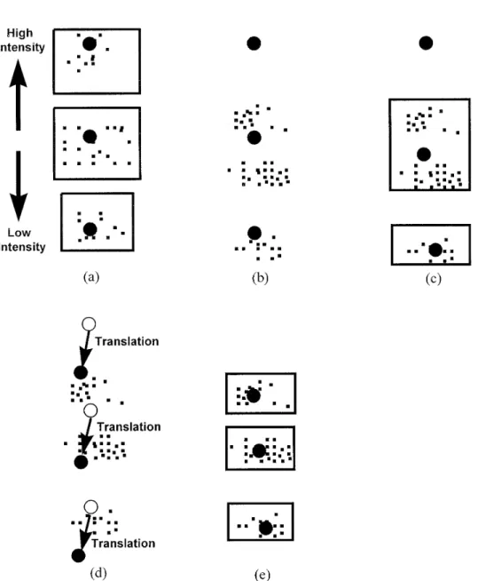
Furthermore, the number of clusters may de-tial-center-choosing (ICC) technique that can solve
the problem caused by great changes of intensity in crease and an even more serious problem happens. Figure 10 illustrates this situation. Figure 10(a) shows navigations, to divide the road image into three
clus-ters. Because the clustering result is sensitive to the the distribution of the three clusters and their re-sulting centers (represented by the big black dots) in choice of initial centers, it is necessary to choose
suit-able initial centers as the algorithm begins to run. the previous cycle. Figure 10(b) shows the greatly-translated distribution of the pixels caused by great The ICC technique is described below.
Before ALV navigation, we run an unsupervised changes of intensity in the present cycle, where black big dots represent the candidate initial centers inher-clustering algorithm that is guaranteed to converge
after several iterations by choosing proper initial cen- ited from the resulting centers in the previous cycle. After we run the supervised clustering algorithm for ters. The choice of appropriate initial centers is
de-scribed as follows. We first observe the histogram of three iterations in the present cycle, we obtain the clustering result shown in Figure 10(c), which is erro-the R-plane, and divide all erro-the pixels into six pieces
Figure 9. The histogram of the R-plane where r9k is the R-component of the center of
cluster k.
neous because one cluster becomes null and only two 11. Figure 11(a) shows the input image with high intensity in the previous cycle and Figure 11(b) shows clusters contain samples.
To solve this problem, we perform a translation the input image with low intensity in the present cycle. Figure 11(c) shows the poor clustering result on the resulting centers in the previous cycle to form
more representative points that are then selected for when the above translation process is not employed. One cluster becomes null in the result. A nice cluster-use as the actual candidate initial centers in the
pres-ent cycle. The translation is described as follows. As- ing result obtained from the translation process is shown in Figure 11(d), in which we see that cluster-sume that R9ave, G9ave, and B9aveare the averages of the
R-components, the G-components, and the B-compo- 1 is the road area and cluster-2 the path lines. This observation again justifies our use of a combined line nents of all the pixels in the previous input image,
respectively, and Rave, Gave, and Baveare the averages and road following technique.
of the R-components, the G-components, and the B-components of all the pixels in the present input
image, respectively. A translation vector is defined by 4.2. Path Line Extraction Using Hough Transform Generally, two effective methods can be used for line [Dr, Dg, Db]5 [Rave2 R9ave, Gave2 G9ave, Bave2 B9ave]. (21) extraction. One is the Least-Square (LS) line
approxi-mation24,25and the other is the Hough transform.23The
If the resulting center of cluster k in the previous cycle Hough transform can extract lines in any direction is [R9ki, G9ki, B9ki] , k5 0, 1, 2, then, the translated candi- automatically even though they are dotted, whereas
date initial center of cluster k is taken to be the LS line approximation has to select proper pixels before approximating lines and hence complicate [Rki, Gki, Bki]5 [R9ki, G9ki, B9ki]1 [Dr, Dg, Db]. (22) coding and debugging. But if many candidate pixels
in the XY plane are sent to the Hough counting space, it will take too much computing time. Hence, time is Figure 10(d) shows the translation process, where the
the vulnerability of the Hough transform. From an black big dots represent the new translated initial
observation of Figure 11, we find in the binary image centers. We then use the new translated centers as
that cluster-2 pixels are few and discontinuity exists the new candidate initial centers to run the supervised
between pixels, so the Hough transform is a proper clustering algorithm, and a much better clustering
line extraction method. result is shown in Figure 10(e).
Before line extraction, the surrounding area of An example of obvious improvement obtained
the three lines of the reference line-template is from using the above initial cluster center translation
Figure 10. The influence of great changes of intensity and its solution. (a) The distribution of the three clusters and their converged centers in the previous cycle. (b) A greatly-translated distribution of the pixels caused by great change of intensity in the present cycle, where black big dots represent the candidate initial centers inherited from the resulting centers in the previous cycle. (c) The distribution of the three clusters after running the supervised clustering algorithm for three iterations in the present cycle, with one cluster becoming null, causing a serious problem. (d) The translation process, where new translated initial centers are selected according to Eqs. (21) and (22). (e) A much better clustering result with three ideal clusters is obtained after using the new translated initial centers to run the clustering algorithm.
to cluster-2 in the surrounding area are insufficient, there are three path lines on the road. But because of some unsteady road conditions such as shadows, we conclude that no path line exists on the road and
line extraction is ignored. If there are enough pixels degraded regions, or cars on the roadsides, we may only find one or two high peaks corresponding to in the area, we decide that there are path lines on the
road and send the candidate pixels to the Hough one or two lines with which we still can locate the ALV by using the majority-vote rule described pre-counting space to extract path lines. Normally, three
5. EXPERIMENTAL RESULTS
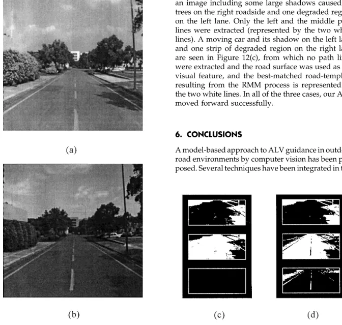
time is about 2.1 s, and the average speed is 90 cm/s or 3.3 km/h, which is reasonable for the small-scaled The prototype ALV constructed in this study was and PC-based ALV. The ALV can navigate steadily used for testing the proposed approach, and could in spite of the fact that there were shades, vehicles, navigate smoothly along part of the campus road in people, or degraded regions on the roadsides. National Chiao Tung University for about 150 m. Figure 12 shows some images and their clustering Besides, it is not sensitive to sudden changes of inten- results in several complex road environments. Figure sity because of the effective ICC technique used in 12(a) shows a road image that includes some small the clustering algorithm. The width of the road is shadows caused by trees on the left roadside and 6.8 m, and there are three yellow path lines on the some degraded regions on the left lane. All of the road with the central line dotted. The average cycle three path lines (represented by the three white lines) in the image were successfully extracted, which were then used as the visual features. Figure 12(b) shows an image including some large shadows caused by trees on the right roadside and one degraded region on the left lane. Only the left and the middle path lines were extracted (represented by the two white lines). A moving car and its shadow on the left lane and one strip of degraded region on the right lane are seen in Figure 12(c), from which no path lines were extracted and the road surface was used as the visual feature, and the best-matched road-template resulting from the RMM process is represented by the two white lines. In all of the three cases, our ALV moved forward successfully.6. CONCLUSIONS
A model-based approach to ALV guidance in outdoor road environments by computer vision has been pro-posed. Several techniques have been integrated in this
Figure 11. An obvious improvement to use the translation process in a real road scene. (a) The input image with high intensity in the previous cycle. (b) The input image with low intensity in the present cycle. (c) Poor clustering result including one null cluster when we ignore the translation process. (d) Nice clustering result when we adopt the translation process.
Roads,’’ Proc. IEEE Int. Conf. Robotics Automat., Sacra-study to provide a combined line and road following
mento, CA, 1991, pp. 2496–2501. scheme for ALV navigation. The CLRMM algorithm
6. C. Thorpe, M. Hebert, T. Kanade, and S. Shafer, ‘‘To-has been used to achieve faster and more flexible ward Autonomous Driving: The CMU Navlab, Part navigations in real time. The ISODATA clustering I—Perception,’’ IEEE Expert, 6(3), 31–42, 1991. algorithm based on the ICC technique has been em- 7. C. Thorpe, M. Hebert, T. Kanade, and S. Shafer,
‘‘To-ward Autonomous Driving: The CMU Navlab, Part ployed to solve the problem caused by great changes
II—Architecture and Systems,’’ IEEE Expert, 6(3), 44– of intensity in navigations. The process of the
refer-52, 1991. ence ALV location estimation by basic vehicle
kine-8. J. D. Crisman and C. E. Thorpe, ‘‘SCARF: A Color Vision matics has been implemented to save computing time System that Tracks Roads and Intersections,’’ IEEE when the CLRMM algorithm is run. Smooth, safe, Trans. Robotics Automat., 9(1), 49–58, 1993.
and steady-speed navigation has been achieved by 9. M. A. Turk, D. G. Morgenthaler, K. D. Germban, and M. Marra, ‘‘VITS—a vision system for autonomous the use of a reasonable path planning method and
land vehicle navigation,’’ IEEE Trans. on Pattern Analysis some realistic vehicle control schemes. Successful
and Machine Intelligence, 10(3), 342–361, 1988. navigation tests in general roads confirm the
effec-10. X. Lin and S. Chen, ‘‘Color Image Segmentation Using tiveness of the proposed approach. Modified HSI System for Road Following,’’ Proc. IEEE One factor influencing our model-based ap- Int. Conf. Robotics Automat., Sacramento, CA 1991, pp.
1998–2003. proach is the unflatness of some road segments,
11. E. D. Dickmans and A. Zapp, ‘‘A curvature-based which causes larger twists in our tests. Hence, how
scheme for improving road vehicle guidance by com-to overcome road unflatness is a good com-topic for future
puter vision,’’ Proc. SPIE Mobile Robot Conf., Cambridge, study. In addition, the line-model and road-model MA, 1986, pp. 161–168.
are created based on the assumption that the path 12. K. Kuhnert, ‘‘A vision system for real time road and lines and the road boundaries are straight and parallel object recognition for vehicle guidance,’’ Proc. SPIE Mobile Robot Conf., Cambridge, MA, 1986, pp. 267–272. to each other. When the ALV meets curved roads,
13. B. Mysliwetz and E. D. Dickmanns, ‘‘A vision system it cannot navigate regularly because it violates the
with active gaze control for real-time interpretation of assumption. Guidance on the sharp-curved road
well structures dynamic scenes,’’ Proc. Intelligent Auton-based on the model matching technique is another omous Systems, Amsterdam, The Netherlands, 1986. good topic for future study. Additionally, problems 14. D. Kuan, G. Phipps, and A. Hsueh, ‘‘Autonomous Ro-caused by changes of sunshine directions, selections botic Vehicle Roading Following,’’ IEEE Trans. on Pat-tern Analysis and Machine Intelligence, 10(4), 648–658, of different features on the road, and seeking effective
1988. algorithms to solve the encountered problems are
15. K. E. Olin and D. Y. Tseng, ‘‘Autonomous Cross-Coun-also interesting directions of future studies.
try Navigation: An Integrated Perception and Planning System,’’ IEEE Expert, 6(4), 16–30, 1991.
16. S. D. Cheng and W. H. Tasi, ‘‘Model-based guidance This work was supported by National Science Council,
of autonomous land vehicle in indoor environments by Republic of China under Grant NSC-83-0404-E009-036.
structured light using vertical line information,’’ J. Electrical Engineering, 34(6), 441–452, 1991.
17. P. S. Lee, Y. E. Shen, and L. L. Wang, ‘‘Model-based location of automated guided vehicles in the navigation sessions by 3D computer vision,’’ J. Robotic Systems,
REFERENCES
11(3), 181–195, 1994.
18. L. L. Wang, P. Y. Ku, and W. H. Tsai, ‘‘Model-based 1. Y. Goto and A. Stentz, ‘‘The CMU system for mobile
guidance by the longest common subsequence algo-robot navigation,’’ Proc. IEEE Int. Conf. Robotics
Auto-rithm for indoor autonomous vehicle navigation using mat., Raleigh, NC, 1987, pp. 99–105.
computer vision,’’ Automation in Construction, 2, 123– 2. C. Thorpe, M. H. Hebert, T. Kanade, and S. A. Shafer,
137, 1993. ‘‘Vision and navigation for Carnegie-Mellon
NAV-19. Y. M. Su and W. H. Tsai, ‘‘Autonomous land vehicle LAB,’’ IEEE Trans. on Pattern Analysis and Machine
Intel-guidance for navigation in buildings by computer ligence, 10(3), 362–373, 1988.
vision, radio, and photoelectric sensing techniques,’’ 3. K. Kluge and C. Thorpe, ‘‘Explicit Models for Robot
J. Chinese Institute of Engineers, 17(1), 63–73, 1994. Road Following,’’ Proc. IEEE Int. Conf. Robotics
Auto-20. R. Duda and P. Hart, Pattern Classification and Scene mat., Scottsdale, AZ, 1989, pp. 1148–1154.
Analysis, John Wiley and Sons, Inc., New York, 1973. 4. D. Pomerleau, ‘‘Neural network based autonomous
21. D. Ballard and C. Brown, Computer Vision, Prentice-navigation,’’ Vision and Navigation: The Carnegie Mellon
Hall, Inc., Englewood Cliffs, NJ, 1982. Navlab, C. Thorpe, Ed. Kluwer, Norwell, MA, 83–92,
22. K. Castleman, Digit Image Processing, A. Oppenheim, 1990.
Ed., Prentice-Hall, Inc., Englewood Cliffs, NJ, 1979. 5. J. D. Crisman and C. E. Thorpe, ‘‘UNSCARF, A Color
Pro-cessing, Addison-Wesley Publishing Company, Inc., (MIST) Workshop, Hsinchu, Taiwan, R. O. C., 1986, pp. 671–686.
Reading, MA, 1992.
24. J. H. Mathews, Numerical Methods for Mathematics, Sci- 26. J. D. Foley and A. V. Dam, Fundamentals of Interactive Computer Graphics, Addison-Wesley Publishing Com-ence, and Engineering, Prentice-Hall, Inc., Englewood
Cliffs, NJ, 1992. pany, Inc., Reading, MA, 1982.
27. E. Horowitz and S. Sahni, Fundamentals of Data struc-25. L. L. Wang and W. H. Tsai, ‘‘Safe highway driving
aided by 3-D image analysis techniques,’’ Proc. of 1986 tures in Pascal, Computer Science Press, An Imprint of W. H. Freeman and Company, New York, 1990. Microelectronics and Information Science and Technology