根據基因演算法之Fuzzy ID3方法於混合特徵資料學習

全文

(1)國. 立. 交. 通. 大. 學. 電機與控制工程研究所. 碩士論文. 根據基因演算法之 Fuzzy ID3 方法於混合特徵資料學習 Genetic Algorithm Based Fuzzy ID3 Method for Data Learning with Mixed-Mode Attributes. 研. 究. 生：謝書桓. 指導教授：張志永. 中華民國九十三年六月.

(2) 根據基因演算法之 Fuzzy ID3 方法於混合特徵資料學習 Genetic Algorithm Based Fuzzy ID3 Method for Data Learning with Mixed-Mode Attributes 學. 生 : 謝書桓. 指導教授 : 張志永. Student : Su-Hwang Hsieh Advisor : Jyh-Yeong Chang. 國立交通大學電機與控制工程學系碩士論文. A Thesis Submitted to Department of Electrical and Control Engineering College of Electrical Engineering and Computer Science National Chiao Tung University in Partial Fulfillment of the Requirements for the Degree of Master in Electrical and Control Engineering June 2004 Hsinchu, Taiwan, Republic of China. 中華民國九十三年六月.

(3) 根據基因演算法之 Fuzzy ID3 方法於混合特徵資料學習學生：謝書桓. 指導教授：張志永博士. 國立交通大學電機與控制工程研究所. 摘要. 許多知識獲取的學習方法一直持續發展，一個普遍且有效的方法，主要是對於非連續數值資料 (discrete data) 的決策樹歸納 (decision tree induction)，稱為 ID3 演算法。然而，多數的知識結合人類思考和感覺有著不精確和不確定性，為了獲取不精確和不確定的知識，決策樹歸納被改良成為模糊的版本，即模糊的 ID3 方法，但是它只能處理連續數值資料 (continuous data)，並且通常被批評為不夠高的辨識準確性。在本篇論文中，我們提出一個產生模糊決策樹的新方法，它可以接受非連續數值、連續數值或非連續與連續混雜型的資料 (mixed-mode data)，並使用基因演算法調整模糊集合。接著，我們制定一個決策樹刪減的方法，以得到更精簡的規則庫。我們利用 UCI 的十種資料集測試所提 fuzzy ID3 方法，並且以兩摺交叉評比方式 (two-fold cross validation) 的結果跟 C5.0 方法比較，實驗的數據顯示，我們的方法有較佳的結果。最後，我們用這個方法分析一個網路內容 (web log-file) 資料集，以 fuzzy ID3 分析其規律性，並產生決策規則庫，提供資訊給網站管理者改進網站內容的參考。. i.

(4) Genetic Algorithm Based Fuzzy ID3 Method for Data Learning with Mixed-Mode Attributes STUDENT: SU-HWANG HSIEH. ADVISOR: Dr. JYH-YEONG CHANG. Institute of Electrical and Control Engineering National Chiao-Tung University. ABSTRACT Many learning approaches to knowledge acquisition have been promisingly developed recently. A popular and efficient method for decision tree induction from discrete data is ID3 algorithm. However, most knowledge associated with human’s thinking and perception has some imprecision and uncertainty. For the purpose of handling imprecise and uncertain knowledge, the decision tree induction has been improved so that it is suitable for the fuzzy case. Several fuzzy ID3 schemes were proposed, but they can only deal with continuous data and are often criticized to result in poor learning accuracy. In this thesis, we propose a method to generate a fuzzy decision tree, which can accept continuous, discrete, or mixed-mode data and it is designed based on genetic algorithm. Next, we formulated a pruning method for our algorithm to obtain a more compact rule-base. We have tested our method on ten data sets from the UCI Repository, and the results of a two-fold cross validation are compared to those by C5.0. The experiments show that our method works better in practice. Finally, we analysis a web log-file data set using our fuzzy ID3 method, the rule-base extracted from the fuzzy ID3 decision tree can provide important directions to web master for improve the contents of the website. ii.

(5) ACKNOWLEDGEMENTS. I would like to express my sincere appreciation to my advisor, Dr. Jyh-Yeong Chang. Without his patient guidance and inspiration during the two years, it is impossible for me to complete the thesis. In addition, I am thankful to all my Lab members for their discussion and suggestion. Finally, I would like to express my deepest gratitude to my family, particularly my girlfriend, Lai-Ya Fang. Without their strong support, I could not go through the two years.. iii.

(6) Content. 摘要………………………………………………………………………i ABSTRACT…………………………………………………...………...ii ACKNOWLEDGEMENTS…………………………………..………..iii. Chapter 1. Introduction………………………………………………...1 1.1. Research Background………………………………………………………..1 1.2. Motivation…………………………………………………………………...3 1.3. Thesis Outline………………………………………………………………..4. Chapter 2. Genetic Algorithm Based Fuzzy ID3 Method…………….6 2.1. Mixed-Mode Attributes Learning……………………………………………6 2.2. Feature Ranking……………………………………………………………..7 2.3. Tree Construction………………………………………………..…………11 2.4. Reasoning Mechanism of Fuzzy Decision Tree……………………………14 2.5 Genetic Algorithm for Fuzzy ID3 Method………………………………….16 2.6. Rule Pruning……………………………………………..…………………22. Chapter 3. Website Log-File Classification………………..….…..…25 3.1. Introduction to Web-Mining………………………….….…………………25 3.2. Data Preparation……………………………………………………………25 3.3. Data Analysis……………………………………………………………….30. iv.

(7) Chapter 4. Simulation and Experiment………………………………34 4.1. The Data Sets……………………………………………………………….34 4.2. Comparison……………………………………………...…………………37 4.3. Classification of the Web Log-File…………………………………………41. Chapter 5. Conclusion…………………………………………………47 References………………………………………………………………49. v.

(8) List of Figures. Fig. 1.1.. The machine learning process……………………….….…………………2. Fig. 2.1. Generated sub-tree………………………………………..………………13 Fig. 2.2.. Fuzzy decision tree for Table II………………………….……………….14. Fig. 2.3.. Fuzzy reasoning in fuzzy decision tree…………………..…….…………15. Fig. 2.4.. Genetic operators…………………………………………………………18. Fig. 2.5(a). The membership functions of temperature…………………………….20 Fig. 2.5(b). The membership functions of humidity…………………..……………20 Fig. 2.6. The basic steps of GA………………………………….…………………21 Fig. 2.7.. The total credit of each rule………………………………………………23. Fig. 2.8.. Pruned fuzzy decision tree………………………………..………………23. Fig. 2.9.. Steps in GA based fuzzy ID3 method……………………….……………24. Fig. 3.1. The log-file table……………………………………………….…………27 Fig. 3.2.. The consumer table………………………………………….……………27. Fig. 3.3.. The metadata table…………………………………………..……………29. Fig. 3.4.. The web log-file data…………………………………………..…………29. Fig. 3.5.. The class distribution of the web log-file data……………..……………..31. Fig. 3.6.. Statistical analysis of the data repeated…………………...………………31. Fig. 3.7.. The probability of each class………………………….………………….32. Fig. 4.1.. Program interface…………………………………………………………42. Fig. 4.2.. The result of classifying……………………………..……………………43. Fig. 4.3.. The rule credits………………………………………...…………………43. Fig. 4.4. The rule table……………………………………..………………………44 Fig. 4.5.. The membership functions of Age…………………..……………………46. Fig. 4.6.. The membership functions of Spend time……………..…………………46 vi.

(9) List of Tables. Table I. A small training set…………………………….……….…………………9 Table Ⅱ. A small training set with fuzzy representation………………………….10 Table Ⅲ.. Details of the attributes………………………………………………..30. Table Ⅳ. Summary of the databases employed…………………..……………….36 Table Ⅴ. Performance of the rule-base on different data sets……...…………..…37 Table Ⅵ. Comparison of the accuracy rates……………………………....………39 Table Ⅶ. Comparison of the number of the rules…………………….…………..40 Table Ⅷ. The best performance comparison………………………….…………..41 Table Ⅸ. Linguistic values of the attributes…………….………………………..45. vii.

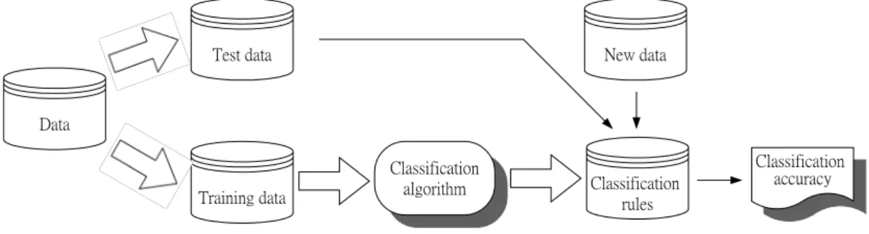
(10) Chapter 1. Introduction. 1.1.. Research Background. Learning is an essential component of any intelligent system, whether human, animal, or machine. Without learning, systems are unable to profit from their experience or to adapt to changing conditions. Simply recording experiences is usually not sufficient, as subsequent experiences may differ slightly and so any direct association between the experience and the effect may not be of any use.. Machine learning is an area of artificial intelligence involving developing techniques to allow computers to “learn.” More specifically, machine learning is a method for creating computer programs by the analysis of data sets, rather than the intuition of engineers. These systems often generate knowledge in the form of decision trees [1], [2] which are able to solve difficult problems of practical importance.. Machine learning is a two-step process, which finds the common properties among a set of examples in a database and classifies them into different classes, according to a classification model as shown in Fig. 1.1. In the first step, training data are analyzed by classification algorithm then it is represented in the form of classification rules, decision tree, or mathematical formulae. In the second step, testing data are used to estimate the accuracy of the classification rules. If the accuracy is considered acceptable, the rules can be applied to the classification of new. 1.

(11) data examples for which the class label is not known.. Test data. New data. Data. Training data. Fig. 1.1.. Classification algorithm. Classification rules. Classification accuracy. The machine learning process.. Machine learning algorithms can be categorized in several ways. Most importantly they are divided into supervised and unsupervised algorithms [3]. The supervised learning algorithm is told to which class each training example belongs. In case where there is no a priori knowledge of classes, supervised learning can be still applied if the data has a natural cluster structure. Then a clustering algorithm [3] has to be run first to reveal these natural groupings. In unsupervised learning, the system learns the classes on its own. This type of learning learns the classification by searching trough common properties of the data.. There are many ways to acquire automatically knowledge. Decision tree induction has been widely used in extracting knowledge from feature-based examples for classification. A decision tree based classification method is a supervised learning method that constructs decision trees from a set of examples. The quality of a tree depends on both the classification accuracy and the size of the tree. One of the most significant developments in the fundamental decision three algorithms is the ID3 algorithm, which is a popular and efficient method of making a decision tree for classification from discrete data without much computation. 2.

(12) ID3 stands for “Iterative Dichotomizer (version) 3,” and is a decision tree induction algorithm, developed by Quinlan [4], and later versions include C4.5 [5] and C5.0 [6]. In the ID3 approach, we make use of the labeled examples and determine how features might be examined in sequence until all the labeled examples have been classified correctly. But, there exist two major difficulties in ID3 algorithm.. 1). ID3 requires features to have discrete values, so it is not able to deal with continuous data, which serious limits the range of its applications.. 2). ID3 algorithm is suitable for crisp partition. In order to obtain fuzzy partition, the result needs to be fuzzified.. ID3 algorithm does not directly deal with continuous data. If the attributes are continuous, the algorithms must be integrated with a discretization algorithm [7], [8] that transforms them into several intervals, but these decision trees are not easy to understand. Furthermore, most knowledge associated with human’s thinking and perception has imprecision and uncertainty. On the basis of the above description, the fuzzy version of ID3 based on minimum fuzzy entropy was proposed. Investigations to fuzzy ID3 could be found in [1] and [9]–[17].. 1.2.. Motivation. Umano [9] and Janikow [1] have proposed Fuzzy ID3 algorithm which is tightly connected with characteristic features of the ID3 algorithm and is extended to apply to fuzzy sets of attributes and generates a fuzzy decision tree using fuzzy sets defined by a user for continuous attributes. For feature ranking, ID3 algorithm selects the feature based on the maximum information gain, which is computed by the probability of 3.

(13) training data, but Fuzzy ID3 by the probability of membership values for the training data.. Fuzzy ID3 is a typical algorithm of fuzzy decision tree induction, and from Fuzzy ID3, one can extract a set of fuzzy rules, which possess many advantage such as simplicity of the rules, moderate computational effort, and easy manipulation of fuzzy reasoning. But Fuzzy ID3 algorithm can only deal with continuous data and it is often criticized to result in poor learning accuracy.. In this thesis, we propose an algorithm to generate a fuzzy decision tree, which can accept continuous, discrete, or mixed-mode data sets [7], [8] using fuzzy sets and it is tuned by genetic algorithm [18]. Furthermore, we propose a method to prune the rule-base and re-tune the fuzzy sets again to improve the accuracy still by genetic algorithm. We can directly classify mixed-mode data by our proposed fuzzy ID3 schemes and achieves high accuracy rate due to the genetic tuning algorithm. For many famous data sets, we use the two-fold cross-validation procedure to estimate the classification accuracy. Finally, we analyze a website log-file data set using our algorithm to acquire effective rule that helps web master maintain and improve the website.. 1.3.. Thesis Outline. The organization of this thesis is structured as follows. Chapter 1 introduces the role of machine learning and the motivation of this research is explained. In Chapter 2, the attribute types will first be described. Then we introduce genetic algorithm based fuzzy ID3 method for mixed-mode attributes learning problem, and give an example 4.

(14) for comprehensibility. Chapter 3 describes the web log-file mining system, which consists of data-preparation engine, classification algorithm, and data analysis. The data preparation engine is designed for data clearing and removes all of redundancy in log-file database. Then genetic algorithm based fuzzy ID3 method is used to classify the web log-file. The data analysis is to summarize the database via a set of fuzzy rules found. For Chapter 4, the experiment of computer simulations on some famous data sets and web-log file are conducted and compared to C5.0. Finally, conclusion is presented in Chapter 5.. 5.

(15) Chapter 2. Genetic Algorithm Based Fuzzy ID3 Method. 2.1. Mixed-Mode Attributes Learning. An example is characterized by a set of attributes. The values of these attributes can be categorized roughly in two types:. 1). Continuous attribute: Continuous attributes have a proximity relation between them. For example, a man with height 7 feet is closely related to another person whose height is 6 feet 11 inches. So for continuous attributes, we can extract some relationship between the examples by analyzing their distances.. 2). Discrete attributes: Discrete attributes are nonnumeric and are unsuitable for proximity distance based analysis. For example, a man’s occupation is teacher, public servant or engineer that cannot be instead of ordinal number here.. All operands are considered continuous in our implementation. There are two ways to perform numerization of discrete attributes [19]. One method is to map the values of a discrete attribute to integers, so that the attribute can be considered as continuous inside our method. For example, if an attribute can take three possible values, then these discrete values are mapped into a set of integers, i.e., {0, 1, 2}. The disadvantage of this approach, however, lies in the fact that it imposes an order that does not exist in the original data. Another method is to divide a discrete attribute into. 6.

(16) n binary attributes, which is called “binarization,” if there are n possible values. (here, n > 2 ), with 0/1 representing the absence/presence of each value. This method overcomes the shortcomings of the first-integer approach, but will generate a large set of derived attributes if n is large. In this thesis, we use the binarization approach.. Our algorithm is designed to handle both continuous and discrete attributes. It combines the methods of ID3 [4] and fuzzy ID3 [9]. In other words, we can say that ID3 is a special case of our proposed Fuzzy ID3. In the traditional fuzzy ID3 algorithm, the fuzzy sets of all continuous attributes and the threshold values of leaf condition are user defined. But we cannot easily obtain the best solution of these parameters. Choosing these parameters is a decisive factor for good classification performance. In this thesis, we introduce genetic algorithm [18] to find out an optimal solution of the parameters of fuzzy ID3 algorithm that would greatly improve the learning accuracy of the decision tree. But the discrete attributes are divided into crisp sets, thus they have no membership functions. When deal with discrete attributes, our method is similarly to ID3. The details are described in the following sections.. 2.2. Feature Ranking. The order of features to construct the decision tree is an important issue to be investigated. The process to decide the order of features is called the Feature Ranking problem [9], [20], [21]. The feature ranking step is optional as we can use any arbitrary order of the features, but it is an important step because it will determine the size of the tree. With a good feature ranking, important features will be considered in the higher levels of the tree and can construct the decision tree in an efficient and accurate manners. 7.

(17) In fuzzy ID3 algorithm, we assign each example a unit membership value. Assume that we have a training set D , where each example has l continuous features A1, A2, ..., Al and n decision classes C1, C2, ..., Cn and m fuzzy sets Fi1, Fi2, ..., Fim for the feature Ai . Let DCk to be a fuzzy subset in D whose decision class is C k and |D| the sum of the membership values in a fuzzy set of data D .. The information gain G(Ai, D) for the attribute Ai by a fuzzy set of data D is defined by G(Ai, D) = I(D) à E(Ai, D) .. (2.1). For the training set, class membership is known for all the examples. Therefore, the initial entropy for the system consisting of membership values of D labeled examples can be expressed as I(D) = à. where. m P. k=1. (pk á log2 pk) ,. (2.2). C. |D k| pk = . |D|. (2.3). Weighting the entropy of each branch by its population can be written as. E(Ai, D) =. m P. (pij á I(DFij)) ,. (2.4). .. (2.5). j=1. where. pij =. |DFij|. m P. j=1. |DFij|. We will calculate the information gains G(Ai, D) and decide the order of features from the top to the bottom by decreasing G(Ai, D) gradually.. 8.

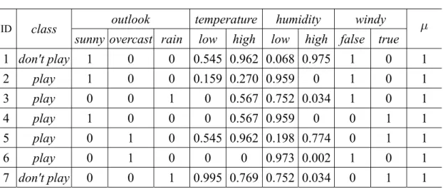
(18) Now, we will make use of a small training set to illustrate our learning process. The small training set is shown in Table I. The data set is a mixed-mode data [7], [8], and there are four attributes, namely outlook, temperature, humidity, and wind. The decision classes are don't play golf and play golf. In this example, the fuzzy sets of the continuous attributes are defined by genetic algorithm [18] that we will describe in the following section. The small training set with fuzzy representation is shown in Table II.. TABLE I A SMALL TRAINING SET windy. ö. 95. false. 1. 69. 70. false. 1. rain. 75. 80. false. 1. play. sunny. 75. 70. true. 1. 5. play. overcast. 72. 90. true. 1. 6. play. overcast. 81. 75. false. 1. 7. don't play. rain. 71. 80. true. 1. ID. class. outlook. temperature humidity. 1. don't play. sunny. 72. 2. play. sunny. 3. play. 4. TABLE II A SMALL TRAINING SET WITH FUZZY REPRESENTATION ID. class. outlook. temperature. sunny overcast rain. low. high. humidity low. windy. high false. true. ö. 1 don't play. 1. 0. 0. 0.545 0.962 0.068 0.975. 1. 0. 1. 2. play. 1. 0. 0. 0.159 0.270 0.959. 1. 0. 1. 3. play. 0. 0. 1. 0. 0.567 0.752 0.034. 1. 0. 1. 4. play. 1. 0. 0. 0. 0.567 0.959. 0. 1. 1. 5. play. 0. 1. 0. 0. 1. 1. 6. play. 0. 1. 0. 0.973 0.002. 1. 0. 1. 0. 0. 1. 0.995 0.769 0.752 0.034. 0. 1. 1. 7 don't play. 0 0. 0.545 0.962 0.198 0.774 0. 0. 9.

(19) Since we have |D| = 7, |DCdon0t play| = 2 and |DCplay| = 5, we have. I(D) ＝ −. 5 2 5 2 log 2 − log 2 7 7 7 7. ＝0.8631.. For outlook, we have 0. t play | = 1, |Dplay | = 2, |D outlook,sunny | = 3, |Ddon outlook,sunny outlook,sunny. and I(D outlook,sunny ) = 0.9183; 0. t play | = 0, |Dplay | = 2, |D outlook,overcast| = 2, |Ddon outlook,overcast outlook,overcast. and I(D outlook,overcast) = 0; 0. t play | = 1, |Dplay | = 1, |Doutlook,rain| = 2, |Ddon outlook,rain outlook,rain. and I(Doutlook,rain) = 1. Now we can calculate the expected information after testing by the outlook as 3 2 2 E(outlook, D) = × 0.9183 + × 0 + × 1 7 7 7 ＝0.6793.. For temperature, we have 0. don t play | = 1.54, |Dplay | = 0.704, |D temperature,low | = 2.244, |Dtemperature,low temperature,low. and I(D temperature,low ) = 0.8974; 0. don t play | = 1.731, |Dplay | = 2.366, |D temperature,high | = 4.097, |Dtemperature,high temperature,high. and I(D temperature,high ) = 0.9826;. E(temperature, D) = 0.9524. For humidity, we have 0. don t play | = 0.82, |Dplay | = 3.841, |D humidity,low | = 4.661, |Dhumidity,low humidity,low. and I(D humidity,low ) = 0.6711; 0. t play | = 1.009, |Dplay | = 0.81, |D humidity,high | = 1.819, |Ddon humidity,high humidity,high. 10.

(20) and I(D humidity,high ) = 0.9913;. E(humidity, D) = 0.7610. For windy, we have 0. t play | = 1, |Dplay | = 3, |D windy,false| = 4, |Ddon windy,false windy,false. and I(Dwindy,false) = 0.8113; 0. t play | = 1, |Dplay | = 2, |D windy,true| = 3, |Ddon windy,true windy,true. and I(Dwindy,true) = 0.9183;. E(windy, D) = 0.8572. Thus we have the information gain for the attribute outlook as. G(outlook, D) = I(D) à E(outlook, D) ＝0.8631－0.6793 ＝0.1838.. By similar analysis for temperature, humidity and windy, we have. G(temperature, D) = －0.0893, G(humidity, D) = 0.1021, and G(windy, D) = 0.0059.. Now we assign the order of features from the top to bottom by decreasing G(Ai, D) gradually. Then the order of features is {outlook, humidity, windy, temperature}.. 2.3. Tree Construction. Here the algorithm to generate a fuzzy decision tree [1], [2] is shown in the following:. 11.

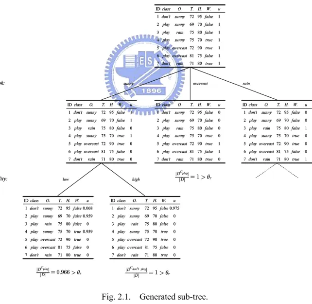
(21) 1). Generate the root node and select the most important feature by the result of feature ranking. Let all examples with the membership value 1.. 2). If a node t with a fuzzy set of data D satisfies the following conditions: ( 1 ) The proportion of a data set of a class C k is greater than or equal to a threshold òr , that is, C. |D k| õ òr , |D|. (2.6). ( 2 ) The number of a data set is less than a threshold òn , that is, . |D | < òn ,. (2.7). ( 3 ) There are no attributes for more classifications, C. |D k| then it is a leaf node, and we record the certainties of the node. |D| 3). If it does not satisfy the above conditions, it is not a leaf node, and the branch node is generated as follows: 3.1 ) Divide D into fuzzy subsets D1, D2, ..., Dm according to the feature Ai that will generate son nodes, where the membership value of example in D j is the product of the membership value in. D and the value of Fij of the value of Ai in D . 3.2 ) Generate. new. node. t1, t2, ..., tm. for. fuzzy. subsets. D1, D2, ..., Dm and label the fuzzy sets Fij to edges that connect between the nodes tj and t . 3.3 ) Select the next feature for generating the son nodes by the result of feature ranking. 4). Replace D by D j ( j ＝1, 2,…, m ) and repeat from step 2 ) recursively until the destination of all path are leaf nodes.. 12.

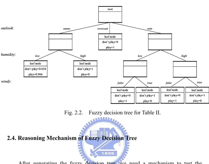
(22) In general, for continuous attributes, the number of linguistic terms is equal the number of the classes. To improve the accuracy, we can increase the number of linguistic terms for attributes and tuning the membership functions of these terms, but that will result in the increase of the number of extracted fuzzy rules. Now we have a part of decision tree as shown in Fig. 2.1. We apply the same process to construct decision tree until it hold the leaf conditions (1), (2), and (3) in the step 2 ) of the algorithm. For this data, we have the fuzzy decision tree as shown in Fig. 2.2.. outlook:. ID class. O.. 1 don't. sunny. O.. T.. H.. W.. W.. 2 play. sunny. 69 70 false. 1. rain. 75 80 false. 1. 4 play. sunny. 75 70 true. 1. 5 play overcast 72 90 true. 1. 6 play overcast 81 75 false. 1. 7 don't. 1. rain. 71 80 true. overcast. u. ID class. O.. 1 don't sunny. 72 95 false. 1. 1 don't. sunny. T. H.. W.. 2 play. sunny. 69 70 false. 1. 2 play. sunny. 69 70 false. 3 play. rain. 75 80 false. 0. 3 play. rain. 75 80 false. 4 play. sunny. 75 70 true. 1. 4 play. sunny. 75 70 true. 5 play overcast 72 90 true. 0. 5 play overcast 72 90 true. 72 95 false. O.. 1 don't. sunny. 2 play. sunny rain. 4 play. sunny. sunny. T. H.. W.. 0. 2 play. sunny. 69 70 false. 0. 0. 3 play. rain. 75 80 false. 1. 0. 4 play. sunny. 75 70 true. 0. 1. 5 play overcast 72 90 true. 0. 72 95 false. u 0. 6 play overcast 81 75 false. 1. 6 play overcast 81 75 false. 0. 7 don't. 0. 7 don't. 1. 71 80 true. rain |D play| |D|. high. W.. u. ID class. O.. T.. H.. W.. 71 80 true. 1 don't sunny. 72 95 false 0.975. 69 70 false 0.959. 2 play. sunny. 69 70 false. 75 80 false. 3 play. rain. 75 80 false. 0. 4 play. sunny. 75 70 true. 0. 0. 75 70 true 0.959. 0. 0. 5 play overcast 72 90 true. 0. 0. 6 play overcast 81 75 false. 0. 7 don't. 0. 7 don't. 0. 71 80 true. C. = 0.966 > òr. rain. 71 80 true. C don0t play |. |D. |D|. = 1 > òr. u. 72 95 false 0.068. 5 play overcast 72 90 true. |D play| |D|. O.. 1 don't. 0. rain. 6 play overcast 81 75 false rain. ID class. 0. T. H.. 3 play. u 0. 6 play overcast 81 75 false. low. ID class. rain. 7 don't. C. humidity:. u 1. 3 play. sunny. ID class. T. H.. 72 95 false. = 1 > òr. Fig. 2.1. Generated sub-tree.. 13. rain. 71 80 true.

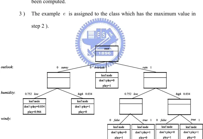
(23) root. outlook:. sunny. overcast. rain. leaf node don’t play=0 play=1. humidity:. low. high. leaf node. leaf node. don’t play=0.034. don’t play=1. play=0.966. play=0. low. windy:. false. high. true. true. false. leaf node. leaf node. leaf node. leaf node. don’t play=0. don’t play=1. don’t play=0. don’t play=1. play=1. play=0. play=1. play=0. Fig. 2.2. Fuzzy decision tree for Table II.. 2.4. Reasoning Mechanism of Fuzzy Decision Tree. After generating the fuzzy decision tree, we need a mechanism to test the classification of training examples or to predict the classification of novel examples. C. |D k| At all the leaf nodes, we have recorded the certainties of each class , then the |D|. reasoning by fuzzy decision tree can be converted into that by a set of fuzzy rules. For example, the fuzzy rule extracted from this node can be describe as. IF outlook is sunny AND humidity is low THEN don’t play with certainty 0.034 and play with certainty 0.966.. For a generated fuzzy decision tree, each connection from root to leaf is called a path. There are one or more membership values on a path, because a continuous. 14.

(24) attribute value has a membership value according to the corresponding membership function. Assume that the generated fuzzy decision tree contains r leaf nodes, and n decision class. A mechanism commonly used for determining the example e is described as follows:. 1). For each i ( 1 ô i ô r ), the certainty of class j of the leaf node i multiplied by the membership values which are on the path i . Sum the r terms to get P(j) which is the possibility of the class j .. 2). Repeat from step 1 ) for each j ( 1 ô j ô n ) such that all the P(j) have been computed.. 3). The example e is assigned to the class which has the maximum value in step 2 ).. root. outlook:. 0. sunny. 0. overcast. rain 1. leaf node don’t play=0 play=1. humidity:. 0.752 low. high 0.034. leaf node. leaf node. don’t play=0.034. don’t play=1. play=0.966. play=0. 0.752 low. windy:. 0 false. high 0.034. true 1. 0 false. true 1. leaf node. leaf node. leaf node. leaf node. don’t play=0. don’t play=1. don’t play=0. don’t play=1. play=1. play=0. play=1. play=0. Fig. 2.3. Fuzzy reasoning in fuzzy decision tree.. An illustration is shown in Fig. 2.3, where the 7-th example of Table I been tested by the rule-base. Thus we can use these 7 rules to classify the 7-th example of Table I as follows: 15.

(25) P(don0t play) = 0×0.752×0.034 + 0×0.034×1 + 0×0 + 1×0.752×0×0 + 1×0.752×1×1 + 1×0.034× 0×0 + 1×0.034×1×1 = 0.7860,. P(play) = 0×0.752×0.966 + 0×0.034×0 + 0×1 + 1×0.752×0×1 + 1×0.752×1×0 + 1×0.034× 0×1 + 1×0.034×1×0 = 0.. The 7-th example is assigned to class don’t play because P(don0t play) is the maximum. Note that we use all rules to classify an example but not just depend on a single rule.. 2.5. Genetic Algorithm for Fuzzy ID3 Method. From the description above, ò r, ò n , and the membership functions of all the continuous features of Fuzzy ID3 algorithm are defined by a user. A good selection of fuzzy rule-base, òr, òn , and the membership functions are best matched to the database to be processed, would greatly improve the accuracy of the decision tree. To this end, any optimization algorithms seem appropriate for this purpose. In particular, genetic algorithm (GA) based scheme is highly recommended since a gradient computation for conventional optimization approach is usually not feasible for a decision tree. This is because condition-based decision path is nonlinear in nature, and hence its gradient is not defined. Now we will introduce GA to search best ò r, ò n , and the membership functions of all the continuous features for the design of Fuzzy ID3. 16.

(26) GA is adaptive heuristic search method that may be used to solve all kinds of complex search and optimization problems. GA is based on the evolutionary ideas of natural selection and genetic processes of biological organisms. As the natural populations evolve according to the principles of natural selection and “survival of the fittest,” first laid down by Darwin, so by simulating this process, GA is able to evolve solutions to real-world problems, if it has been suitably encoded. GA is often capable of finding optimal solutions even in the most complex of search spaces or at least it offers significant benefits over other search and optimization techniques. A typical GA operates on a population of solutions within the search space. The search space represents all the possible solutions that can be obtained for the given problem and is usually very complex or even infinite. Every point of the search space is one of the possible solutions and therefore the aim of the GA is to find an optimal point or at least come as close to it as possible.. GA is typically implemented as a computer simulation in which a population of chromosomes of individuals to an optimization problem evolves toward better solutions. Traditionally, solutions are represented in binary as strings of 0s and 1s, but different encodings are also possible. In this thesis, we use 6-bits to represent a parameter. The membership function of each sub-attribute is assumed to be Gaussian-type and given by m(x) = exp (à. (xàö)2 ) 2û2 ,. (2.8). where x is the corresponding feature value of the example with mean ö and standard deviation û . Thus for each membership function, we have two parameters. ö and û to tune.. 17.

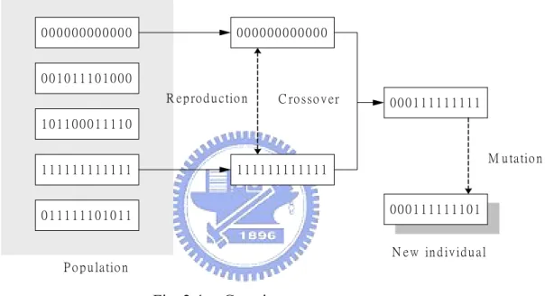
(27) For example, assume we have a data set, which has 4 continuous attributes and 3 classes such that there are 12 membership functions. Each membership function has 2 parameters and there are 2 thresholds of leaf condition in addition. Thus we have 26 parameters to be tuned, and the length of a binary chromosome is 156. The GA consists of three genetic operators: reproduction, crossover, and mutation as shown in Fig. 2.4.. 000000000000. 000000000000. 001011101000. R e p ro d u c tio n. C ro sso v e r. 000111111111. 101100011110. 111111111111. M u ta tio n. 111111111111. 000111111101. 011111101011. N e w in d iv id u a l P o p u la tio n. Fig. 2.4. Genetic operators.. Reproduction is a process in which potential chromosomes (chromosomes with higher fitness value) of the population are copied into a mating pool depending on their fitness function values. To minimize the rule number and maximize the accuracy, let the fitness function f = 100((100(Ai à Aworst))2/100 + (Ravg/Ri )) ,. (2.9). where Ai is the learning accuracy of the individual i , and Aworst is the worst learning accuracy of all individuals. R avg is the average number of the rules of all individuals, and Ri is the number of the rules of the individual i .. 18.

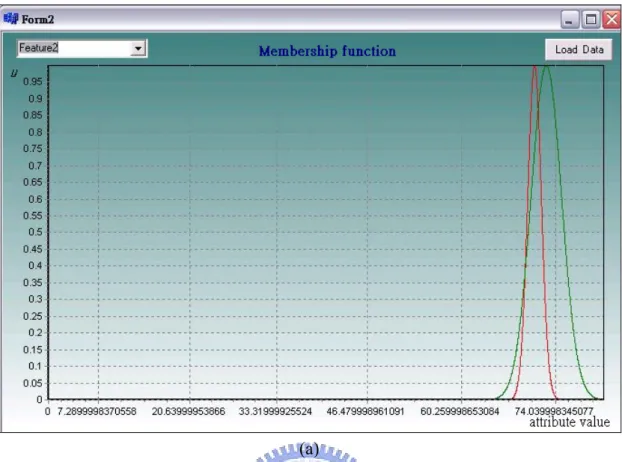
(28) Crossover operation produces offspring by exchanging information between two potential chromosomes selected randomly from the mating pool generated by the reproduction process. For example, consider two chromosomes a = 000000000000 and b = 111111111111 of length 12 selected randomly from the mating pool. A random position 3 is selected for crossing over. After crossover, the two chromosomes are a = 000111111111 and b = 111000000000.. Mutation is an occasional alteration of a random bit. A random bit of a randomly selected chromosome in the population is selected and the bit value is reversed. For example, consider a chromosome a = 000111111111 of length 12 generated by crossover process. A random bit 11 is selected for mutating. After mutation, the chromosome is a = 000111111101. Mutation that helps to find an optimal solution to the given problem more reliably, as it prevents GA from finishing the search prematurely with a sub-optimal solution.. After GA, the system will generate Gaussian-type membership functions base on ö and û , which represent mean and variance respectively. The membership functions of each attribute for the small training set as shown in Table I are illustrated in Fig. 2.5, and we get òr = 7.4286 â 10à1 , and òn = 1.0000 â 10à3 . Note that the discrete attributes have no membership functions. Fig. 2.6 gives a schematic description of the basic structure of GA.. 19.

(29) (a). (b) Fig. 2.5. The membership functions of each attribute for the small training set. (a) The membership functions of temperature. (b) The membership functions of humidity.. 20.

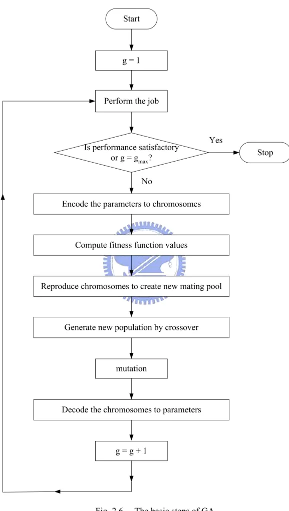
(30) Start. g=1. Perform the job. Is performance satisfactory or g = gmax?. Yes. No Encode the parameters to chromosomes. Compute fitness function values. Reproduce chromosomes to create new mating pool. Generate new population by crossover. mutation. Decode the chromosomes to parameters. g=g+1. Fig. 2.6. The basic steps of GA. 21. Stop.

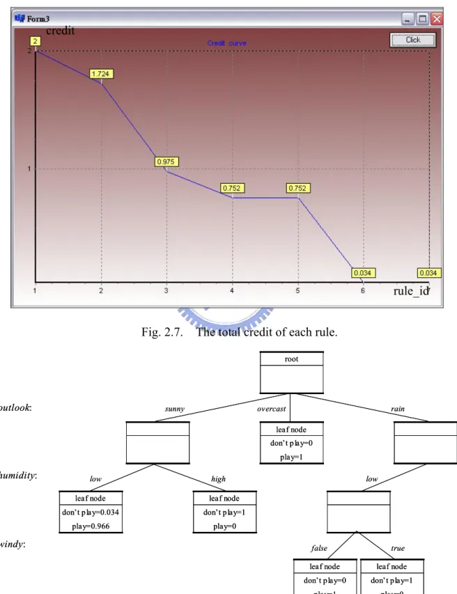
(31) 2.6. Rule Pruning. We have used GA to improve the accuracy of the classification task and decrease the rule number as well. But it is possible that there are still some redundant rules in our rule-base. Thus, a simple but effective scheme for rule minimization is described as follows:. 1 ) When an example is classified, we maintain the production value of the membership values and the certainty of each class. For example, Pi( j) is represented that the possibility of the class j estimated by the rule i . 2 ) For each j ( 1 ô j ô n ), Pi( j) corresponding to the correct class label of the example gets positive sign and others get negative sign. For example, if the example is class 1 such as Pi(1) is positive and others ( Pi(2), …) are negative. 3 ) Sum the possibilities of all the classes estimated by the rule i ( Pi(1) ,. Pi(2), …) then we get the credit of the rule i for classifying this example. 4 ) Consider the next test example and repeat from step 1 ) until all the test examples are estimated by rule i and we will get the total credit of rule i . 5 ) Repeat from step 1 ) for each i ( 1 ô i ô r ) such that the total credit of all the rules have been computed. 6 ) Remove the redundant rules whose total credit is less than a threshold.. For example, after we getting the total credit of each rule of the small training set as shown in Table I, we sort and plot the total credit of all rules as shown in Fig. 2.7. We find that after about the 5-th rule, the slope takes a sudden turn and slides down rapidly. It means that the 6-th and 7-th rules may be bad or redundant rules. Hence we 22.

(32) can select a threshold between 0.034 and 0.752 then the redundant rules would be removed. The Pruned fuzzy decision tree of the small training set as shown in Table I is shown in Fig. 2.8, and the entire process of our method is schematized in Fig. 2.9.. credit. rule_id Fig. 2.7. The total credit of each rule. root. outlook:. sunny. overcast. rain. leaf node don’t play=0 play=1. humidity:. low. high. leaf node. leaf node. don’t play=0.034. don’t play=1. play=0.966. play=0. windy:. low. false. leaf node. leaf node. don’t play=0. don’t play=1. play=1. play=0. Fig. 2.8. Pruned fuzzy decision tree. 23. true.

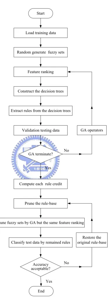
(33) Start. Load training data. Random generate fuzzy sets. Feature ranking. Construct the decision trees. Extract rules from the decision trees. GA operators. Validation testing data. GA terminate?. No. Yes. Compute each rule credit. Prune the rule-base. Tune fuzzy sets by GA but the same feature ranking. Classify test data by remained rules. Accuracy acceptable?. Restore the original rule-base. No. Yes End. Fig. 2.9. Steps in GA based fuzzy ID3 method. 24.

(34) Chapter 3. Web Log-File Classification. 3.1. Introduction to Web-Mining. In the past ten years, the internet has changed a lot, and becomes close related to our daily life. According to the need of human being, the model of internet is more and more completed. Through the internet, people can get any information from the website, and exchange mutual information via internet. Because of convenience and unlimited cyberspace properties, the internet create a new business model “e-commerce” that changed the traditional business model. If people want to buy or sell something through internet, they can get information on virtual website and need not any actual store. It is an initiative to change the traditional business world. When people connect to website, the web server would record IP of the user, the background of the user, visited web pages, visited time, etc. in its log-file. The format of log-file is detailed specification of W3C referred in [22] and [23]. The web server kept of all consumers’ transactions and records. Hence, the log-file becomes very large through day’s recording day in day out. How to extract important regularity or domain knowledge hidden behind the log-file is important to the enterprise for improving their content services to the potential users.. 3.2. Data Preparation. The data mining system [3] is to extract efficient information form web log-file. We have to transfer the original log-file to some special format suitable for the. 25.

(35) database in this system. We selected the Microsoft Access 2000, a relational database, to be the log-file database format. When converted the log-file from text file to Access database file, the attributes (fields) of log-file must be defined. The definition of fields are shown as follows:. from_ip: where the consumer came from. date: the date that consumer login website. time: the time that consumer login website. status: the HTTP status code returned to the client. dest: the hyperlinks that consumer clicked.. After the converting above, Fig. 3.1 is the log-file table. The consumer table is the basic characteristics of members of the website. The definition of fields in the consumer table are shown as follows:. fromip: the IP of the consumer. name: the consumer’s name. sex: the sex of the consumer. age: the age of the consumer. education: the education level of the consumer. occupation: the occupation of the consumer. income: the total income in a year.. Fig. 3.2 is the table of consumers. The log-file table and the consumer table are two important elements of web log-file mining system. The consumer table provides the basic personal information about a consumer. The log-file table registers the in 26.

(36) and out of website’s pages, whose records will be utilized for analysis later.. Fig. 3.1.. Fig. 3.2.. The log-file table.. The consumer table. 27.

(37) Web server will record the hyperlink pages that a consumer clicked. According to the hyperlink pages we get six categories of products that include books, compact disk (CD), computer, mobile, PDA, and electric commerce (EC). The metadata table as shown in Fig. 3.3 provided the numeric of hyperlink pages.. Because the log-file data may be in a mess with useful and non-useful data, we cannot use them in data mining algorithm directly. We will take out useful data by transferring it to particular format according to database setting beforehand, and clean out non-useful data. The major purpose of data cleaning is to reduce the redundancy of log-file and to convert the text file into Access database type. Therefore, the standard query language (SQL) can be applied to maintain the log-file database, such as query, insert, update, and delete.. Compare the log-file table with the consumer table and find out the consumer’s personal data such as sex, age,…, etc. Then 2604 examples of the web log-file data will be generated, and as shown in Fig. 3.4. The web log-file data stores records consisted of the log-file, consumer, and metadata tables, and the internal data may be discrete or continuous data. To analyze the web log-file, the training sample table is very important. It provides the information about the consumers’ sex, age, education level, occupation, and total income in one year. It also provides consumers’ spending time and favorite pages. The training samples table also helps us to explain the behavior of consumers. Through the fuzzy sets of values of linguistic variable, GA based fuzzy ID3 method will generate fuzzy inference rules.. 28.

(38) Fig. 3.3.. Fig. 3.4.. The metadata table.. The web log-file data. 29.

(39) 3.3. Data Analysis. The web log-file data with 2604 examples has six attributes and six classes named books (class 1), CD (class 2), computer (class 3), mobile (class 4), PDA (class 5), and EC (class 6). There are two continuous attributes, and four discrete attributes, as shown in Table III.. The class distribution of the web log-file data is shown in Fig. 3.5. The highest proportion of the classes is “Books” (44%), and the lowest is “EC” (nearly 0%). Now, we make the statistics of the repeated numbers of each example and the class distribution of the examples as shown in Fig. 3.6. For example, the 14-th example is the same with the 6-th example, and there are nine examples in the training data the same with this example. Among the nine examples, there are three class 1, three class 3, and three class 5. The probability of class 1 of the nine examples is 0.33. The probability of each class is shown in Fig. 3.7.. TABLE III DETAILS OF THE ATTRIBUTES Type. Attribute. Attribute range. Age (years old) {15 - 41} Continuous Spend time. {0.002227 - 1}. Sex. {Man, Woman}. Education. {Below junior, Junior, Senior, University, MS/PHD}. Occupation. {Student, Public, Finance, Service, Information}. Income. {Below 20K, 20K-40K, 40K-60K, 60K-80K, 80K-100K}. Discrete. 30.

(40) Fig. 3.5.. The class distribution of the web log-file data.. Fig. 3.6.. Statistical analysis of the data repeated.. 31.

(41) Fig. 3.7.. The probability of each class.. The web log-file data is not in good order because that there exist some people with all the same attributes but their favorites are different. This case always exists in the real world. In the testing process, we can predict only one class for each input example. In this data set, we always have some examples that will not be correctly classified, assume a classification of majority class. If we want to distinguish the repeated example clearly, we will need to add another attributes if possible. But it is limited in source acquired of the data. For example, there are ten examples with all the same attributes, that seven examples are in class 1 and three examples are in class 2. If the classified results of the ten examples are class 1, the accuracy will be 70%. Inevitably there are three examples classified wrongly. Thus our purpose is to find the regularity of the most important ones, i.e., fist choice. We will provide information 32.

(42) about the behavior of the user through the fuzzy ID3 method, and the rule-base obtained has to be simple and efficient.. 33.

(43) Chapter 4. Simulation and Experiment. As mentioned in Chapter 2, we introduce fuzzy ID3 algorithm, whose membership functions and leaf condition are tuned by GA. In this chapter, we apply the algorithm to classify some data sets, which include continuous, discrete, and mixed-mode data sets [7], [8]. Finally, we used a daily log-file to analysis and generated the rule-base about consumer behavior to web master to maintain and promote the website content.. 4.1. The Data Sets. The ten data sets employed for experiments are obtained from the University of California, Irvine, Repository of Machine Learning databases (UCI) [24]. Their characters are briefly described below and summarized in Table IV.. 1). Crude_oil: Gerrid and Lantz analyzed Crude_oil samples from three zones of sandstone. The Crude_oil data set with 56 examples has five attributes and three classes named wilhelm, submuilinia, and upper. The attributes are vanadium (in percent ash), iron (in percent ash), beryllium (in percent ash), saturated hydrocarbons (in percent area), and aromatic hydrocarbons (in percent area).. 2). Glass Identification Database: The data set represents the problem of identifying glass samples taken from the scene of an accident. The 214 examples were originally collected by B. German of the Home Office. 34.

(44) Forensic Science Service at Aldermaston, Reading, Berkshire in the UK. The nine attributes are all real valued and fully known, representing refractive index and the percent weight of oxides such as silicon, sodium, and magnesium. The six classes are named as building windows float processed, building windows not float processed, vehicle windows float processed, containers, tableware, and headlamps. 3). Iris Plant Database: The Iris data set, Fisher’s classic test data (Fisher, 1936), has three classes with four-dimensional data consisting of 150 examples. The four attributes are: sepal length, sepal width, petal length, and petal width. This data set gives good results with almost all classic learning methods and has become a sort of benchmark data.. 4). Myo_electric: The Myo_electric data set is extracted from a problem in discriminating between electrical signals observed at the human skin surface. This is a four-dimensional data set consisting of 72 examples divided into two classes.. 5). Norm4: The data set has 800 examples consisting of 200 examples each from the four components of a mixture of four class 4-variate normals.. 6). BUPA liver disorders: This UCI data set was donated by R. S. Forsyth. The problem is to predict whether or not a male patient has a liver disorder based on blood tests and alcohol consumption. There are two classes, six continuous attributes, and 345 examples.. 7). Promoter Gene Sequences Database: Promoters have a region where a protein (RNA polymerase) must make contact and the helical DNA sequence must have a valid conformation so that the two pieces of the contact region spatially align. The data set with 106 examples has 57 attributes and two classes. All attributes are discrete. 35.

(45) 8). StatLog Project Heart Disease dataset: This UCI data set is from the Cleveland Clinic Foundation, courtesy of R. Detrano. The problem concerns the prediction of the presence or absence of heart disease given the results of various medical tests carried out on a patient. There are two classes, seven continuous attributes, six discrete attributes, and 270 examples.. 9). Golf: The data set with 28 examples has four attributes and two classes named play, and don’t play. There are 2 continuous and 2 discrete attributes. The attributes are outlook, temperature, humidity, and windy.. 10) StatLog Project Australian Credit Approval: This credit data originates from Quinlan. This file concerns credit card applications. All attribute names and values have been changed to meaningless symbols to protect confidentiality of the data. The Australian data set with 690 examples has 14 attributes and two classes. There are 6 continuous and 8 discrete attributes.. TABLE IV SUMMARY OF THE DATABASES EMPLOYED # of examples. # of attributes. # of continuous attributes. # of classes. Crude_oil. 56. 5. 5. 3. Glass. 214. 9. 9. 6. Iris. 150. 4. 4. 3. Myo_electric. 72. 4. 4. 2. Norm4. 800. 4. 4. 4. Bupa. 345. 6. 6. 2. Promoters. 106. 57. 0. 2. Heart. 270. 13. 6. 2. Golf. 28. 4. 2. 2. Australian. 690. 14. 6. 2. Data set. 36.

(46) 4.2. Comparison. The performance of our rule-base on the above data sets is shown in Table V. We use all the examples to be the training data and the same examples to be the testing data for performance evaluation. In rule pruning, we remove redundant rules that can keep or slightly reduce learning accuracy to be considered as acceptable. According to feature subset select [25], for classifying Glass data set, we consider only five attributes that are Na, Mg, Al, K, Ba. If we do not reduce the attributes of Glass data set, we will get more rules after tree construction, but it will not help in increasing the learning accuracy.. TABLE V PERFORMANCE OF THE RULE-BASE ON DIFFERENT DATA SETS Data set. Before rule pruning. After rule pruning. # of rules. Training acc.. # of rules. Training acc.. Crude_oil. 9.0. 100.0. 7.0. 98.2. Glass. 61.0. 77.6. 12.0. 76.2. Iris. 7.0. 99.3. 4.0. 98.7. Myo_electric. 4.0. 98.6. 2.0. 98.6. Norm4. 14.0. 97.0. 10.0. 96.8. Bupa. 15.0. 76.5. 11.0. 76.5. Promoters. 7.0. 85.9. 4.0. 85.9. Heart. 15.0. 87.4. 12.0. 85.9. Golf. 9.0. 100.0. 7.0. 100.0. Australian. 5.0. 87.0. 4.0. 87.0. From Table V, we can find that for Myo_electric, Bupa, Promoters, Golf, and Australian data sets, the accuracy remains the same before and after rule pruning. For the others, there is a little degradation in accuracy. This has happened possibly 37.

(47) because the rule pruning process has removed some rules, which were correctly classifying a few examples and the residual rule-base is not able to correctly classify these examples. We can also see that the number of the rules is decreased for all data sets, which shows the effectiveness of our rule pruning process.. So far, we have not evaluated the generalization ability of the rules extracted by our scheme. Next, we do so and also compare our results with the outputs of C5.0 [6]. The reason why we choose C5.0 is that C5.0 worked well for many decision-making problems and it was a decent version of C4.5. We use that for each considered data set, 50% of the data is uniformly and randomly chosen as the training set and the remaining 50% of cases is held for testing. This procedure is repeated six times. Note that, C5.0, whose demonstration version is limited up to 400 examples, and free download from RuleQuest Research Data Mining Tools [6]. We use this demonstration version of C5.0 to construct the following tables.. Table VI shows the comparison of the accuracy of our rule-base and that from C5.0. It records the testing accuracy from two-fold cross validation repeated six times on each data set. On average, we find that our rule-base outperforms C5.0 in eight out of ten data sets. Thus our system has a better generalization ability than C5.0 and except for Glass and Bupa. The results of our rule-base and C5.0 were also compared with respect to their average numbers of rules. Table VII compares the numbers of rules generated by our rule-base and C5.0 at the same experiment on these data sets. We find that our rule-base outperforms C5.0 in five out of ten data sets. But, the total average number of the rules on our rule-base is 7.18, which less than 8.17 of C5.0. It is evident that our approach tends to produce more compact rule sets than C5.0.. 38.

(48) TABLE VI COMPARISON OF THE ACCURACY RATES Testing acc. (two-fold CV repeated six times) Data set. Avg.. Algorithm 1. 2. 3. 4. 5. 6. acc.. Our rule-base. 85.7. 87.5. 75.0. 83.9. 73.2. 82.1. 81.2*. C5.0. 76.8. 78.6. 80.4. 80.4. 76.8. 75.0. 78.0. Our rule-base. 64.0. 66.4. 65.4. 61.2. 64.0. 63.1. 64.0. C5.0. 65.9. 67.8. 65.0. 67.3. 66.4. 69.6. 67.0*. Our rule-base. 96.0. 93.3. 94.7. 96.0. 95.3. 94.0. 94.9*. C5.0. 92.0. 94.7. 92.0. 92.7. 91.3. 92.7. 92.6. Our rule-base. 81.9. 93.1. 83.3. 91.7. 91.7. 91.7. 88.9*. C5.0. 83.3. 90.3. 79.2. 86.1. 93.1. 88.9. 86.8. Our rule-base. 93.8. 94.4. 94.4. 95.3. 94.3. 92.5. 94.1*. C5.0. 89.8. 91.3. 91.3. 90.6. 91.8. 89.9. 90.8. Our rule-base. 60.9. 59.7. 64.6. 64.1. 64.4. 64.1. 63.0. C5.0. 65.8. 62.3. 65.8. 68.7. 63.5. 64.0. 65.0*. Our rule-base. 76.4. 76.4. 68.9. 76.4. 79.3. 75.5. 75.5*. C5.0. 75.5. 74.5. 69.8. 71.7. 78.3. 78.3. 74.7. Our rule-base. 76.7. 80.0. 77.4. 78.2. 78.2. 77.0. 77.9*. C5.0. 74.1. 77.0. 76.3. 77.8. 79.6. 73.3. 76.4. Our rule-base. 92.9. 67.9. 60.7. 85.7. 82.1. 78.6. 78.0*. C5.0. 82.1. 71.4. 57.1. 71.4. 78.6. 71.4. 72.0. Our rule-base. 84.6. 84.1. 85.5. 84.8. 84.4. 84.4. 84.6*. C5.0. 83.2. 84.5. 85.4. 85.8. 84.8. 83.1. 84.5. Crude_oil. Glass. Iris. Myo_electric. Norm4. Bupa. Promoters. Heart. Golf. Australian. 39.

(49) TABLE VII COMPARISON OF THE NUMBER OF THE RULES Data set. # of rules (two-fold CV repeated six times). Avg.. 1. 2. 3. 4. 5. 6. rules. Our rule-base. 5.5. 5.0. 5.5. 6.0. 5.0. 5.5. 5.4. C5.0. 4.0. 4.0. 5.0. 4.0. 4.5. 3.0. 4.1*. Our rule-base. 20.0. 12.5. 13.0. 15.0. 16.0. 9.0. 14.3. C5.0. 10.0. 9.5. 13.5. 7.0. 9.5. 9.0. 9.8*. Our rule-base. 4.5. 3.0. 4.5. 5.0. 5.0. 5.0. 4.5. C5.0. 4.0. 3.5. 3.0. 4.0. 3.0. 3.0. 3.4*. Our rule-base. 2.5. 2.5. 2.5. 3.5. 2.0. 3.5. 2.8*. C5.0. 3.5. 3.0. 3.5. 4.0. 3.5. 4.0. 3.6. Our rule-base. 12.0. 9.5. 17.0. 12.0. 13.0. 10.0. 12.3*. C5.0. 14.5. 14.5. 13.5. 12.5. 11.5. 14.5. 13.5. Our rule-base. 5.5. 5.0. 3.5. 7.0. 7.0. 4.0. 5.3*. C5.0. 14.0. 9.5. 17.0. 13.0. 16.0. 11.0. 13.4. Our rule-base. 5.0. 1.5. 3.5. 12.5. 8.0. 8.5. 6.5*. C5.0. 9.0. 7.0. 8.5. 8.0. 5.5. 7.5. 7.6. Our rule-base. 16.0. 9.5. 15.0. 14.0. 7.0. 13.5. 12.5. C5.0. 11.0. 12.0. 12.5. 11.5. 12.5. 11.5. 11.8*. Our rule-base. 5.0. 3.5. 4.5. 6.0. 5.5. 6.5. 5.2. C5.0. 5.0. 4.5. 2.5. 2.5. 3.0. 2.5. 3.3*. Our rule-base. 3.5. 3.0. 2.5. 2.0. 3.5. 3.5. 3.0*. C5.0. 8.5. 10.5. 13.5. 11.5. 14.0. 9.0. 11.2. Algorithm. Crude_oil. Glass. Iris. Myo_electric. Norm4. Bupa. Promoters. Heart. Golf. Australian. 40.

(50) TABLE. VIII. THE BEST PERFORMANCE COMPARISON Data set. Our rule-base # of rules. C5.0 rule-base. Training acc. Testing acc.. # of rules. Testing acc.. *. Crude_oil. 5.0. 100.0. 87.5. 4.0. 80.4. Glass. 12.5. 77.6. 66.4. 9.0. 69.6*. Iris. 4.5. 100.0. 96.0*. 3.5. 94.7. Myo_electric. 2.5. 97.2. 93.1. 3.5. 93.1. *. Norm4. 12.0. 96.0. 95.3. 11.5. 91.8. Bupa. 3.5. 72.5. 64.6. 13.0. 68.7*. Promoters. 8.0. 89.6. 79.3*. 5.5. 78.3. 85.2. *. 12.5. 79.6. *. Heart. 9.5. 80.0. Golf. 5.0. 100.0. 92.9. 5.0. 82.1. Australian. 2.5. 88.6. 85.5. 11.5. 85.8*. Table VIII lists the maximum testing accuracy of the six for our rule-base and C5.0 in Table VI. It also shows the corresponding number of the rules in the experiment. With respect to the testing accuracy shown in Table VIII, our rule-base is still superior to C5.0 in six data sets and ties one. The discrete attributes do not assume membership functions to be tuned by GA, the performance of the discrete and mixed-mode data sets are still better than C5.0.. 4.3. Classification of the Web Log-File. Now we will use our fuzzy ID3 method to find the regularity of the web log-file. The training data of this experiment was described in Chapter 3. After training, our method will generate a fuzzy decision tree and the membership functions of each continuous attribute. Through the fuzzy decision tree, we can extract a set of fuzzy rules. When testing, we use the fuzzy rule-base to classify all the examples in the log-file. 41.

(51) To validate the effectiveness of the rule set, we use all of the training data to be the testing data also. Our program interface is shown in Fig. 4.1. If the classifier is towards the majority class classification, the best accuracy we can have 58.99%. The learning accuracy is poor because of high inconsistency existing in the data set. In this data set, there exist some person with all the same attributes but their favorite classes are different. In fact, based on our proposed method, the majority class accuracy is 48.69% after training. The relative accuracy of the major class is 82.54%. The result of classifying is shown in Fig. 4.2. According to the rule credits as shown in Fig. 4.3, if the threshold to prune rule is chosen to be –10, there is only one redundant rule pruned in the rule-base. Then, the accuracy will be reduced to 47.35%. To maintain the accuracy we will not prune any rule in this experiment. Finally, the rule table is shown in Fig. 4.4, and the web master can maintain and improve the website according to these rules we have obtained.. Fig. 4.1.. Program interface.. 42.

(52) Fig. 4.2.. The result of classifying.. credit. rule_id Fig. 4.3.. The rule credits.. 43.

(53) 44. Fig. 4.4.. The rule table..

(54) There are 12 rules in the rule table, and the result of feature ranking is {Age, Spend time, Occupation, Income, Education, Sex}. The theorem of feature ranking was described in Chapter 2.2. We determine the order of the features to construct the decision tree by computing the entropy of the features. With feature ranking, important features will be considered in the higher levels of the tree and can construct the decision tree in an efficient and accurate manners. We utilize linguistic values to represent the attributes as shown in Table IX. Note that to acquire simple rules, we let the number of linguistic terms of the continuous attributes be 3, and the corresponding fuzzy sets are shown in Figs. 4.5–4.6. The rules can be very helpful to market analysis. For example, let us take the 7-th rule in Fig. 4.4, and the semantics of the rule is that:. IF the people is youth AND spends a little time in internet AND his occupation belongs to information industry THEN his favorite category of the products is Books with certainty 0.82 AND second favorite category of the products is PDA with certainty 0.18.. TABLE IX LINGUISTIC VALUES OF THE ATTRIBUTES Type. Attribute. Linguistic values. Age. {Youth, Middle age, Old}. Spend time. {Less, A little, More}. Sex. {Man, Woman}. Education. {Below junior, Junior, Senior, University, MS/PHD}. Occupation. {Student, Public, Finance, Service, Information}. Income. {Below 20K, 20K-40K, 40K-60K, 60K-80K, 80K-100K}. Continuous. Discrete. 45.

(55) ö Youth. Middle age. Old. attribute value Fig. 4.5.. ö. Less. The membership functions of Age.. A little. More. attribute value Fig. 4.6.. The membership functions of Spend time.. 46.

(56) Chapter 5. Conclusion. In this thesis, we have proposed an algorithm to generate a fuzzy decision tree, which can accept continuous, discrete, or mixed-mode data sets and it is tuned by genetic algorithm. Next, we propose a method to prune the rule-base and re-tune the feature’s membership functions again to improve the accuracy. The feature ranking remains unchanged before and after pruning. Our proposed method can directly classify mixed-mode data set and achieve high classification accuracy. We evaluated our method on several data sets, which include continuous, discrete, and mixed-mode data sets and consistently obtained very high accuracy rates with small number of rules. Finally, we analysis a web log-file data set using our method, and provide a set of rule-base to web master to improve the content of the website.. For continuous attributes, the learning accuracy of fuzzy decision tree is usually poor when the number of linguistic terms for attributes is very small. To improve the learning accuracy, we can increase the number of linguistic terms for attributes and tuning the membership functions of these terms; but it will result in the increase of the number of extracted fuzzy rules. Thus an important role to improve the performance of our method depends largely on the choice of the number of linguistic terms of continuous attributes. We can refer to the discretization algorithm, such as CAIM [7] to find the minimal number of fuzzy intervals for future study.. In web log-file classifying, we consider the dominant class discrimination of the consumer behavior on an e-shopping web and find their regularities therein. But there. 47.

(57) is still second or third tendency class knowledge hidden behind the data set to be found. We should also find the second or third class tendency if their proportion is high enough to overall instants. These will be good challenges to study in the future.. 48.

(58) References. ..[1] C. Z. Janikow, “Fuzzy decision trees: issues and methods,” IEEE Trans. Syst., Man, Cybern. B, vol. 28, no. 1, pp. 1–14, Feb. 1998. ..[2] Y. Yuan and M. J. Shaw, “Induction of fuzzy decision trees,” Fuzzy Sets Syst., vol. 69, pp. 125–139, 1995. ..[3] M. S. Chen and J. Han, “Data mining: An overview from a database perspective,” IEEE Trans. Knowledge and Data Eng., vol. 8, no. 6, pp. 866–883, Dec. 1996. ..[4] J. R. Quinlan, “Induction of decision trees ,” Machine learning, Vol. 1, pp.81–106, 1986. ..[5] J. R. Quinlan, C4.5, Programs for Machine Learning. San Mateo, CA: Morgan Kauffman, 1993. ..[6] .Data Mining Tools, http://www.rulequest.com/see5-info.html, 2003. ..[7] L. A. Kurgan and K. J. Cios, “CAIM discretization algorithm,” IEEE Trans. Knowledge and Data Eng., vol. 16, no. 1, pp. 1–9, Jan. 2004. ..[8] J. Y. Ching, A. K. C. Wong, and K. C. C. Chan, “Class-dependent discretization for inductive learning from continuous and mixed mode data,” IEEE Trans. Pattern Analysis and Machine Intelligence, vol. 17, no. 7, pp. 641–651, July 1995. ..[9] M. Umano et al., “Fuzzy decision trees by fuzzy ID3 algorithm and its application to diagnosis systems,” in Proc. Third IEEE Conf. on Fuzzy Systems, vol. 3, pp. 2113–2118, 1994. [10] X. Z. Wang, B. Chen, G. L. Qian, and F. Ye, “On the optimization of fuzzy. 49.

(59) decision trees,” Fuzzy Sets Syst., vol. 112, pp. 117–125, 2000. [11] L. G. Sison and E. K. P. Chong, “Fuzzy modeling by induction and pruning of decision trees,” in Proc. IEEE Int. Symp. Intell. Contr., Columbus, OH, Aug. 1994, pp. 166–171. [12] I. Hayashi, T. Maeda, A. Bastian, and L. C. Jain, “Generation of decision trees by fuzzy ID3 with adjusting mechanism of AND/OR operators,” in IEEE Int. Conf. Fuzzy Syst., Anchorage, AK, May 1998, pp. 681–685. [13] K. J. Cios and and L. M. Sztandera, “Continuous ID3 algorithm with fuzzy entropy measures,” in Proc. IEEE Int. Conf. Fuzzy Syst., San Diego, CA, Mar. 1992, pp. 469–476. [14] T. Tani and M. Sakoda, “Fuzzy modeling by ID3 algorithm and its application to prediction of outlet temperature,” in Proc. IEEE Int. Conf. Fuzzy Syst., San Diego, CA, Mar. 1992, pp. 923–930. [15] X. Z. Wang and J. R. Hong, “On the handling of fuzziness for continuous-valued attributes in decision tree generation,” Fuzzy Sets Syst., vol. 99, pp. 283–290, 1998. [16] R. Weber, “Fuzzy-ID3: A class of methods for automatic knowledge acquisition,” in Proc. Int. Conf. Fuzzy Logic Neural Networks, Iizuka, Japan, July 1992, pp. 265–268. [17] E. C. C. Tsang, X. Z. Wang, and D. S. Yeung, “Improving learning accuracy of fuzzy decision trees by hybrid neural networks,” IEEE Trans. Fuzzy Syst., vol. 8, no. 5, pp. 601–614, Oct. 2000. [18] C. T. Lin and C. S. G. Lee, Neural Fuzzy Systems: A Neural-Fuzzy Synergism to Intelligent Systems. Upper Saddle River, New Jersey: Prentice-Hall, 1996. [19] C. Zhou, W. Xiao, T. M. Tirpak, and P. C. Nelson, “Evolving accurate and compact classification rules with gene expression programming,” IEEE Trans. 50.

(60) Evolutionary computation, vol. 7, no. 6, pp. 519–531, Dec. 2003. [20] N. R. Pal and S. Chakraborty, “Fuzzy rule extraction from ID3-type decision trees for real data,” IEEE Trans. Syst., Man, Cybern B, vol. 31, no. 5, pp. 745–754, Oct. 2001. [21] N. R. Pal et al., “RID3, an ID3-like algorithm for real data,” Inf. Sci., vol. 96, pp.271–290, 1997. [22] Logging Control In W3C httpd, http://www.w3.org/pub/WWW/Daemon/User/ Config/Logging.html,1995. [23] Extended Log File Format, http://www.w3.org/pub/WWW/TR/WD-logfile.html, 1995. [24] C. Blake and E. K. Merz, UCI Repository of Machine Learning Database, 1998. [25] H. Wang, D. Bell, and F. Murtagh, “Axiomatic approach to feature subset selection based on relevance,” IEEE Trans. Pattern Analysis and Machine Intelligence., vol. 21, no. 3, pp. 271–277, March 1999.. 51.

(61)