線性橢圓偏微分方程之研究

國

立

交

通

大

學

應用數學系

碩

士

論

文

線性橢圓偏微分方程之研究 

Topics on Linear Elliptic Partial Differential Equations

研 究 生：黃瑞毅

指導教授：李榮耀 博士

中  華  民  國  九  十  八  年  六  月 

Topics on Linear Elliptic Partial Differential Equations

研  究  生：黃瑞毅      Student：Jui-Yi Huang 

指導教授：李榮耀      Advisor：Jong-Eao Lee 

國  立  交  通  大  學 

應用數學所 

碩  士  論  文 

A Thesis

Submitted to Department of Applied Mathematics

College of Science

National Chiao Tung University

in Partial Fulfillment of the Requirements

for the Degree of Master

in

Applied Mathematics

June 2009

Hsinchu, Taiwan, Republic of China

線性橢圓偏微分方程之研究

學生：黃瑞毅 指導教授：李榮耀 博士

國立交通大學應用數學系

摘要

本文的目標是探討一些常用於解決線性橢圓偏微分方程的古典方法及

應用。首先，我們給一個有關於在靜電勢中Laplace方程的實際例子並利

用有限元素法解之。再來介紹常用的古典解題技巧，像是在不同定義域中

分離變數法的使用以及有限與無限空間的傅立葉轉換。最後我們介紹數值

方法中的有限差分法並藉助軟體Mathematica去計算一個擁有Dirichlet

邊界條件的Laplace方程問題 。

Topics on Linear Elliptic Partial Differential Equations

Student：Jui-Yi Huang Advisor：Dr.Jong-Eao Lee

Department of Applied Mathematics

National Chiao Tung University

Abstract

The aim of this paper is to investigate several classical methods and

applications of the linear elliptic partial differential equations. First, a practical

example is given based on the Laplace’s equation for the electrostatic potential,

and is solved by Finite element method. Secondly, classical solving techniques

are introduced, such as separation of variables in different domains, and Fourier

transforms in both finite and infinite domains. At last, numerical Finite

difference method is introduced to solve the Laplace’s equation on a square

with nonhomogeneous Dirichlet boundary condition, which is computed

by Mathematica.

誌

謝

兩年的研究生涯，我經歷了許多；成長了許多，而有今天的我，更要感

謝多位貴人的相助。

首先，承蒙恩師 李榮耀教授在論文研究上的悉心指導與建議，並教導

我做學問上應有的態度及方法，在此向恩師致上最誠摯的感謝。

論文撰寫過程中特別感謝我最可愛的SA132夥伴奕伸、文昱、哲皓、柏

瑩、義閔、光祥，以及我的室友鼎三、書磊、韋翔在生活上相互扶持，當

心情及研究不順遂時，他們便是我最可靠的支柱，給予我正向的鼓勵，幫

助我一次又一次地從挫折中爬起，更因為他們，我的研究生涯顯得與眾不

同。

最後，誠摯地感謝我的家人，他們永遠都是我最大的支持者，不但讓我

在求學上無後顧之憂，給予的關懷與勉勵是我完成論文最大的原動力。

一路行來，點滴在心，這部論文的完成，要感謝許多人，無法一一列出，

謹以此文表達我最誠摯的謝意。

Contents

1 Introduction 2

1.1 Laplace’s equation as a mathematical model . . . 4

1.1.1 Model properties . . . 5

1.1.2 Numerical solutions . . . 6

2 The methods of solving Elliptic PDEs 8 2.1 Separation of variables to construct solutions of system of Laplace’s equation. . . 8

2.1.1 The domain is a rectangular (dimension = 2) in orthogonal coordinates. . . 8

2.1.2 The domain is a disk (dimension = 2) in polar coordinates . . . 15

2.1.3 The domain is a cube (dimension = 3) in orthogonal coordinates . . . 19

2.1.4 The domain is a cylinder (dimension = 3) in cylindrical coordinates . . . 23

2.1.5 The domain is a sphere (dimension = 3) in spherical coordinates . . . 27

2.2 Finite Fourier transform to construct the solution of system of Laplace’s equation . . . 31

2.3 The Fourier transform to construct the solution of Laplace’s equation . . . 34

3 Numerical computations 37 Appendix 42 A Mathematica codes 42 A.1 Constructing Matrix A and f to evaluate u = A−1_{f . . . . 42}

A.2 Using U1[x,y] and U2[w,p] in A.1 to create the figures and tables of the numerical solutions . . . 43

Chapter 1

Introduction

The linear second-order partial differential equation is often facilitated by a recognition of the type of the differential equation in question. For, depending on the type of the equation, it is frequently possible by means of a coordinate transformation to reduce the equation to one of three canonical forms. These canonical forms correspond to different simple forms in which the second-order derivative terms can appear in the equation. Moreover, the type of a partial differential equation plays a decisive role in determining the kind of auxiliary condition that can be considered with the equation so that the resulting problem has a unique solution.

For purposes of classification, it is not necessary to restrict consideration to linear equation. The classification is also valid for equations that are linear only in their second derivatives. Such equation, in two independent variables, are the form

a(x, y)uxx+ b(x, y)uxy+ c(x, y)uyy = f (x, y, u, ux, uy) (x, y) ∈ domain Ω (1.1)

where f is any function of its arguments whatsoever. It is assumed that a, b and c have continuous first partial derivatives in Ω and that these coefficient functions do not all vanish simultaneously. We classify such PDEs into one of three types-elliptic, parabolic or hyperbolic, each type of PDE displays characteristics quite distinct from the others.

At a point (x,y), partial differential equation (1.1) is said to be

hyperbolic if b2− 4ac > 0; (1.2)

parabolic if b2− 4ac = 0; (1.3)

Elliptic differential equations typically occur in problems that describe stationary situations; i.e., time has no ex-plicit role. The Laplacian ∇2_:=

n X i=1 ∂2 ∂x2 i

is called the Laplace operator in n-dimensional space. Sometimes we may write 4 instead. The simplest and most well know elliptic equation is the Laplace’s equation, defined on a domain Ω ⊂ Rd_{(d=1,2,3), say:}

∇2_{u = 0, x ∈ Ω. (1.5)}

In the inhomogeneous case we have the Poisson’s equation

∇2u = f (x), x ∈ Ω. (1.6) A further type that is often encountered is the Helmholtz’s equation, which is actually related to the eigenvalue problem of (1.5):

∇2_{u − λu = 0, x ∈ Ω, λ ∈ R. (1.7)}

Any solution in C2_{(Ω) of the equation (1.5) is called a harmonic functin. The operator also occurs quite often in}

time-dependent problems like the heat equation of the wave equation (see [6]).

In order to define a solution more precisely, we have to specify a boundary condition. Three common cases are distinguished for x∈ ∂Ω

u(x) = a(x) (Dirichlet), (1.8)

∂u

∂n(x) = b(x) (Neumann), (1.9)

αu(x) + β∂u

∂n(x) = c(x), α, β 6= 0 (Robin). (1.10)

The boundary condition of (1.8) is often called Dirichlet condition or boundary condition of the first kind. For example, the problem can be interpreted as finding the equilibrium temperature in Ω when a fixed temperature distri-bution is given on the ∂Ω.

The boundary conditon of (1.9) is called the Neumann condition or boundary condition of the second kind. The

∂u

∂n := n · ∇u where n is the outward unit normal on ∂Ω. Such a problem arises, for example, when we determine the

equilibrium temperature in a uniform body Ω for which a given amount of heat is supplied to the ∂Ω. And the (1.10) is called a Robin(mixed) boundary condition. Physically, we allow for radiation of heat from the boundary of the body into the surrounding medium. We can easily establish the uniqueness of a solution of (1.5) and either one of the two boundary conditions (1.9) or (1.10) (see [8]).

the measurement of the cortical thickness, the estimate of the electrostatic field around human head in front of Video display unit, state decomposition in microwave tube, Navier-Stokes equation in incompressible fluid and so on.

Next, we offer the math model being excerpted from [9], [10] and introduce the techniques of separation of vari-ables; Fourier transforms in both finite and infinite domains; Green’s functions and cosine transform in different do-main. And last, we use numerical method (Finite difference method) to solve the Dirichlet problem (2.3) and compute it by Mathematica.

1.1

Laplace’s equation as a mathematical model

Now, we offer the math model which is excerpted from [9], [10]. Video display units (VDU’s) based on cathode ray tube (CRT) are sources of several types of radiation e.g. X ray radiation, optical radiation electromagnetic radiation and electrostatic field. Along with the expanding use of VDU’s some concerns about the effect of these field on the human health have appeared. Over the years of work it has been proven that levels of X ray radiation, optical radiation, high(MHz) and low (kHz) frequency electromagnetic fields stay well below technical guidelines, hence, not considered to be harmful for human health. On the other hand, extremely low frequency (ELF) electromagnetic and electrostatic fields might be associated with some skin diseases, suppression of melatonin, or induction of phosphenes in the eyes. Nevertheless, there is no strong evidence of adverse health effects from domestic levels of ELF electromagnetic fields. The realistic, three-dimensional, anatomically based model of the human head exposed to electrostatic field from VDU is proposed. The electrostatic field around the human head is assessed using the standard Finite Element Method (FEM). Special attention is focused to the correlation between field strength and distance between display and head. The motivation for studying this problem is lack of information of electrostatic field at the surface of human face, and its nature. That information then can be used for solving problems like particle deposition on human face and eyes.

Assuming the charge density to be negligible, the 3D electrostatic field between a VDU and human head is governed by the Laplace’s equation for the electric potential ϕ :

∇2ϕ = 0 (1.11) with the associated boundary conditions :

ϕ = ϕs on the display, (1.12)

where ϕsdenotes the electric potential on the display boundary,

where ϕhdenotes the electric potential on the head boundary, and

∇ϕ · n = 0 on the far field boundaries. (1.14)

Figure 1.1: Geometry and boundary conditions for numerical 3D model of human seated in front of a VDU.

As shown in Figure(1.1), the Dirichlet boundary conditions (1.12) and (1.13) are applied on the face and the display, while the Neumann conditions (1.14) are imposed on all remaining exterior boundaries. It is worth noting that the head is considered to be the perfect conductor thus being itself an equipotential surface with potential ϕhdeterminated by

the boundary condition (1.13).

1.1.1

Model properties

Presented formulation requires input parameters `s, ds, ϕsand ϕh. They represent distance between display and nose

tip, size of display (diagonal display size given in inches), electrostatic potential on display and electrostatic potential on head, respectively. The mean electric potential on a CRT monitors is in the range of 1−15kV. In this case the electric potential of the display is assumed to be very high (15 kV) and it is regarded as worst-case scenario. A parameter study is performed in accordance to a data given in the Table 1.1

It is important to note that, the eyebrows are considered to be at the same potential as the face. Other parameters such as temperature, humidity and conductivity of the surface of the screen glass are not considered in order to simplify the model. But, it has to be underlined that air humidity is very important factor, and in this calculations is considered very low (dry air).

1.1.2

Numerical solutions

Applying the weighting residual approach to equation (1.11) yields: ˚

Ω

∇2ϕ WjdΩ = 0 where Wjis the weight function. (1.15)

By using the weak formulation of the problem:

∇2_ϕW

j= ∇(∇ϕWj) − ∇ϕ∇Wj (1.16)

and generalized Gauss theorem:

˚ Ω ∇ ·−→F dΩ = " Γ − → F · n dΓ (1.17) were−→F is an arbitrary vector function, then the integral formulation (variational equation) of the Laplace’s equation is

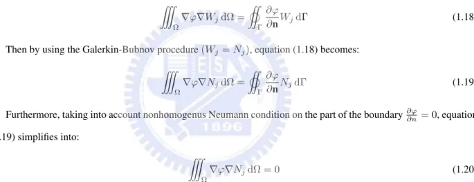
obtained: ˚ Ω ∇ϕ∇WjdΩ = " Γ ∂ϕ ∂nWjdΓ (1.18)

Then by using the Galerkin-Bubnov procedure (Wj= Nj), equation (1.18) becomes:

˚ Ω ∇ϕ∇NjdΩ = " Γ ∂ϕ ∂nNjdΓ (1.19)

Furthermore, taking into account nonhomogenus Neumann condition on the part of the boundary∂ϕ_∂n = 0, equation (1.19) simplifies into:

˚

Ω

∇ϕ∇NjdΩ = 0 (1.20)

Using finite element algorithm, the unknown solution (potential) on the element is expressed by linear combination of shape functions: e ϕe₌ 4 X i=1 αiNi (1.21) `s ds ϕs ϕh (m) (in.) (kV) (kV) Standard condition 0.4 14 15 0

or using matrix notation: e ϕe_{= {N}}T_{{α} = [N} 1 N2 N3 N4]           α1 α2 α3 α4           (1.22)

where vector {α} represents unknown coefficients of the solution, and shape functions are given by:

Ni(x, y, z) = 1

D(Vi+ aix + biy + ciz) for i=1,2,3,4, (x, y, z) ∈ e (1.23)

Combining equations (1.20) to (1.23) results in the global matrix system:

[a]{α} = {Q} (1.24)

where {Q} represents the flux vector. Global matrix [a] is composed from local finite element matrices [a]e

ij.

Potential gradient is defined as:

∇ eϕ =∂ eϕ ∂x − →_e x+∂ eϕ ∂y − →_e y+∂ eϕ ∂z − →_e z (1.25)

and expressed in terms of shape functions is given by:

∇ eϕ =       ∂ eϕ ∂x ∂ eϕ ∂y ∂ eϕ ∂z      =       ∂N1 ∂x ∂N∂x2 ∂N∂x3 ∂N∂x4 ∂N1 ∂y ∂N2 ∂y ∂N3 ∂y ∂N4 ∂y ∂N1 ∂z ∂N∂z2 ∂N∂z3 ∂N∂z4                 α1 α2 α3 α4           . (1.26)

Combining equation (1.20) and (1.26) yields the finite element matrix :

[a]e= ˚ Ωe           ∂N1 ∂x ∂N1 ∂y ∂N1 ∂z ∂N2 ∂x ∂N∂y2 ∂N∂z2 ∂N3 ∂x ∂N∂y3 ∂N∂z3 ∂N4 ∂x ∂N4 ∂y ∂N4 ∂z                 ∂N1 ∂x ∂N∂x2 ∂N∂x3 ∂N∂x4 ∂N1

∂y ∂N∂y2 ∂N∂y3 ∂N∂y4

∂N1 ∂z ∂N∂z2 ∂N∂z3 ∂N∂z4      dΩ. (1.27)

Having computed the scalar potential distribution one may determine the electrostatic field from expression:

− →

Chapter 2

The methods of solving Elliptic PDEs

2.1

Separation of variables to construct solutions of system of Laplace’s

equation.

2.1.1

The domain is a rectangular (dimension = 2) in orthogonal coordinates.

Consider

uxx+ uyy = 0 for 0 < x < π, 0 < y < π. (2.1)

We may apply separation of variables to the equation (2.1) with the form u(x, y) = X(x)Y (y) and divide by u. The process gives

X00 X + Y00 Y = 0, or X00 X = − Y00 Y . (2.2)

The left-hand side of the equation (2.2) depends only upon x and the right-hand side is independent of x. If we take the partial derivative with respect to x,

we find that d dx[ X00 X ] = 0. It follows that X00 X = −λ where λ is a constant.

By the equation (2.2), we find

Y00

Y = λ.

Thus u = X(x)Y (x) is a solution of Laplace’s equation if and only if X(x) and Y(y) satisfy the two ordinary differential equations      X00_{+ λX = 0,} Y00_{− λY = 0.}

The homogeneous problem always has the trivial solution X ≡ 0, but this is no use to us. We are interested in case to find the non-trivial solution of X(x). Since we can see the relationship between λ and X(x) in the previous paper [1], we focus only on the changing of the boundary condition.

Case1

uxx+ uyy = 0 for 0 < x < π, 0 < y < π, (2.3)

u(0, y) = u(π, y) = u(x, π) = 0, (2.4)

u(x, 0) = x2_{(π − x). (2.5)}

If we consider those solutions of the equation which satisfy these conditions, we must have

X00_{+ λX = 0 for 0 < x < π, (2.6)}

X(0) = X(π) = 0. (2.7) and

Y00_{− λY = 0 for 0 < y < π, (2.8)}

Y (π) = 0. (2.9)

Considering the equation (2.6), the general solution is X(x) = a sin√λx + b cos√λx where a, b are determined to

satisfy boundary conditions (2.7). So we have      X(0) = a × 0 + b × 1 = b = 0, X(π) = a sin√λπ = 0. (2.10)

It implies either a = 0 =⇒ X(x) = 0 (trivial solution) or sin√λπ = 0 =⇒√λπ = nπ =⇒ λ = n2_,n=1,2,... We have λ = n2_{= λ} n. Thus Xn(x) = sin √

λnx is the solution of X(x) system (2.6), (2.7) when λ = n2= λn.

In equation (2.8); for each λn, we have linear independent solutions e √

λny_{and e}−

√

λny_{. Thus we get the general} solution of Yn(y) = a e

√

λny _{+ b e}−

√

λny _{where a, b are constants. By boundary condition (2.9), we get Y}

n(π) = a e√λnπ+ b e− √ λnπ = 0. It implies a = −e− √ λnπ 2 and b = e √ λnπ 2 . ⇒ Yn(y) = 1 2(e √ λnπ_e− √ λny_{− e}− √ λnπ_e √ λny_{) = sinh} p_λ n(π − y).

For each λn= n2, Xn(x) = sin nx and Yn(y) = sinh n(π − y). We have constructed the particular solutions

un(x, y) = Xn(x) Yn(y) = sin nx sinh n(π − y) (2.11)

of the system (2.3), (2.4). Any finite linear combinations of un(x, y) is also a solution of the system (2.3), (2.4). We

attempt to represent the solution u as an infinite series in terms of un:

u(x, y) =

∞

X

n=1

cnsin nx sinh n(π − y). (2.12)

We need to determine the coefficients cnso as to satisfy the nonhomogeneous boundary condition (2.5). Thus, setting

y=0 in (2.12), the coefficients

bn = cnsinh nπ,

must satisfy the relation

x2_{(π − x) =} ∞

X

n=1

bnsin nx. (2.13)

The expansion of an arbitrary function in a series of eigenfunctions is called a Fourier series. The particular case where the eigenfunctions are all sines is called a Fourier sine series. If we define

< f (x), g(x) >:= ˆ _π 0 f (x)g(x) dx, then bn= < x 2_{(π − x), sin nx >} < sin nx, sin nx > . (2.14)

Thus we find u(x, y) = −4 ∞ X n=1 [1 + 2(−1)n]n−3sinh n(π − y) sinh nπ sin nx. (2.15)

In order to verify the function u represented by the series (2.15), with bn given by (2.14) is the solution of the

problem (2.3), (2.4) and (2.5), we should check whether the nonhomogeneous boundary condition f (x) = x2_{(π − x)}

is continuous and piecewise smooth on [0, π] and that f (0) = f (π) = 0. Then the Fourier sine series (2.13) of

x2_{(π − x) coverges absolutely and uniformly to the function on [0, π].}

Now, for y ≥ 0,

∞

X

n=1

|cnsin nx sinh n(π − y)| ≤ ∞ X n=1 c e−ny 1 − e−2π (c = 2 π ˆ π 0 |f (x)| dx = π3 6 )

where the series on the right converges. Therefore, the series (2.15) converges absolutely and uniformly to u(x,y) for 0 ≤ x ≤ π and 0 ≤ y ≤ π. Since each term of the series is continuous and satisfies boundary conditions (2.4), (2.5), it follows that u, too (see [8]).

There remains to be verified that the series (2.15) satisfies the Laplace’s equation (2.3). Since the series for ∂u

∂x,∂u∂y,

∂2_u

∂x2 and ∂

2_u

∂y2 are all dominated by a constant times

P

n2_e−ny_{which is converge uniformly for any y > 0, it follows}

that these derivative of u exist and may be obtained by term-by-term differentiation. We see that

uxx+ uyy = ∞

X

n=1

cnsinh n(π − y) sin nx[−n2+ n2] = 0.

The completes the verification that (2.12) with (2.14) is a solution of the problem (2.3), (2.4), (2.5) under the conditions that nonhomogeneous boundary condition is continuous and piecewise smooth on [0, π] and vanishes at the end points.

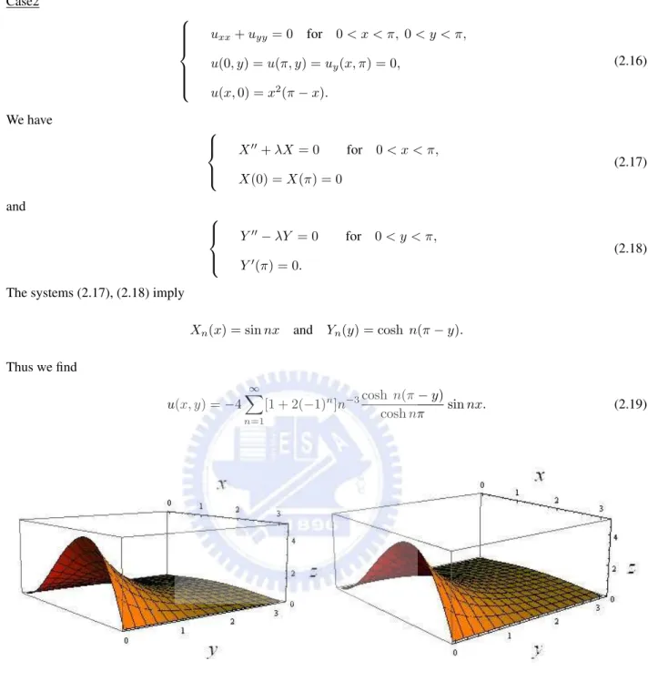
Case2            uxx+ uyy = 0 for 0 < x < π, 0 < y < π, u(0, y) = u(π, y) = uy(x, π) = 0, u(x, 0) = x2_{(π − x).} (2.16) We have      X00_{+ λX = 0 for 0 < x < π,} X(0) = X(π) = 0 (2.17) and      Y00_{− λY = 0 for 0 < y < π,} Y0_{(π) = 0.} (2.18) The systems (2.17), (2.18) imply

Xn(x) = sin nx and Yn(y) = cosh n(π − y).

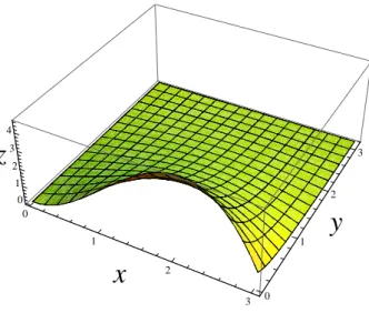
Thus we find u(x, y) = −4 ∞ X n=1 [1 + 2(−1)n_]n−3cosh n(π − y) cosh nπ sin nx. (2.19)

Figure 2.2: The graphic of the case2 where the boundary conditions are u(0, y) = u(π, y) = uy(x, π) = 0 and the

comparison between the graphic and the Figure 2.1.

Case3            uxx+ uyy = 0 for 0 < x < π, 0 < y < π, u(0, y) = ux(π, y) = u(x, π) = 0, u(x, 0) = x2_{(π − x).} (2.20)

We have      X00_{+ λX = 0 for 0 < x < π,} X(0) = X0_{(π) = 0} (2.21) and      Y00_{− λY = 0 for 0 < y < π,} Y (π) = 0. (2.22)

The systems (2.21), (2.22) imply

Xn(x) = sin(n − 1

2)x and Yn(y) = sinh (n − 1 2)(π − y). Thus we find u(x, y) = 8 π ∞ X n=1 [(−24 + π2_{(1 − 2n)}2₎₍₋₁₎n_{+ 4π(1 − 2n)]} (1 − 2n)4 sinh(n − 1 2)(π − y) sinh(n − 1 2)π sin(n − 1 2)x. (2.23)

Figure 2.3: The graphic of the case3 where the boundary conditions are u(0, y) = ux(π, y) = u(x, π) = 0 and the

comparison between the graphic and the Figure 2.1.

Case4            uxx+ uyy = 0 for 0 < x < π, 0 < y < π, ux(0, y) = u(π, y) = u(x, π) = 0, u(x, 0) = x2_{(π − x).} (2.24) We have      X00_{+ λX = 0 for 0 < x < π,} X0_{(0) = X(π) = 0} (2.25)

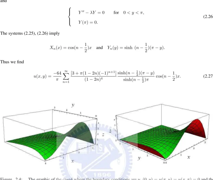
and      Y00_{− λY = 0 for 0 < y < π,} Y (π) = 0. (2.26)

The systems (2.25), (2.26) imply

Xn(x) = cos(n −1

2)x and Yn(y) = sinh (n − 1 2)(π − y). Thus we find u(x, y) = −64 π ∞ X n=1 [3 + π(1 − 2n)(−1)n+1_] (1 − 2n)4 sinh(n − 1₂)(π − y) sinh(n − 1₂)π cos(n − 1 2)x. (2.27)

Figure 2.4: The graphic of the case4 where the boundary conditions are ux(0, y) = u(π, y) = u(x, π) = 0 and the

comparison between the graphic and the Figure 2.1.

Considering Figure 2.1, we see the boundary condition (2.5) decides the graphic in the boundary y = 0 and the figures in other sides (y = π, x = 0, x = π) are determined on the boundary equations (2.4). Moreover, the Maximum Principle tells that the maximum value of u(x,y) always appears on the boundary. Undering the different kind of the boundary conditions, the system (2.19) shows that even though we differentiate u(x,y) respect to y in the boundary condition. The distinct solutions of the case1 and case2 don’t make any difference between Figure 2.1 and Figure 2.2. The Figure 2.3 and 2.4 show that the boundary conditions which are differentiated respect to x will change the shape in that side.

2.1.2

The domain is a disk (dimension = 2) in polar coordinates

We consider a solution u of Laplace’s equation in the unit disk with values given on the boundary. It is natural to introduce the polar coordinates

r =px2_{+ y}2 _{and θ = tan}−1_{(y/x). (2.28)}

A computation shows that Laplace’s equation in these coordinates is

∂2_u ∂r2 + 1 r ∂u ∂r + 1 r2 ∂2_u ∂θ = 0 for r < 1, (2.29) u(1, θ) = f (θ). (2.30) The function f (θ) is a given continuously differentiable function which is periodic of period 2π. The solution

u(r, θ) must also be periodic of period 2π in θ. We may apply separation of variables to (2.29), (2.30) with the form u(r, θ) = R(r)Θ(θ) as detail in [1]. There is another way to show the answer of the system (2.29), (2.30).

If f (θ) is absolutely integrable, we seek a solution of the problem (2.29), (2.30) with the form

u(r, θ) = 1 2a0+ ∞ X n=1 (anrncos nθ + bnrnsin nθ). (2.31)

Therefore anand bnare the Fourier coefficients of f (θ),

an =_π1 ´_π −πf (φ) cos nφ dφ, bn= 1_π ´π −πf (φ) sin nφ dφ. Thus we find u(r, θ) = 1 π ˆ π −π f (φ)[1 2+ ∞ X n=1 rn_{cos n(θ − φ)] dφ. (2.32)}

To evaluate the series,

[r2+ 1−2r cos θ] ∞ X n=1 rncos nθ = ∞ X n=1

{[rn+2_{+ r}n_{] cos nθ − r}n+1_{[cos(n + 1)θ + cos(n − 1)θ]}}

= ∞ X n=1 rn+2_{cos nθ +} ∞ X n=1 rn_{cos nθ −} ∞ X n=2 rn_{cos nθ −} ∞ X n=0 rn+2_{cos nθ} = r cos θ − r2. Then [r2+ 1 − 2r cos θ][1 2 + ∞ X n=1 rncos nθ] =1 2(1 − r 2₎

and 1 2 + ∞ X n=1 rn_{cos nθ =} 1 − r2 2[r2_{+ 1 − 2r cos θ]}. (2.33)

Replacing θ by θ − φ, we find that if´|f (θ)| dθ is finite, the series solution (2.32) can be represented as the integral u(r, θ) = 1 − r 2 2π ˆ _π −π f (φ) 1 + r2_{− 2r cos(θ − φ)}dφ (2.34)

for r < 1. This is called Poisson’s integral formula. If boundary problem is on a circle of radius R, the series can also be written in the form as

u(r, θ) = R2− r2 2π ˆ _π −π f (φ) r2_{+ R}2_{− 2rR cos(θ − φ)}dφ for r < R. (2.35)

This is the general form of Poisson’s integral formula.

These formulas again represent a continuous solution when we define u(R, θ) = f (θ) is continuous and periodic and´f02_{dθ is finite. Furthermore, the series (2.31) or the Poisson integral (2.35) satisfies Laplace’s equation under}

´_π

−π|f | dθ is finite.

Now, we solve the system (2.36), (2.37) by the Green function. Assume the dimension is n (n ≥ 2), and

− → X = (x1, x2, . . . , xn) and−→Y = (y1, y2, . . . , yn). If u(−→X ) satisfies 4u = 0 in B0_{(0, r), (2.36)} u = g on ∂B(0, r), (2.37) then u(−→X ) = r 2₋°°_°−→_X°°_°2 nα(n) ˆ ∂B(0,r) g(−→Y ) ° ° °−→X −−→Y ° ° °n dS(−→Y ) (2.38)

where nα(n) is the surface area of ball with radius r in Rn_{(see [4]).}

Example I: urr+1 rur+ 1 r2uθθ= 0 for r < 1, (2.39) u(1, θ) = sin3θ. (2.40)

Answer :

since r =px2_{+ y}2_{and θ = tan}−1_{(y/x), the system (2.39), (2.40) can be transformed into}

uxx+ uyy = 0 for x2+ y2< 1, (2.41)

u(x, y) = y3 for x2+ y2= 1. (2.42) We can solve the system (2.39), (2.40) by separation of variables. The answer is

u(r, θ) = 1

4(3r sin θ − r3sin 3θ).

(= u(x, y) = 1

4(3y − 3yx2+ y3))

(2.43)

If we solve the system (2.41), (2.42) by the Green function, we get the answer

u(x1, x2) = 1 − (x 2 1+ x22) 2π ˆ ∂B(0,1) y3 2 (x1− y1)2+ (x2− y2)2 dS(−→Y ). (2.44)

Claim : The answers (2.43) and (2.44) are identical

u(x1, x2) = 1 − (x 2 1+ x22) 2π ˆ ∂B(0,1) y3 2 (x1− y1)2+ (x2− y2)2dS( − → Y ) (y1= cos θ, y2= sin θ, dS(−→Y ) = dθ.) = 1 − (x 2 1+ x22) 2π ˆ 2π 0 sin3_θ (x1− cos θ)2+ (x2− sin θ)2dθ

(By Residue Theorey, let cos θ = 1

2(z +z1) and sin θ = 2i1(z −1z). Thus we find dθ = dziz.)

= 1 − (x 2 1+ x22) 2π ˆ c 1 8z(z − 1 z)3 [x1−12(z +z1)]2+ [x2−2i1(z −1z)]2 dz = 1 − (x 2 1+ x22) 16π(−x1+ ix2) ˆ c (z2_{− 1)}3 z3_{(z −} 1 x1−ix2)(z − (x1+ ix2)) dz.

Let α1=_x1−ix1 ₂, and α2= x1+ ix2. We find

f (z) = (z 2_{− 1)}3 z3_{(z −} 1 x1−ix2)(z − (x1+ ix2)) = (z2− 1)3 z3_{(z − α} 1)(z − α2) .

only consider the Res(f;α2) and Res(f;0). It implies I = [1 − (x 2 1+ x22)](−2α1πi) 16π [Res(f ; α2) + Res(f ; 0)] (2.45) where Res(f ; α2) = lim z→α2 (z − α2)f (z) = (α 2 2− 1)3 α3 2(α2− α1), Res(f ; 0) = lim z→0 d2 dz2[z 3_{f (z)] =} 1 α2− α1( 3 α1 − 3 α2 − 1 α3 1 + 1 α3 2 ). Thus we find I = 1 4(x 3 2+ 3x2− 3x21x2) = u(x1, x2). Example II :            ∂2_u ∂r2 +1_r∂u_∂r+_r12∂ 2_u ∂θ = 0 for r < 1, 0 < θ < π 2, u(r, 0) = uθ(r,1₂π) = 0, u(1, θ) = θ. (2.46) Answer :

Using separation of variables, we get

u(r, θ) = 4 π ∞ X n=1 (−1)n+1 (2n − 1)2sin(2n − 1)θ r 2n−1_{. (2.47)}

If we transform the system (2.47) from Polar coordinate into Cartesian coordinate, we get                    uxx+ uyy = 0 for x2+ y2< 1, 0 < tan−1(yx) < π2, u(x, y) = 0 for y = 0,

−ux(x, y)y2= 0 for x = 0,

u(x, y) = tan−1₍y

x) for x2+ y2= 1.

(2.48)

The solution of the problem (2.47) will also be the solution of the problem (2.48)

u(r, θ) = u(x, y) = ∞ X n=1 4(−1)n+1 π(2n − 1)2sin[(2n − 1) tan −1₍y x)](x 2_{+ y}2₎2n−1 2 . (2.49)

2.1.3

The domain is a cube (dimension = 3) in orthogonal coordinates

Consider

∇2u = uxx+ uyy+ uzz= 0 for 0 < x < π, 0 < y < π, 0 < z < π, (2.50)

u = 0 for x = 0 and π, y = 0 and π, z = π, (2.51)

u(x, y, 0) = g(x, y). (2.52)

We apply the method of separation of variables to a product function V (x, y, z) = X(x)Y (y)Z(z) which solves the system (2.50), (2.51) and (2.52). We have

X00 X +Y 00 Y = −Z 00 Z = C1and X00 X = C1−Y 00 Y = C2 (2.53)

where C1and C2 are constants. The homogeneous boundary conditions (2.51) give

X(0) = X(π) = 0, Y (0) = Y (π) = 0, Z(π) = 0.

(2.54)

By the systems (2.53) and the boundary conditions (2.54), we get three ODE systems      X00_{− C} 2X = 0, X(0) = X(π) = 0. (2.55)      Y00_{− (C} 1− C2)Y = 0, Y (0) = Y (π) = 0. (2.56)      Z00_{+ C} 1Z = 0, Z(π) = 0. (2.57)

By the systems (2.55), (2.56) , we get Xn(x) = sin nx and Ym(y) = sin my. It implies C2 = −n2and C1− C2 =

−m2_{, then C}

1= −m2− n2. So that the system (2.57) shows Z(z) = sinh

√ m2_{+ n}2_{(π − z). We seek a solution of} the form u(x, y, z) = ∞ X n=1 ∞ X m=1 αnmsinh p

By the boundary condition (2.52), we obtain g(x, y) = ∞ X n=1 ∞ X m=1 αnmsinh p

m2_{+ n}2_{π sin nx sin my.}

Therefore, αnmsinh p m2_{+ n}2_{π = δ} nm= 4 π2 ˆ _π 0 ˆ _π 0 g(x, y) sin nx sin my dx dy and u(x, y, z) = ∞ X n=1 ∞ X m=1 δnmsinh √ m2_{+ n}2_{(π − z)}

sinh√m2_{+ n}2_π sin nx sin my. (2.59)

Since we must verify that the series (2.59) gives a solution to the system (2.50), (2.51) and (2.52), we should check whether´₀π´₀π|g| dx dy is finite. (the δnm are uniformly bounded). Then the series (2.59) and all its derivatives

converge absolutely and uniformly for z0 ≤ z ≤ π, 0 ≤ x ≤ π, 0 ≤ y ≤ π for any constant z0 > 0. It follows that

u(x, y, z) is infinitely differentiable for z > 0 and satisfies Laplace’s equation.

In order to sure that u satisfies the boundary condition at z=0, we should check whether g(x,y) is continuous and continuously differentiable and the squares of its second partial derivatives have finite integrals, then the double Fourier series converges absolutely and uniformly to g(x,y) as a double series (see [2]).

Example: ∇2u − u = 0 for 0 < x < π, 0 < y < π 2, 0 < z < 1, (2.60) u = 0 for x = 0, y = 0, z = 1, (2.61) ux= 0 for x = π, (2.62) uy = 0 for y = π 2, (2.63) uz(x, y, 0) = 2x − π. (2.64) Answer :

and (2.64), we have X00_{Y Z + XY}00_{Z + XY Z}00_{− XY Z = 0.} =⇒X 00 X + Y00 Y + Z00 Z − 1 = 0 =⇒X 00 X + Y00 Y = − Z00 Z + 1 = C1 =⇒X00 X = C1− Y00 Y = C2

where C1and C2are constants. The homogenous boundary conditions (2.61), (2.62) and (2.63) give

X(0) = X0_{(π) = 0,}

Y (0) = Y0₍π

2) = 0,

Z(1) = 0.

Thus, we get three ODE systems _     X00_{− C} 2X = 0, X(0) = X0_{(π) = 0.} (2.65)      Y00_{− (C} 1− C2)Y = 0, Y (0) = Y0₍π 2) = 0. (2.66)      Z00_{+ (C} 1− 1)Z = 0, Z(1) = 0. (2.67)

By the system (2.65), we have C2= (n −1₂)2with correspond eigenfunction

Xn(x) = sin(n −1

2)x and the system (2.66) implies

Ym(y) = sin(2m − 1)y,

hence C1− C2= −(2m − 1)2and C1− 1 = −[(n −1₂)2+ (2m − 1)2− 1].

By the system (2.67), we get

Z(z) = sinh

r (n −1

2)2+ (2m − 1)2+ 1(1 − z). We seek the solution of form

u(x, y, z) = ∞ X n=1 ∞ X m=1 αnmsin(n −1

2)x sin(2m − 1)y sinh r

(n −1

By the boundary condition (2.64), we make − q (n −1 2)2+ (2m − 1)2+ 1 cosh( q (n −1 2)2+ (2m − 1)2+ 1)αnm= δnm = ˆ π 2 0 ˆ π 0 (2x − π) sin(n −1 2)x sin(2m − 1)y dx dy ˆ π 2 0 ˆ _π 0 sin2_{(n −}1 2)x sin 2_{(2m − 1)y dx dy} = −8 π ( 1 n−1 2 + 2(−1)n π(n−1 2)2) 2m − 1 . =⇒ αnm= 8( 1 n−1 2 + 2(−1)n π(n−1 2)2) π(2m − 1) q (n −1 2)2+ (2m − 1)2+ 1 cosh( q (n −1 2)2+ (2m − 1)2+ 1) and u(x, y, z) = 8 π ∞ X n=1 ∞ X m=0 ( 1 n −1 2 + 2(−1)n π(n −1 2)2 ) sin(n − 1

2)x sin(2m − 1)y sinh

q (n −1₂)2_{+ (2m − 1)}2_{+ 1(z − 1)} (2m − 1) q (n −1 2)2+ (2m − 1)2+ 1 cosh( q (n −1 2)2+ (2m − 1)2+ 1) (2.69)

Figure 2.5: The projection of the solution (2.69) on the z = 0, 1

4, 12 (brown, red, green) .

Because we doubt if the graphics of u(x, y, 0), u(x, y,1

4) and u(x, y,12) would intersect at the same line in the

region [1.4, 1.6] × [0, 2] on the xy-plane, we use the numerical method to show the values in Appendix B.1, and the answer is no.

2.1.4

The domain is a cylinder (dimension = 3) in cylindrical coordinates

If we introduce cylindrical coordinates r, θ, z such that

x = r cos θ, y = r sin θ, z = z.

Laplace’s equation in cylindrical coordinates becomes

∂2_u ∂r2 + 1 r ∂u ∂r+ 1 r2 ∂2_u ∂θ2 + ∂2_u ∂z2 = 0 for 0 < r < R1, 0 < z < π, (2.70) u(r, θ, 0) = u(r, θ, π) = 0, (2.71) u(R1, θ, z) = g(θ, z). (2.72)

Consider the product function V (r, θ, z) = R(r)Θ(θ)Z(z) such that V (r, θ, z) solves the system (2.70), (2.71) and (2.72). Then R00₊1 rR0 R + 1 r2 Θ00 Θ = − Z00 Z = C1 (2.73) andr 2_R00_{+ rR}0 R − r 2_C 1= −Θ 00 Θ = C2 (2.74)

where C1and C2 are constants.

By the boundary conditions (2.71) and the equation (2.73), we have      Z00_{+ C} 1Z = 0, Z(0) = Z(π) = 0. It implies that Zn(z) = sin nz with C1= n2, n = 1, 2 . . . .

Considering that Θ is periodic of period 2π, then            Θ00_{+ C} 2Θ = 0, Θ(0) = Θ(2π), Θ0_{(0) = Θ}0_(2π).

Then C2= m2, m = 0, 1, 2, . . ., and the corresponding eigenfunctions are

Θ0= 1, Θm= sin mθ, cos mθ. (m = 1, 2, . . . are double eigenvalues)

Finally, we obtain the differential equation

Rmn00 + 1 rR 0 mn− ( m2 r2 + n 2_)R mn= 0, (2.75) Rmn(R1) = 1. (2.76)

This equation is singular at r=0. In place of a boundary condition we impose the condition that R remain finite at r=0. (Frobenius method) We seek a solution of the form

Rmn(r) = γ ∞

X

k=0

ckrα+k c06= 0 and α, γ are constants.

By the equation (2.75), we have (α + k)2 ∞ X k=0 ckrα+k−1− m2 ∞ X k=0 ckrα+k−1− n2 ∞ X k=0 ckrα+k+1 = α2_c 0rα−1+ (α + 1)2c1rα− m2c0rα−1− m2c1rα+ ∞ X k=2 ([(α + k)2_{− m}2_]c k− n2ck−2)rα+k−1 = {(α2_{− m}2_)c 0+ [(α + 1)2− m2]c1r}rα−1+ ∞ X k=2 ([(α + k)2_{− m}2_]c k− n2ck−2)rα+k−1= 0.

The power series is identically zero only if all its coefficients vanish. It implies that

α = ±m, c1= 0 and cι = n 2_c ι−2 (α + ι)2_{− m}2. Hence c1= c3= c5= . . . = 0 and c2= n 2_c 0 [(α + 2)2_{− m}2_] c4= n2_c 2 (α + 4)2_{− m}2 = n4_c 0 [(α + 4)2_{− m}2_{][(α + 2)}2_{− m}2_] .. . c2ι = n 2ι_c 0 [(α + 2ι)2_{− m}2_{][(α + 2(ι − 1))}2_{− m}2_{] . . . [(α + 2)}2_{− m}2_]. Thus we find ∞ X k=0 ckrα+k = c0rα+ ∞ X k=1 ckrα+k = c0rα+ ∞ X ι=1 c2ιrα+2ι = c0rα[1 + ∞ X ι=1 (rn)2ι [(α + 2ι)2_{− m}2_{][(α + 2(ι − 1))}2_{− m}2_{] . . . [(α + 2)}2_{− m}2_]].

If we choose α = m and define c0= n

m 2m_·m!, then Rmn(r) = γ ∞ X ι=0 n2ι+m₍1 2r)m+2ι ι!(ι + m)! = γJm(nr) (2.77)

where Jmis the Bessel function that converges for all r (see [2]).

By the boundary condition (2.76),

γ = 1

Jm(nR1) =⇒ Rmn(r) =

Jm(nr)

We seek the solution u in the form u(r, θ, z) =1 2 ∞ X n=1 cn0 J0(nr) J0(nR1) sin nz + ∞ X n=1 ∞ X m=1 Jm(nr) Jm(nR1)

sin nz(cnmcos mθ + dnmsin mθ) (2.78)

where cnm= 2 π2 ˆ _π 0 ˆ _2π 0 g(θ, z) sin nz cos mθ dθ dz, dnm= 2 π2 ˆ π 0 ˆ 2π 0 g(θ, z) sin nz sin mθ dθ dz.

Similarly, we should verify the series (2.78) satisfies the problem (2.70), (2.71), (2.72). We must check if |g(θ, z)| and its second partial derivatives have finite integrals.

Example: ∇2_{u = 0 for 0 < r < 1, 0 < z < π, (2.79)} u(r, θ, 0) = 0, (2.80) uz(r, θ, π) = 0, (2.81) u(1, θ, z) = z cos3_{θ. (2.82)} Answer :

By separation of variables, we obtain three ODE systems      Z00_{+ C} 1Z = 0, Z0_{(π) = Z(0) = 0.} (2.83)      Θ00_{+ C} 2Θ = 0, Θ(0) = Θ(2π) and Θ0_{(0) = Θ}0_(2π). (2.84)      R00 mn+1rR0mn− ((n − 12)2+ (mr)2)Rmn= 0,

Rmn remain finite at r=0 and Rmn(1) = 1.

(2.85)

The systems (2.83) , (2.84) imply

Zn(z) = sin(n − 1

2) with C1= (n − 1 2)

and C2= m2, m = 0, 1, 2, . . . with the corresponding eigenfunctions

Θ0= 1, Θm= sin mθ, cos mθ. (m = 1, 2, . . . are double eigenvalues)

By the system (2.85), we let

Rmn(r) = ` ∞

X

k=0

ckrk+αwith c06= 0, ` and α are constants.

We have {(α2− m2)c0+ [(α + 1)2− m2]c1r}rα−1+ ∞ X k=2 ([(α + k)2− m2]ck− (n −1 2) 2_c k−2)rα+k−1= 0.

The power series is identically zero only if all its coefficients vanish, it implies

α = ±m, c1= 0 and cι = (n −1 2)2cι−2 (α + ι)2_{− m}2. =⇒ Rmn(r) = γ ∞ X ι=0 (n −1 2)2ι+m(12r)m+2ι ι!(ι + m)! = γIm((n − 1 2)r). Since Rmn(1) = 1, it implies Rmn(r) = Jm((n− 1 2)r)

Jm(n−12) . We get the solution u in the form

u(r, θ, z) = 1 2 ∞ X n=1 cn0 J0((n −1₂)r) J0(n −1₂) sin(n − 1 2)z + ∞ X n=1 ∞ X m=1 Jm((n −1₂)r) Jm(n −1₂) sin(n − 1 2)z(cnmcos mθ + dnmsin mθ) where dnm= ´π 0 ´2π

0 z cos3θ sin(n −12)z sin mθ dθ dz

´_π 0 ´_2π 0 (sin(n − 1 2)z)2(sin mθ)2dθ dz = 0, (∵ ˆ 2π 0 z cos3_{θ sin mθ dθ = 0 ∀m)} cnm= ´_π 0 ´_2π

0 z cos3θ sin(n −12)z cos mθ dθ dz

´π 0 ´2π 0 (sin(n −12)z)2(cos mθ)2dθ dz =                (−1)n+1 (n −1 2)2 3π 4 for m = 1, (−1)n+1 (n −1 2)2 π 4 for m = 3, 0 otherwise. Then solution u is u(r, θ, z) = 3 2π ∞ X n=1 sin(n −1 2)z cos θ J1((n −1₂)r) J1(n −1₂) + 1 2π ∞ X n=1 sin(n −1 2)z cos 3θ J3((n −1₂)r) J3(n −1₂) .

2.1.5

The domain is a sphere (dimension = 3) in spherical coordinates

If we introduce spherical coordinates r, θ, φ such that

x = r sin θ cos φ, y = r sin θ sin φ, z = r cos θ,

then Laplace’s equation becomes

∂2_u ∂r2 + 2 r ∂u ∂r + 1 r2_{sin θ} ∂ ∂θ(sin θ ∂u ∂θ) + 1 r2_sin2_θ ∂2_u ∂φ2 = 0 for r < R, (2.86) u(R, θ, φ) = f (θ, φ). (2.87)

Applying separation of variables, we find that the equation (2.86) has solutions of the form R(r)Θ(θ)Φ(φ). It yields that R00₊2 rR0 R + (sinθΘ0₎0 Θr2_{sin θ} + Φ00 Φr2_sin2_θ = 0.

Multiplying by r2_sin2_{θ and transposing the last term, we see}

(r2_{sin θ)}R00+2rR0

R +

(sinθΘ0₎0

Θ = −

Φ00

Φ = c where c is a constant and c ≥ 0.(if c < 0, we will get Φ ≡ 0) Since Φ must be periodic of period 2π, we have Φ = cos mφ or sin mφ where m=0,1,. . .

Then R00₊2 rR0 R + (sinθΘ0₎0 Θr2_{sin θ} − m2 r2_sin2_θ = 0. We get r2_R00_{+ 2rR}0 R = m2 sin2θ − (sinθΘ0₎0

Θ sin θ = λ where λ is a constant. We get two equations

r2(R00+2

rR

0_{) − λR = 0. (2.88)}

(sin θΘ0₎0₋ m2

sin θΘ + λ sin θΘ = 0. (2.89)

The equation (2.89) for Θ(θ) is singular at its two endpoints θ = 0 and θ = π. We impose the condition that Θ and Θ0_{remain bounded at both ends. This gives an eigenvalue problem with two singular endpoints. Let t = cos θ and}

Θ(θ) = P (cos θ). Then equation (2.89) becomes

d dt[(1 − t 2₎dP dt] − m2 1 − t2P + λP = 0 for − 1 < t < 1. (2.90)

If m=0 and λ = 0 in the equation (2.90) , we find the solution P ≡ 1 which is continuously differentiable for

−1 ≤ t ≤ 1. But the eigenfunction P=constant isn’t included in our discussion. Since the eigenvalue λ = ´₁ −1[(1−t2)P02+1−t2m2 P 2_{] dt} ´₁ −1P2dt

≥ 0, we first consider the case m=0 and λ 6= 0. We have d

dt[(1 − t

2₎dP

dt] + λP = 0. (2.91)

We seek a solution in the neighborhood of t=1 as a power series in (t-1)

P (t) = (t − 1)α ∞

X

k=0

ck(t − 1)k c06= 0. (2.92)

By the equation (2.91), we have

−c02α2(t − 1)α−1− ∞

X

k=0

{2(k + α + 1)2ck+1+ [−λ + (k + α + 1)(k + α)]ck}(t − 1)k+α= 0.

The power series is identically zero only if its coefficient vanish, we obtain

α = 0 and ck+1= −[k(k + 1) − λ] 2(k + 1)2 ck. Thus ck= [k(k − 1) − λ][(k − 1)(k − 2) − λ] · · · [2 − λ][−λ](−1) k 2k_(k!)2 c0.

By ratio test we find that the series (2.92) converges for |t − 1| < 2 and in general approach ±∞ as t → −1 except the series terminates. That means the function is bounded for −1 ≤ t ≤ 1 if and only if

λ = n(n + 1), n = 0, 1 . . .

Setting c0= 1 and we obtain the eigenfunction Pn(t) corresponding to the eigenvalue λn= n(n + 1) is

Pn(t) = n X k=0 (n + k)! (n − k)!(k!)2₂k(t − 1) k_.

Pn(t) is a polynomial of degree n in t. It is called a Legendre polynomial. Since Pk(t) of degree k can be

expressed as a linear combination of Pn(t) with n = 0, 1, . . . k and Pnare orthogonal, it implies

ˆ ₁

−1

tkPn(t) dt = 0 for k = 0, 1, . . . , n − 1.

So we can verify the identity

Pn(t) = 1

2n_n!

dn

dtn(t

2_{− 1)}n_,

which is called the Rodrigues formula.

If m 6= 0 and n ≥ m, the eigenfunction corresponds to the eigenvalue λ = n(n + 1) is

Pm n (t) ≡ (1 − t2)m/2 dm dtm[Pn(t)] = 1 2n_n!(1 − t 2₎m/2dm+n dtm+n(t 2_{− 1)}n

and called the associated Legendre function.

The method of separation of variables thus gives the harmonic functions

rn_Pm

n (cos θ) cos mφ, rnPnm(cos θ) sin mφ (2.93)

which are regular in the whole (r, θ, φ) space and we call these polynomials spherical harmonics (see [2]). To solve the boundary equation (2.87), we expand f (θ, φ) in a double Fourier series

f (θ, φ) ∼ ∞ X n=0 [1 2an0Pn(cos θ) + n X m=1

(anmcos mφ + bnmsin mφ)Pnm(cos θ)]

where anm=(2n + 1)(n − m)! 2π(n + m)! ˆ 2π 0 ˆ π 0 f (θ, φ)Pm

n (cos θ) cos mφ sin θ dθ dφ,

bnm= (2n + 1)(n − m)! 2π(n + m)! ˆ _2π 0 ˆ _π 0

f (θ, φ)Pnm(cos θ) sin mφ sin θ dθ dφ.

The formal solution of the problem (2.86) and (2.87) is then

u(r, θ, φ) = ∞ X n=0 (r R) n_[1 2an0Pn(cos θ) + n X m=1

(anmcos mφ + bnmsin mφ)Pnm(cos θ)]. (2.94)

Example: _     ∇u = 0 for r < 1, u = x3 _{for r = 1.} (2.95) Answer :

Translate x into spherical coordinates (x = r sin θ cos φ)

=⇒ anm =(2n+1)(n−m)!_2π(n+m)!

´_2π

0

´_π

0 sin3θ cos3φPnm(cos θ) cos mφ sin θ dθ dφ

=(2n+1)(n−m)!_2π(n+m)! ´₀2πcos3_{φ cos mφ dφ} ´π 0 sin 3_θPm n (cos θ) sin θ dθ. Since ˆ _2π 0 cos3φ cos mφ dφ = ˆ _2π 0 (1 4cos 3φ + 3 4cos φ) cos mφ dφ = 1 8{ ˆ _2π 0 [cos(3 + m)φ + cos(3 − m)φ] dφ + 3 ˆ _2π 0 [cos(1 + m)φ + cos(1 − m)φ] dφ} =            π 4 for m=3, 3π 4 for m=1, 0 otherwise.

For m=1,

ˆ π 0

sin3_θP1

n(cos θ) sin θ dθ (cos θ = t)

= ˆ 1 −1 (1 − t2₎3 2P1 n(t) dt = ˆ ₁ −1 (1 − t2₎2dPn(t) dt dt = 4[ ˆ ₁ −1 tPn(t) dt) − ˆ ₁ −1 t3Pn(t) dt] =            16 15 for n=1 ⇒ a11= 35, −16 35 for n=3 ⇒ a31= −101, 0 otherwise. For m=3, ˆ π 0 sin3_θP3 n(cos θ) sin θ dθ =      96 7 for n=3 ⇒ a33= 601, 0 otherwise. =⇒ u(r, θ, φ) = 3 5cos φP 1 1(cos θ) − 1 10cos φP 1 3(cos θ) + 1 60cos 3φP 3 3(cos θ).

2.2

Finite Fourier transform to construct the solution of system of Laplace’s

equation

Consider the non-homogeneous problem

uxx+ uyy= F (x, y) for 0 < x < π, 0 < y < 1, (2.96)

u(x, 1) = u(0, y) = u(π, y) = 0, (2.97)

u(x, 0) = 0. (2.98)

To solve the non-homogeneous problem (2.96), (2.97) and (2.98), we expand the solution in a Fourier sine series for each fixed y.

u(x, y) ∼

∞

X

n=1

bn(y) sin nx.

The set of sine coefficients

bn(y) = 2

π

ˆ _π

0

u(x, y) sin nx dx

which is a function of the integer n and of y, determines u(x,y) uniquely. It is called the fininte sine transform of u(x,y).

If∂2_u

∂x2 is continuous, its finite sine transform is given by

2 π ˆ π 0 ∂2_u ∂x2sin nx dx = 2 π ½· ∂u ∂xsin nx ¸π 0 − n ˆ π 0 ∂u ∂xcos nx dx ¾ = −n2_b n(y). If∂2_u

∂y2 is continuous, we can interchange integration and differentiation to show that

2 π ˆ π 0 ∂2_u ∂y2 sin nx dx = ∂2 ∂y2 · 2 π ˆ π 0 u sin nx dx ¸ = b00_n(y). Taking the finite sine transform of both sides of the equation (2.96) leads to the equation

b00n(y) − n2bn(y) = Bn(y) (2.99)

where Bn(y) = 2 π ˆ π 0 F (x, y) sin nx dx.

The boundary condition (2.98) means that

Taking sine transforms, we have reduced the problem for a partial differential equation to the problem (2.100) for an ordinary differential equation.

     b00

n(y) − n2bn(y) = Bn(y),

bn(0) = bn(1) = 0.

(2.100)

We can use Green’s function to solve the problem (2.100) and the solution has Fourier sine series form. By Schwarz’s inequality and Parseval’s equation, we know that the seriesPbn(y) sin nx converges uniformly for 0 ≤

x ≤ π, 0 ≤ y ≤ 1, then u(x, y) = ∞ X n=1 bn(y) sin nx. Example: Solve     

uxx+ uyy = y(1 − y) sin3x for 0 < x < π, 0 < y < 1,

u(x, 0) = u(x, 1) = u(0, y) = u(π, y) = 0.

(2.101)

Answer :

We expand the solution in a Fourier sine series for each fixed y and we find

u(x, y) =

∞

X

n=1

bn(y) sin nx where bn(y) = 2

π ˆ _π 0 u(x, y) sin nx dx. We have 2 π ˆ _π 0

uxxsin nx dx = −n2bn(y) and

2

π

ˆ _π

0

uyysin nx dx = b00n(y).

Taking the finite sine transform of both sides of (2.101) leads to the second order differential equation                            b00 n(y) − n2bn(y) = _π2 ´_π

0[y(1 − y) sin3x] sin nx dx = f (y) , for 0 < y < 1

=            3 4y(1 − y) for n = 1, −1 4 y(1 − y) for n = 3, 0 otherwise, bn(0) = bn(1) = 0. (2.102)

Now, we use Green’s function to solve the system (2.102) and we have      p(y) = 1 q(y) = −n2 and      α = 0 β = 1

Let v1(y) = enyand v2(y) = e−nywhich satisfy the equation v00− n2v = 0. We have

k = p(y) [v01(y)v2(y) − v02(y)v1(y)] = 2n

and D = v1(α)v2(β) − v1(β)v2(α) = e−n− en. When ξ ≤ x, we have G(x, ξ) = 1 kD[v1(ξ)v2(α) − v1(α)v2(ξ)][v1(x)v2(β) − v1(β)v2(x)] = 1 2n(en_{− e}−n₎[e nξ_{− e}−nξ_][en(1−x)_{− e}−n(1−x)_]. When ξ ≥ x, we have G(x, ξ) = 1 kD[v1(x)v2(α) − v1(α)v2(x)][v1(ξ)v2(β) − v1(β)v2(ξ)] = 1 2n(en_{− e}−n₎[e nx_{− e}−nx_][en(1−ξ)_{− e}−n(1−ξ)_]. So bn(x) = ˆ 1 0 G(x, ξ)f (ξ) dξ = ˆ x 0 G(x, ξ)f (ξ) dξ + ˆ 1 x G(x, ξ)f (ξ) dξ = −1 2n(en_{− e}−n₎{[e n(1−x)_{− e}−n(1−x)_] ˆ _x 0 (enξ_{− e}−nξ_{)f (ξ) dξ} + (enx− e−nx) ˆ 1 x [en(1−ξ)− e−n(1−ξ)]f (ξ) dξ} =          3 4[−x(1 − x) + 2(1 − cosh(x −1 2) cosh1 2 )] for n=1, −1 4[ −1 9 x(1 − x) + 2 81(1 − cosh 3(x −1 2) cosh3 2 )] for n=3. Therefore, the solution is

u(x, y) = 3 4[−y(1 − y) + 2(1 − cosh(y −1 2) cosh1 2 )] sin x −1 4[ −1 9 x(1 − x) + 2 81(1 − cosh 3(y −1 2) cosh3 2 )] sin 3x.

2.3

The Fourier transform to construct the solution of Laplace’s equation

Fourier transform provides a way of expanding functions on the whole real line R=(−∞, ∞) as (continuous) superpo-sitions of the basic oscillatory functions eiwx _{(w ∈ R) in much the same way that Fourier series are used to expand}

functions on a finite interval.

To understand this relationship, consider a function f on R. For any ` > 0 we can expand f on the interval [−`, `] in a Fourier series, and we wish to see what happens to this expansion as we let ` → ∞

For x ∈ [−`, `] f (x) = 1 2` ∞ X n=−∞ cn,`e −iπnx ` where c<sub>n,`</sub>= ˆ <sub>`</sub> −`

f (y)eiπny` dy. (2.103) Let ∆w =π

` and wn = n∆w = nπ` ; then these formulas become

f (x) = 1 2π ∞ X n=−∞ cn,`e−iwnx∆w where cn,`= ˆ ` −` f (y)eiwny_dy.

Suppose that f(x) vanishes rapidly as x → ±∞; then cn,`will not change much if we extend the region of integration

from [−`, `] to (−∞, ∞):

cn,`≈

ˆ ∞ −∞

f (y)eiwny_{dy. (2.104)} The integral function (2.104) only of wn, which we call bf (w), and we now have

f (x) ≈ 1 2π ∞ X n=−∞ b f (w)e−iwx_{∆w (|x| < `). (2.105)}

This looks very much like a Riemann sum. If we now let ` → ∞, so that ∆w → 0. The ≈ should become = and the sum should turn into an integral, thus:

f (x) = 1

2π ˆ ∞

−∞

b

f (w)e−iwx_{dw where bf (w) =}

ˆ ∞ −∞

f (x)eiwx_{dx. (2.106)}

The function bf is called the Fourier transform of f. It is sometimes denoted by F[f ]. And (2.106) is the Fourier

inversion theorem. The integral certainly converges if´_−∞∞ |f (x)| dx does (see [3]).

For function of two variables, say u(x,y), we define F[u](w, y) ≡

ˆ _∞

−∞

Example:                    uxx+ uyy = 0 for − ∞ < x < ∞, 0 < y < 1, u(x, 0) = e−2|x|_{= f (x),} u(x, 1) = 0, u(x, y) → 0 uniformly in y, as x → ±∞. Answer :

F[uxx+ uyy] = F[uxx] + F[uyy]

where F[uyy] = ˆ _∞ −∞ eiwxuyydx = ∂ ∂y2 ˆ _∞ −∞ eiwxu dx = buyy, (∵ u → 0 uniformly in y as x → ±∞ ∴ ux→ 0 uniformly in y as x → ±∞) F[uxx] = ˆ ∞ −∞ eiwx_u xxdx = eiwxux|∞−∞− (iw) ˆ ∞ −∞ eiwx_u xdx = (−iw)[eiwx_{u |}∞ −∞− (iw) ˆ _∞ −∞ eiwx_{u dx] = −w}2_u,b ⇒ F[uxx+ uyy] = −w2bu + buyy = 0, b u(w, 0) = ˆ ∞ −∞ eiwx_{u(x, 0) dx =} ˆ ∞ 0 eiwx_{u(x, 0) dx =} ˆ 0 −∞ eiwx_{u(x, 0) dx.} = lim t→∞[ eiw−2 iw − 2 | t 0] + lim_m→−∞[ eiw−2 iw − 2 | 0 m] = −1 iw − 2+ 1 iw + 2 = 4 w2_{+ 4}. Thus we find − w2_{u + bb u} yy= 0, (2.108) b u(w, 0) = 4 w2_{+ 4} = bf (w), (2.109) b u(w, 1) = 0. (2.110) By the equation (2.108), if bu(x, y) = A(x)ewy_{+ B(x)e}−wy_,

then bu(w, 0) = A(w) + B(w) = 4

w2₊₄ and bu(w, 1) = A(w)ew+ B(w)e−w= 0.

We get A(w) = −2e

−w

sinh w(w2_{+ 4)} and B(w) =

2ew

⇒ bu(x, y) = 4 sinh(x − wy)

sinh x(x2_{+ 4)}.

By inverse fourier theorem,

u(x, y) = 1 2πL→∞lim ˆ L −L e−iwx_{bu(w, y) dw =} 2 π ˆ ∞ −∞ e−iwx sinh w(1 − y) sinh w(w2_{+ 4)}dw.

There is another solution for the special case where u(x,0)=f(x). If f(x) is either the even function or odd function, we can use cosine or sine transform. They are defined respectively as

Fs[f ] ≡ ˆ ∞ 0 f (x) sin wx dx and Fc[f ] ≡ ˆ ∞ 0 f (x) cos wx dx.

Since eiwx_{= cos wx + i sin wx,}

b

f (w) = 2iFs[f ] if f(x) is an odd function at (−∞, ∞),

b f (w) = 2Fc[f ] if f(x) is an even function at (−∞, ∞). ∵ f (x) = e−2|x|_{is an even function ∴ bf (w) = 2F} c[f ]. Fc[uxx] = ˆ _∞ 0

uxxcos wx dx = −w2Fc[u] = −w2U (w, y),

Fc[uyy] = Uyy(w, y), U (w, 0) = ˆ _∞ 0 u(x, 0) cos wx dx = 2 w2_{+ 4}. Thus we find − w2_{U (w, y) + U} yy(w, y) = 0, (2.111) U (w, o) = 2 w2_{+ 4}, (2.112) U (w, 1) = 0. (2.113) To compute the system (2.111), (2.112) and (2.113) with similar way, we have U (w, y) =_(w2 sinh w(1−y)2_{+4) sin hw}.

Thus u(x, y) = 2 π ˆ _∞ 0 U (w, y) cos wx dw = 2 π ˆ ∞ −∞

(cos wx − i sin wx) sinh w(1 − y) (w2_{+ 4) sin hw}dw = 2 π ˆ ∞ −∞ e−iwx sinh w(1 − y) (w2_{+ 4) sin hw}dw.