Novel sampling clock offset estimation for DVB-T OFDM

Novel Sampling Clock Offset Estimation for DVB-T OFDM

Hou-Shin Chen Yumin Lee

Graduate Institute of Communication Eng. and

Department of Electrical Eng.,

National Taiwan University, Taipei 10617, Taiwan

Abstract – Sampling clock offset estimation and compensation

are important problems in an OFDM system. Sampling clock offset can cause a severe drift in symbol-timing, thus causing inter-carrier and inter-OFDM-symbol interference. In this paper, we propose a novel sampling clock offset estimator for OFDM systems that use scattered pilots. The proposed algorithm makes use of the received pilot phases and the least-squares algorithms. Simulation results show that when applied to the DFB-T standard, the performance of the proposed estimator is very accurate and robust against multipath fading and Doppler Spread.

I. INTRODUCTION

Terrestrial Digital Video Broadcasting (DVB-T) is a next-generation standard for wireless broadcast of MPEG-2 video [1]. In order to provide the high data rate required for video transmission, concatenated-coded orthogonal frequency division multiplexing (OFDM) has been adopted into DVB-T. In an OFDM system synchronization includes symbol timing estimation, carrier frequency offset estimation, and sampling clock offset estimation and compensation. Symbol-timing and frequency offset estimation for OFDM are widely discussed in the literature. However, relatively few results are available for the estimation of sampling clock offset. Sampling clock offset estimation and compensation are important in an OFDM system because sampling clock offset can cause a severe drift in symbol-timing, thus causing inter-carrier and inter-OFDM-symbol interference. The problem is especially severe when a large number of subcarriers is used. For example, in DVB-T with 2048 sub-carriers (2K mode), if the sampling clock offset is 10 parts per million (ppm) of the sampling time duration, the resulting drift is about 77 samples per second. Therefore sampling clock offset synchronization is an important issue that needs to be solved for a practical OFDM system. In this paper, we propose an algorithm using the DVB-T frequency-domain scattered pilot pattern shown in Fig.1 [1] for sampling clock offset estimation. Simulation results show that the proposed algorithm can reliably estimate the sampling clock offset from 10 ppm to 200 ppm. The proposed algorithm can be used in AWGN or time-varying fading frequency-selective fading channels. Furthermore, channel estimation or decision feedback tracking loop [2][3] are not required, therefore the proposed algorithm has fairly low complexity. Simulation results show that the estimator proposed in this paper is very accurate and robust against multipath fading and Doppler spread.

II. SYSTEM SPECIFICATIONS

Although DVB-T allows flexible choice of many transmission parameters, in this paper we assume that the

DVB-T transmitter uses OFDM with 16-level quadrature amplitude modulated (16 QAM) subcarriers. The number of subcarriers is N = 2048 (2K mode) and scattered pilots are present in the OFDM symbols as shown in Fig. 1. For 2K mode, the useful part of an OFDM has a duration of TU

=298.6667 µs (values for 6MHz channels). The length of the cyclic prefix (CP) is assumed to be 0.125TU, therefore the

number of CP samples (chips) in an OFDM symbol is ∆ = 256.

The OFDM signal is transmitted to the receiver via the wireless channel, which is assumed to be a multipath Rayleigh fading channel corrupted by additive white Gaussian noise (AWGN). The multipath fading channel is modeled using the modified Jakes’ fading model [5] with a carrier frequency of 500MHz. At the receiver, the received signal is first down-converted to the baseband, filtered, and sampled, and the three key steps of synchronization shown in Fig. 2 are next performed. The signal is first processed by the coarse symbol timing and frequency offset estimators. The frequency offset is next compensated, and the result is processed by the proposed sampling clock offset estimator.

III. CHANNEL DELAY ESTIMATION FOR OFDM

Consider, for the time being, an OFDM transmission system with N subcarriers operating over an additive white Gaussian noise (AWGN) channel with a constant delay of α samples, where –0.5∆ ≤ α ≤ 0.5∆, in which ∆ is the number of samples in the cyclic prefix (CP). Further, assume that the two-sided power spectral density of AWGN is N0/2. The

received frequency-domain subsymbol Yi,k is related to the

transmitted subsymbol Xi,k by [4] k i N k j k i k i X e n Y_, = _, − 2πα/ + _{, (1)}

where i and k are the OFDM symbol and subcarrier indices, respectively, and ni,k is the additive Gaussian noise.

Assuming that in the i-th OFDM symbol, pilot subsymbols are available at subcarriers k1 … kP where P is the number of

pilot subsymbols, an estimate of α can be obtained as a

function of

[

]

P k i k i i≡ Y,₁LY, Y and

[

]

P k i k i i ≡ X,₁LX, X .

The estimator is given by

Kmax=1704 if 2K Kmin=0 Kmax=6817 if 8K | | symbol 67 symbol 0 symbol 1 symbol 2 symbol 3

TPS pilots and continual pilots between Kmin and Kmax are not indicated

boosted pilot data

Fig. 2. Block diagram of the synchronization.

(

)

2 1 1 2 1 , 1 1 , 2 ; ˆ         −                 − × − ≡

∑

∑

∑

∑

∑

= = = = = P j j P j j P j ik P j j P j j ik i i k k P P k P k P π N j j X Y α (2) where nπ p P_i,_k = _i,_k− , (3) in which

[ ]

[ ]

        = − k i k i k i k i X Y X Y k i p , , , , Re Im tan 1 , ₍₄₎

and n is an integer that satisfies

π n p p π n 0.5) _{ik ik} ( 0.5) ( − < _, − _,−₁< + . (5)

Note that the quantity in (2) is the slope of the least-squares (LS) best-fit-line of Pi,k against k, where Pi,k defined in (3) is

an estimate of –2πkα/N using Yi,k as observation and Xi,k as

reference.

Assuming that there is no sampling clock offset, the received pilot subsymbol in (1) can be re-written as

Φ − ₊ = ≡ j j k N j k i Xe Ae Be Y k 2 / , θ πα (6)

where A = E_Xi,k 2_, B is a Rayleigh distributed random

variable with mean-square N0, and Φ is random variable that

is independent of B and uniformly distributed in [0,2_π]. Note that in (6) we have omitted time indices whenever appropriate. From (6), we have

) Φ cos ) / 2 cos( Φ sin ) / 2 sin( ( tan 1 B N παk A B N παk A θ_k + − + − = −       + + + − = − Φ cos ) / 2 cos( ) / 2 ( cos ) / ( ) Φ / 2 sin( ) / 2 tan( tan1 ₂ N παk N παk B A N παk N παk (7) Using a first approximation, (7) becomes

× + + − = ) / 2 ( tan 1 1 2 ₂ N παk παk θ_k Φ cos ) / 2 cos( ) / 2 ( cos ) Φ / 2 sin( 2 _{παk N B παk N} A N παk B + + ₍₈₎

Defining the phase estimation error caused by AWGN as × + = ) / 2 ( tan 1 1 2 _{παk N} e_k Φ cos ) / 2 cos( ) / 2 ( cos ) Φ / 2 sin( 2 _{παk N B παk N} A N παk B + + _{, (9)}

the mean and variance of the estimator in (2) can be computed. Example numerical values are shown in Table 1 for α=20 and N = 2048. It can be seen from Table 1 that the estimator in (2) is approximately unbiased and has very small variance even at low signal-to-noise ratio (SNR) when there is no sampling clock offset.

In the presence of sampling clock offset, the received pilot sub-symbol can be approximated by [2]

β i,k k i k i α k T T β N k π j k i e nβ X n n Y s + + = + , , )] ( 2 [ , sinc( ) , (10)

where sinc(x)=sin(πx)/πx, ni,k is the same additive Gaussian

noise as (1), β is the sampling clock offset normalized by the sampling period of the transmitter (to be formally defined in the next section), and β

k i

n_, is additional noise caused by sampling clock offset caused with variance [2] given by

2 2

, ] ₃ ( )

[n π kβ

Var _iβ_k ≈ . (11)

Note that kβ << 1 in most practical cases, thus sinc(kβ) ≈ 1 and β

k i

n, ≈ 0. In this case the effect of sampling clock offset can be approximated simply as an additional phase rotation. It can therefore be argued that in the AWGN channel, the estimator in (2) is still accurate even in the presence of sampling clock offset.

IV. PROPOSED SAMPLING CLOCK OFFSET ESTIMATOR

We next consider the estimation of sampling clock offset in a multipath fading environment. Denoting the sampling interval in the receiver as T_′, the normalized sampling clock offset is defined as

T T T

β = ′− (12)

where T is the sample-period of the transmitted OFDM signal. The effect of sampling clock offset can be roughly treated as an additional channel delay that varies with the OFDM symbol index. Mathematically, with sampling clock offset, the i-th OFDM symbol roughly experiences a delay (in samples) of

αi = α0 + β(N + ∆)i (13)

Table 1 Mean and standard deviation of estimation error of (2)

A2_/N 0 5 dB 10 dB 15 dB 20 dB mean (samples) -9.334e×10 -4 _-1.104×10-4 _{≈0 ≈0} Standard deviation (samples) 9.267×10-2 _2.771×10-2 _1.273×10-2 _2×10-3 RF

RX ADC r[n] Coarse Timing Estimator compensation Frequency Freq. Estimator

Sampling Clock. Estimator

where α0 is the initial delay experienced by the 0-th OFDM

symbol. Since the estimator in (2) is relatively unaffected by sampling clock offset as previously mentioned, we can therefore build upon the estimator in (2) and obtain a new estimation algorithm for β. The key concept is to estimate

αi in several OFDM symbols, and compute the slope of the

LS best-fit-line of these timing estimates against the OFDM symbol index i. In doing so, special measures are necessary to account for the random phase rotation introduced by the multipath fading channel so that the resulting estimate is robust against multipath fading. The proposed algorithm is as follows:

Step 1: Use (2) to compute _αˆ_i,j=αˆ

(

Y_i+4j;Y_i

)

, i = 0 … F – 1, j = 1 … M. Step 2: Compute 2 1 1 2 1 , 1 1 , ˆ ˆ ) ( 4 1 ˆ         −                 − × + =

∑

∑

∑

∑

∑

= = = = = M j M j M j ij M j M j ij i j j M α j α j M N β ∆ (14) for i = 0 … F – 1.

Step 3: Obtain a histogram of _{β L}ˆ₀ βˆ_F−1 . The sampling clock offset estimate _{β is the mode} ∧ (value with maximum occurring frequency) of the histogram.

Note that Step 1 estimates the delay experienced by the (i+4j)-th OFDM symbol using Yi+4j as observation and Yi as

reference. In other words, at each pilot subcarrier k, the phase of Yi+4j,k/Yi,k is computed and substituted into (2). This

is because in DVB-T, the pilot patterns in the i-th and (i+4j)-th OFDM symbols are the same for all i and j. Using

Yi instead of Xi+4j as reference accounts for the random

phase rotation introduced by the multipath fading channel and provides a noncoherent estimate of the delay experienced by the (i+4j)-th OFDM symbol. In step 2, _βˆ _i in (14) is the slope of the LS best-fit-line of αˆ against j, i,j

and is an estimate for β based on the observations Yi+4j, j =

0 … M. Note that the estimation accuracy of βˆ_i improves as M increases. However, when the channel Doppler-spread is large, a small M is desirable. Therefore the choice of M provides a trade-off between estimation accuracy and robustness against Doppler-spread. Finally, Step 3 provides the final estimate ∧β from the noisy estimates βˆ₀Lβˆ_F−1. The method described in Step 3 is chosen empirically based on some preliminary simulations. Other approaches, e.g., taking the average of _{β L}ˆ₀ βˆ_F−1, are also possible. However, the method described in Step 3 seems to yield the best results.

V. SIMPLIFICATIONSFOR THE AWGN CHANNEL

The proposed sampling clock offset estimation algorithm can be greatly simplified when the OFDM system is operating in an AWGN channel. First, in Step 1 we can simply compute

∧

without worrying about random phase rotations introduced by the multipath fading channel. Second, in Step 2, we can set F = 1, thus eliminating the need for Step 3. The resulting simplified algorithm for the AWGN channel is as follows:

Step 1: Use (2) to compute αi,j α(Yi₊4j;Xi) ∧ ∧ = , i = 0, j = 1 … M. Step 2: Compute 2 1 1 2 1 , 1 1 , ˆ ˆ ) ( 4 1 ˆ         −                 − × ∆ + =

∑

∑

∑

∑

∑

= = = = = M j M j M j j i M j M j j i i j j M j j M N α α β for i = 0 .

Accurate estimation is achievable as long as M is sufficiently large. Due to diminishing returns, when M is sufficiently large only a marginal performance improvement is achievable by further increasing M.

VI. SYMBOL TIMINGAND FREQUENCY OFFSET

ESTIMATION

Although the focus of this paper is sampling clock offset estimation, symbol-timing and frequency-offset estimation are also performed in the computer simulations. The algorithms for symbol timing and frequency offset estimation are described as follows :

1. Symbol Timing Estimation [6]

Symbol timing estimation is accomplished by exploiting the cyclic nature of OFDM symbols. We define the autocorrelation function of the received time-domain OFDM signal as

[ ]

∑

−

[

] [

]

= − − − =∆1 0 * j N j n r j n r n x (15)

and compute an average autocorrelation function defined as

[

]

∑

− = + − ≡ 1 0 ) ∆ ( 1 ] [ L l N l n x L n x (16)

where L is the number of OFDM symbols observed for symbol-timing estimation. Assuming that the received signal has been frame-synchronized, the optimal timing (sample index of the beginning of the first OFDM symbol) is given by δ ] [ max arg ˆ 0 0≡ − < ≤ x n n i N n , (17)

where δ is an integer margin introduced to to ensure that the constant delay α is within the range of –0.5∆ ≤ α ≤ 0.5∆. 2. Frequency Offset Estimation and Compensation

After symbol-timing is determined, the frequency offset is next estimated and compensated for using a three-step frequency synchronization algorithm. Assuming that the frequency offset between the transmitter and receiver oscillators is given by U T b K f ₌( ₊ ) 1 ∆ , (18) where K is an integer and –0.5 ≤ b < 0.5. It can be easily verified that, when there is no noise, the phase difference

symbol and the sample TU seconds later is roughly –2πb.

Therefore an estimate for b is given by

[ ]

(

0

)

0 Arg 2 1 n x b π − ≡ , (19) where Arg(x) is the phase angle (modulo 2_{π) of x. On the} other hand, K can be estimated by making use of the continual pilots defined in DVB-T. We define the average correlation coefficient as 2 0 2 0 0 * 0 0 ) , ( ) , 1 ( ) , ( ) , 1 ( ) ( k k j R k k j R k k j R k k j R k p p p p + + + + + + ≡ ρ , (20)

where <> denotes averaging over the continual pilot subcarrier index kp. It can be easily argued that, when there

is no noise, ρ(k0) is maximized when k0 = K. Therefore a

reasonable estimate for K is given by

( )

0 0 0 max k K k ρ ≡ (21) The estimated frequency offset is then given by (K0+b0)/TU

Hz. Preliminary simulations show that when b ≈ 0.5, separately using (19) and (21) for frequency offset estimation may result in poor performance in the presence of noise. For example, if K + b = 2.45 and K0 = 3, then the error in K0

cannot be completely compensated because b0 ≥ −0.5. In

order to solve this problem, in this paper the receiver frequency synchronization is done in three steps. In the first step, (19) is evaluated to obtain an estimate b0. The

received signal is then frequency-compensated by b0/TU Hz

to make the residual frequency offset approximately equal to a multiple of the carrier spacing. In the second step, (21) is evaluated to obtain an estimate K0, and the received signal is

frequency-compensated by K0/TU Hz. Finally, (19) is

evaluated again to recover the remaining frequency offset. VII. SIMULATION RESULTS

The sampling clock offset estimation algorithm proposed in this paper is evaluated using computer simulations. The transmitter is simulated according to the DVB-T standard. The wireless channel is modeled as Rayleigh multipath fading channel with exponential power-delay profile with RMS delay spread of 5.2 µs and corrupted by AWGN. The carrier frequency offset is 2.5/TU. At the receiver, the

received signal is filtered and sampled at a rate of 1/T_′. Coarse symbol-timing recover and frequency-offset compensation is next performed. Sampling clock offset estimation is finally performed using the proposed method with F=63 and M=2 in the fading channel and F=1 and M=30 in AWGN channel.

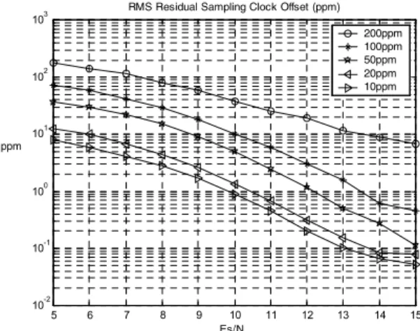
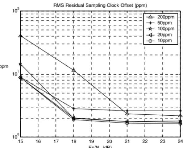
The root-mean-square (RMS) residual sampling clock offset1 is shown in Fig. 1 to Fig.3 for the AWGN, quasi-static frequency-selective, and time-varying frequency-selective fading channels as functions of Es/N0 for

different values of _β, where Es is the average symbol energy

per subcarrier. In Fig. 3 the maximum normalized Doppler-spread of the channel is fmTU = 0.015, which

corresponds to a vehicle speed of 100 km/h. It can be seen that for the frequency-selective fading channels, at high SNR the RMS residual sampling clock offset is less than 2 ppm even when β is as high as 200 ppm.

1 _{This is equal to the RMS sampling clock offset estimation error.}

The channel bit error rate (BER) is plotted as functions of

Es/N0 in Fig. 4 for frequency-selective fading channels with

fmTU = 0 (quasi-static) and fmTU = 0.015. The sampling

clock offset is β = 50 ppm. In each case three receivers are simulated: 1) a receiver that estimates the sampling clock offset using the proposed approach and uses the sinc interpolation for compensation (labeled as “PROPOSED”) ; 2) a receiver with perfect sampling clock offset compensation (labeled as “PERFECT”); and 3) a receiver (labeled as “NO SYNC”) without sampling clock offset compensation in each frame (68 OFDM symbols). All receivers use the same symbol-timing and frequency offset estimation algorithms. It can be seen that, if uncompensated, a sampling clock offset of 50 ppm causes significant degradation in BER. Furthermore, the proposed algorithm is very effective and achieves almost the same performance as the “perfect” case. Finally, the proposed algorithm is robust against Doppler-spread because it achieves roughly the same performance for both values of

fmTU. 5 6 7 8 9 10 11 12 13 14 15 10-2 10-1 100 101 102 103 Es/N 0

RMS Residual Sampling Clock Offset (ppm) 200ppm 100ppm 50ppm 20ppm 10ppm ppm

Fig. 1 RMS residual sampling clock offset (ppm) in AWGN channel.

15 16 17 18 19 20 21 22 23 24 25 10-1 100 101 102 Es/N 0

RMS Residual Sampling Clock Offset (ppm) 200ppm 100ppm 50ppm 20ppm 10ppm ppm

Fig. 2 RMS residual sampling clock offset (ppm) in a frequency selective fading channel without Doppler effect.

15 16 17 18 19 20 21 22 23 24 100 101 102 Es/N 0 (dB)

RMS Residual Sampling Clock Offset (ppm) 200ppm 50ppm 100ppm 20ppm 10ppm ppm

Fig. 3 RMS residual sampling clock offset (ppm) in a frequency selective fading channel with maximum Doppler-spread fmTU = 0.015.

5 10 15 20 25 10-2 10-1 100 E s/N 0 (dB) B ER FADIN G NO SYN C f_mT_u=0.015 FADIIN G NO SYNC fmTu=0 FADIN G PROPOSED f_mT_u=0.015 FADIN G PROPOSED f_mT_u=0 FADIN G PER FEC T f_mT_u=0.015 FADIN G PER FEC T fmTu=0

Fig. 4 BER of perfect sampling clock compensation, the proposed algorithm, and without sampling clock offset compensation

in frequency selective fading channels.

VIII. CONCLUSION

In this paper, we propose a sampling clock offset estimation algorithm using the DVB-T frequency-domain scattered pilot pattern. The algorithm builds upon a least-squares estimator for channel delay and can be used in AWGN or time-varying fading frequency-selective fading channels. Channel estimation or decision feedback tracking loop [2][3] are not required, therefore the proposed algorithm has fairly low complexity. Simulation results show that the proposed algorithm the estimator proposed in this paper is very accurate and robust against multipath fading and Doppler spread, and can reliably estimate the sampling clock offset from 10 ppm to 200 ppm.

REFERENCES

[1] ETSI, “Digital Video Broadcasting: Framing Structure, Channel coding, and Modulation for Digital Terrestrial Television”, European Telecommunication Standard EN300744, Aug. 1997.

[2] Baoguo Yang, Zhengxin Ma, and Zhigang Cao, “ML-Oriented DA Sampling Clock Synchronization for OFDM Systems”, International Conference on

Communication Technology, 2000, Vol.1, pp. 781-784.

[3] Baoguo Yang, K. B. Letaief, Roger S. Cheng, and Zhigang Cao, “An Improved Combined Symbol and Sampling Clock Synchronization Method for OFDM Systems”, IEEE

Wireless Communication and Networking Conference, WCNC, 1999, Vol. 3, pp.1153-1157.

[4] Yong-Jung Kim, Dong-Seog Han and Ki-Bum Kim, “A New Fast Symbol Timing Recovery Algorithm for OFDM Systems”, IEEE Transactions on Consumer Electronics, Vol.44, No.3, pp.1134-1141, August 1998.

[5] P. Dent, G.E. Bottomley, and T. Croft, Jakes fading model revisited,” Electronics Letters, Vol.29, No.13, pp.1162-1163, June 1993.

[6] Richard van Nee, Ramjee Prasad, OFDM for Wireless