THE GENERALIZED RADIAL HILBERT TRANSFORM AND ITS APPLICATIONS TO
2-D EDGE DETECTION (ANY DIRECTION OR SPECIFIED DIRECTIONS)
Soo-Chang Pei,
Jian-Jiun Ding
Department of Electrical Engineering, National Taiwan University, Taipei, Taiwan, R.0.C
Email address:
pei@,cc.ee.ntu.edu.tw
ABSTRACT
It is well-known that the Hilbert transfonn (HLT) is useful for generating the analytic signal, and saving the bandwidth required in communication. However, it is known by less people that the HLT is also a useful tool for edge detection. In this paper, we introduce the generalized radiant Hilbert transform (GRHLT), and illustrate how to use it for edge detection. The GRHLT is the general form of the two-dimensional HLT. Together with some techniques (such as section dividing and shorter impulse re-
sponse modification), we can use the GRHLT to detect the edges of images exactly. Using the GRHLT for edge detection has higher ability of noise immunity than other edge detection algo- rithms. Besides, we can also use the GRHLT for directional edge detection, i.e., detect the edges with certain directions.
1. INTRODUCTION
The Hilbert transform (HLT) is defined as [I]:
OM, (g(x))= IFT(H(0). F T ( g ( x ) ) ) (1)
where H(w) = -j sgn(o). (2)
There are some ways to generalize the HLT into the two- dimensional (2-D) form. The simplest way is combining two I -D HLT's together:
OHIc(2D) Y ) ) = OHIt(,) b H ! t ( x ) ( d . 3 Y))J (3)
gH(X,y)=IFT2D[exp(iPB)FT2D(g(x,Y))l (4) Recently, in [Z], Davis, McNamara, and Cottrell introduced the radial Hilbert transform (RHLT):
where B =cos-'(dR)=sin?(s/R), R = ( ~ + s * ) " ~ , 0, s are the inde- pendent variables in the frequency domain, and P i s any integer.
It is well-known that we can use the HLT to generate the analytic signal, and save the bandwidth required for a real signal. In fact, the HLT can also be applied to edge detection [2][3]. Fewer people know this application, but it is very important. The most serious problem for most of the edge detection algorithms is that their performance is affected by noise. However, using the HLT for edge detection can much rcducc the effects of noise.
In this paper, we introduce the generalized radial Hilbert transform (GRHLT), which is the generalization of the separable 2-D HLT (see (3)) and the RHLT (see (4)). We introduce it in
Sec. 2. Then, we illustrate how to use the GRHLT for 2-D edge detection and its advantage in Sec. 3. The most important two advantages are noise immunity and that the ramp edges can be detected successfully. Using the GRHLT together with the tech- niques introduced in Sec. 4, we can detect the edges of an image exactly. Besides, in Sec. 5 , we will show that we can also use the
GRHLT for directional edge detection, i.e., detect the edges with certain directions.
2. GENERALIZED RADIAL HILBERT TRANS- FORMS
We define the generalized radial Hilbert transform (GRHLT) as follows:
gH
(&
Y ) = I F T ~ D (H(0, SIFT20k(&
Y ) ) ) ( 5 ) ( 6 )where the transfer function H( o,s) is rotational symmetric:
H(w,
s) = O(B) when (a, s) # 0, H(0,O) = 0 , where 8 = cos-' (0 / r ) = sin? (s / r ),
r =
dW2+S2,
o(@
is any function. (7)The separable 2-D HLT defined as in (3) is a special case of the GRHLT where @(8) = 1 when 0 < B < ni2 or z< B < 3ni2,O(@
= -1 when ai2 < B < z or 3 d 2 < l?< 2z. and Q ( 9 = 0 when B
= Nd2. The RHLT introduced in [2] is a special case of the GRHLT where
O(@ =exp(iPB). (8)
Besides, many other operations (such as the analytic signals generating operations, the I-D HLT, and identity operation) are
also the special cases of the GRHLT.
The GRHLT is very general and flexible. Because of its flexibility, it can solve many problems that can't be solved well by its special cas& In Secs. 3-5, we show that the GRHLT is a very powerful tool for edge detection.
When doing the edge detection, we usually use the discrete counterpart of the GRHLT, i.e., the discrete generalized radial Hilbert transform:
where p, q, are the discrete independent variables in the fre- quency domain, and H(p, q] is rotational symmetric:
S H [M,"1=IDFT,D(H[p,91DFT,,(g[m,nl)) (9)
H [ p , q ] =
@(e)
H[O,O]=O,
H [ M / Z , O ] = O
ifMiseven, H[O, N / 2]= 0 B=cos-] ( p i . ) =
sin+(q/ r ) , whcn [p, q1 f 10, 01,i f N i s even, (MxN the size ofg[m, n]),
r =
Q(4) is any function. (10)
Due to the DFT and IDFT, the discrete generalized radial Hil- bert transform has fast algorithm. Its complexity is MN.lag2MN.
3. USING THE GRHLT FOR EDGE DETECTION
The simplest way for 2-D edge detection is doing the difference operation. That is, if
(horizontal) Ig[mo,no]-g[m,,no
+Ill
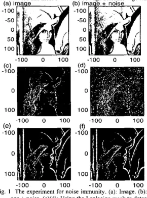
>threshold (vertical) Ig[m,,no]-g[mo +I,n,]l >threshold (1 I ) we can conclude that the pixel (mo, no) is on the edge. Besides, there are also some edge detection methods based on the convo- lution with 3x3 matrix, e. g., the compass gradient mask, Lapla- cian mask, and statistical mask methods [4]. Their ideas are simi- lar to the difference operation.However, most of the above edge detection methods are highly influenced by noise. We do an experiment in Fig. 1. Fig. l(a) is the input image, and Fig. I(h) is the image interfered by the noise. In Fig. I(c), I(d), we use the Laplacian mask method to detect the edges of Fig. I(a), I(b), respectively. It is appear- ance that the effect of the Laplacian mask method is much influ- enced by noise. This is the most important problem for Laplaciau mask method and most of the existed edee detection aleorithms.
. . .
(a) i -100 -50 0 50 100 -100 0 100 -100 0 100 ( C ) (d) -100 -100 0 0 100 100 -100 0 100 -100 0 100 -100 0 100 -100 0 100 Fig. I The experiment for noise immunity. (a): Image. (b): Im-
age +noise. (c)(d): Using the Laplaciau mask to detect the edges of (a) and (b). (e)(f): Using the GRHLT to detect the edges of (a) and (b).
However, if we use the GRHLT for edge detection, we can much reduce the effect of noise.
In (IO), if the transfer function we choose satisfies
@(B)
=4 ( 0
+
z)
for all8,
('2)we can use the GRHLT far 2-D edge detection. This is so be- cause in this case the impulse response (denoted by h[m, n] =
IDFT(H[o, s]) of the GRHLT has the following two properties: ( I ) odd symmetric: h[m, n ] = -A[-m, -n],
(2) lh[m, n]l has the trend ofbecoming smaller when Iml, In1 grow larger.
In fact, except for the GRHLT, all the 2-D LTI operations whose impulse responses satisfy the above hvo constraints can also be used for edge detection.
The GRHLT can much reduce the effect of noise because it has longer impulse response. The impulse response of the differ- ence method (see (11)) are [-I, I] or [-I, 1IT. Their lengths are
1x2 and 2x1. The impulse responses of the methods based on
3x3 matrix convolution (such as the Laplacian mask method) are
3x3. However, the GRHLT has much longer impulse response, so it can reduce the effect of noise. In Fig. I(e) and I(f), we do the GRHLT for Fig. I(a) and I(b), respectively. Fig. l(e) shows that we can use the GRHLT to detect an image successfully. In Fig.
I(0,
we show that even if the original image is interfered by noise, the performance of edge detection doesn't become worse. So using the GRHLT for edge detection is noise immunity.Besides, ifO(S, satisfies
a@)=
50,
(13)then the GRHLT has the property of real-input-real-output. That is, if the input g [ m , n] is real, then the output gH[m, n] of the GRHLT is also a real function. If we use the RHLT (see (4)), i.e.,
Q(8) = expo@, although it has good performance in edge detec- tion, for real input, the output may not be real since Q(@ =
expo@ doesn't satisfy (13). We can try to choose Q(@ to satisfy (12)and(l3).Forexample,wecanchoone0(6'~as:
O(S)=
j s g n ( c 0 s ( 8 - z / 6 ) ) c o s ~ ~ ~ ( B - z / / ) .
(14)In this case,
O(@
satisfy (12) and (13), and the corresponding GRHLT has the property of real-input-real-output.The advantages of using the GRHLT for edge detection are: ( I ) Noise immunity.
(2) Ramp edges, which are hard to detect by other edge detection
(3) In the sense of sight, the output has better quality
if
we useThe 2"' and 3d advantages can be seen from the comparison of Fig. l(e) with Fig. I(c).
algorithms, can be detected by the GRHLT.
the GRHLT for edge detection.
4. SOME TECHNIQGES
TO
IMPROVE THE PER- FORMANCEOF
EDGE DETECTION4.1. D i v i d i n g t h e i n p u t i n t o s e v e r a l sections
We like to divide the input image into several sections, and use each of them as the input of the GRHLT for edge detection. It has two advantages: (1) The complexity can be reduced. (2) The performance can be improved.
Since the GRHLT is implemented by the 2 - 0 DFT / IDFT, so its complexity is MN.log,MN where MxN is the size of image. If we divide the image into
9
sections, then the size of each sec- tion is near to (M/S)x(N/X) So the complexity becomesMN MN MN
S 2 ~ - l o g 2 ~ = M N l o g 2 ~
S 2
SThis is smaller than MN.log2MN, so the complexity is reduced. We can also write (15) as a function of MoxNo = (M/Sjx(N/S) where &xN0 is the size of each section:
MN log, M,N, (16)
That is, if the size of sections MoxNo is fixed, the complexity grows linearly with MxN. Thus, although the edge detection
algorithm using GRHLT seems more complicated than other edge detection algorithms, if we use the section-division method, the complexity is in fact O(MN). This is the same as the com-
plexities of other edge detection algorithms.
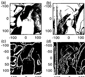
Besides, the performance can also be improved if we divide the input into several sections. This is so because, to conclude whether a pixel is on the edge, we just require the information surrounding the pixel. It is unnecessary to use the whole image as the input of the GRHLT for edge detection. In Fig. 2, we do some experiments. In Fig. 2(b), we don’t divide the image, and in Fig. 2(c)(d), we divide the image into 3’ and 9’ sections before using the GRHLT for edge detection. We can see that, in Fig 2(c)(d), the brightness differences between edee reeions and
where Z , [m, n ] = lg, [m, n] @ A,
,
A c is a cxc matrix where A,(m, n ) = I for all m’s, n’s,
In the above, there’re 3 parameters a, b, c. We can adjust them to
achieve better performance. In principle, for a simple image (such as the fruit image in Fig. 3(a)), we choose larger values of a and c and smaller value of b. For a complicated image (such as the Lena image in Fig. 3(b)), we choose smaller value of a and c and larger value of b. In Fig. 3(c), we choose (a, b, c) as (0.65, 0.8, 15), and in Fig. 3(d), we choose ( a , b, c) as (0.5, 0.85,9).
TO is the average value of b [ m , n]l. (20)
-
-non-edge regions are more obvious than that in,Fig. 2(b).
-1
‘bb
0(a)
-1 00 0 0 100 100 -100 0 100 -100 0 100 -100 0 100 -100 0 100Fig. 2 Improving the performance of the GRHLT for edge de- tection by section-division method. (a) Image. (b) The IC-
sults if we do not separate the input. (c)(d) The results if we separate the input into 3’ sections and 9’ sections.
4.2. Appending tapered borders
When doing edge detection, the borders of an image are usually misunderstood as the edges. This problem can be overcome by appending tapered borders to the original image before doing the edges detection. That is, if the original image is g[m, n ] where 1-N, i m , n
<
N-NI, NI = [N/Z]+l, then we can append the up- per and lower tapered borders to g [ m , n] by:g[m,nl= (m+B-I+N,)g[l-Nl, n]/B when 2-AJ-B 9 n <I-N,,
g [ m , n ] = ( N + N , + B - m ) g [ N ~ N , , ~ ] / B when N-N,im< N+N,+B-l
We can use the similar way to append the left and right tapered borders to g[m, n ] . AAer appending tapered borders, the borders of an image are no longer detected as edges.
4.3. Choosing the adaptive threshold
In Figs. I , 2, we directly show the output oftbe GRHLT. In fact, we can also choose a threshold. If
(17)
( g , [ m , , n o ] (
>
threshold (18) where g,,[m, n] is the output of the GRHLT, then we can con- clude (mo, no) is on an edge. Then, one may ask how to choose the threshold. The simplest way is choosing the threshold assome constant. However, it has worse performance for a compli- cated image. Here, we propose an localized and adaptive method to choose the threshold function n m , n ] :
-100 0 100 -100 0 100 (C) ( d ) -100 -100 -50 -50 0 0 50 50 100 100 -100 0 100 -100 0 100
Fie. I 3 Edee detection usinn the GRHLT toeether with the adao-
tive threshold funccon defined as in719), (20).
4.4.
Shorter impulse response modificationWe have stated that the advantage of the GRHLT is that it can reduce the effects of noise. It is mainly due to the GRHLT has longer impulse response. However, it has some side effect. That is, the result is not sharp enough, and sometimes the brightness of the edges region may not be obviously higher than the bright- ness of the non-edge regions. This problem can be overcome if we modify the transfer function of the GRHLT a little. We can modify the transfer function of the GRHLT in (1 0) as:
where @ is circular convolution, A , is a dxd mamx, A d m , n ) = 1 for all m’s, E ’ S , and O(@J is defined the same as previous sec- tions. If c is larger, the impulse response hd[m, n ] = IDFT(H&,
y]) will become shorter. Shorter impulse response makes the brightness difference between the edge regions and the non-edge regions become more obvious.
In Fig. 4, we do some experiments. In Fig. 4(a)(c), we show the slicing (along x-axis) of the impulse response of the original GRHLT and the modified GRHLT (d = 9). It can be seen that the impulse response of the modified GRHLT becomes shorter. Then, in Fig. 4(b)(d), we show the transform results of the origi- nal GRHLT and modified GRHLT, respectively. The brightness difference between the edge and the non-edge regions of the result of the modified GRHLT is more obvious.
Thus, using the shorter impulse response GRHLT for edge detection can obtain better performance. However, the ability of noise immunity is reduced. There is a tradeoff between the two
H d [ P > q l = @ ( Q ) @ A d , (21)
goals: (I) better performance of edge detection, (2) higher ability for noise immunitv.
-50 0 50 100 O b .... -
__-..
-0.5 -1 0 0 10 -100 0 100 (d) -100 -50 0 50 100 -0.51-
-1 .. n 0 i n .. -inn n inn Fig. 4 Experiments for using the shorter impulse response modi-fied GRHLT for edge detection. (a)(b) The impulse response (x-axis slicing) and the transform results of the original GRHLT. (c)(d) The impulse response and he transform re- sults of the shorter impulse response modified GRHLT.
5. DIRECTIONAL EDGE DETECTION
In Secs. 3,4, we detect the edges whatever the direction it has. In
fact, if the transfer function of the GRHLT is chosen properly, we can detect the edges with certain directions. For example, If we want to detect the edges with the direction in the region of [#,,
41
where4-4,
< n, then, in (IO), we can choose@(@ = j when # , - d B <4-n,
Then we do the GRHLT. If the output r&m,n)l > threshold, then we can conclude that ( m , n) is an an edge, and the direction of the edge is in the range of [+,, 41. In Fig. 5 , we give some ex- ample. We use a circle (Fig. 8(a)) and the Lena image (Fig. 8(b))
as the input. In Fig. 5 ( c ) , we plot the imaginary part of the trans- fer function
&,
q ] = O ( @ , wherea(@
is defined as (22). Here, we choose (I = d3 and4
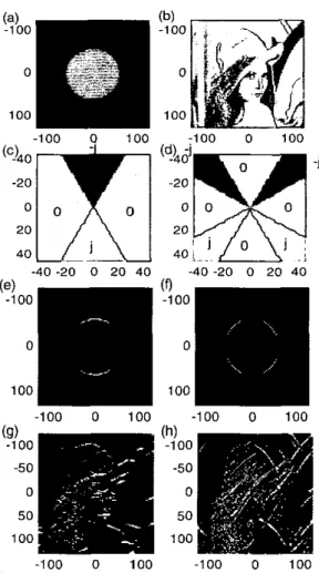
= 2 d 3 . Then we do the GRHLT for the two inputs, and use the method described in subsection 4.3 to choose the adaptive threshold. We plot the transform results in Fig. 8(e) and 8(g). The edges found in Fig. 8(e) are just two arcs, and the angle ranges of the two arcs are [d3, 2 d 3 ] and [-m’3,d3], respectively. In Fig. 5(g), we also find the edges with direc- tion in the range of [ d 3 , 2 d 3 ] successfully.
Besides, i f w e want to detect the edges in the region of [#,,
41
and[4,
4
at the same time, we can choose O ( @ as:when (, i B i
h,
h
5 B id4,
when
#,-x<
.9 54-z,
h-n<
B
2k-n,
For example, in Fig. 8(d), we choose
4l
= [d6. “31, and choose[4,
rj4] = [ 2 d 3 , 5461. In Fig. 5(f) and 5(h), we plot the transfer results of the GRHLT (with threshold) with this transfer function for the circle image and Lena image. We detect the edges with the direction in the ranges of [ d 6 , ”31 and [ 2 d 3 , 8 d 6 1 successfully.Thus, using the GRHLT for directional edge detection is very flexible and convenient.
@(@ = -j when
4,
i B S4,
@(@ = 0 othenvise. ( 2 2 ) O(B) = -j @(@ = j O ( @ = 0 otherwise. (23) (b) -1 00(a)
-100 0 0 100 100 -100a
100 -100 0 100 4 O I / - j \ [ 4 0 ; ~i i / o
- 4 0 - 2 0 0 20 40 -40-20 0 -100 0 100 -100 0 100(hl
-100 -50 -50 0 0 50 50 100 100(9)
.loo -100 0 100 -100 0 100Fig. 5 Experiments for directional edge detection. (a)(b): The inputs. (c)(d): Transfer functions
a(@.
(e)(g): The trans-form results if we use (c) as the transfer function. (f)(h) The transform results if we use (d) as the transfer function.
6. CONCLUSION
We have introduced the generalized radiant Hilbert transform (GRHLT), and illustrated how to use it for 2-D edge detection. Using the GRHLT for edge detection is very flexible, and can much reduce the effect of noise. We can even use the GRHLT for directional edge detection. Thus, except for communication, the GRHLT is also an important tool for image processing.
7.
REFERENCES
[ I ] S. C. Hahn, Hilbert Transforms in Signal Processing, Boston: Anect House, 1996.
[2] J. A. Davis,
D.
E. McNamara, and Don M. Cottrell, “Image processing with the radial Hilbert transform theory and experi- ments”, Opt. Lett., vol. 28, p. 99-101, Jan. 2000.[3] A. W. Lohmann,
D.
Mendlovic, and Z. Zalevsky, “Fractional Hilbert transform”, Opt. Lett., vol. 21, p 281-283, Feb. 1996.[4] Pratt, William K, Digitd image processing, 3‘d Ed., New York: Wiley, 2001.