多媒體影音高階處理、傳輸及設計－總計畫:多媒體影音高階處理、傳輸及設計(3/3)

行政院國家科學委員會專題研究計畫 成果報告

多媒體影音高階處理、傳輸及設計--總計畫:多媒體影音高

階處理、傳輸及設計(3/3)

研究成果報告(完整版)

計 畫 類 別 ： 整合型

計 畫 編 號 ： NSC 96-2221-E-002-088-

執 行 期 間 ： 96 年 08 月 01 日至 97 年 07 月 31 日

執 行 單 位 ： 國立臺灣大學電機工程學系暨研究所

計 畫 主 持 人 ： 貝蘇章

共 同 主 持 人 ： 陳良基、李枝宏、馮世邁、貝蘇章

計畫參與人員： 教授-主持人(含共同主持人)：貝蘇章

學士-專任助理人員：王光絢

報 告 附 件 ： 出席國際會議研究心得報告及發表論文

處 理 方 式 ： 本計畫可公開查詢

中 華 民 國 97 年 06 月 05 日

多媒體影音高階處理、傳輸及設計--總計畫 (3/3)

Multimedia Audio/Video High Level Processing,

Transmission and Design (III)

計畫編號: NSC 96-2221-E-002-088

執行期限：96 年 8 月 1 日至 97 年 7 月 31 日

主持人：貝蘇章 台灣大學電機系教授

摘要 在智慧型視訊及影像分析，人臉偵測及辨識將是重 要課題，膚色將是一個非常重要而且有效的臉部特 徵可以應用，本論文探討人類膚色的彩色空間分佈 圖，同時進一步分析白種，黃種及黑種人類膚色的 彩色區域分布，並進行不同人種的偵測及辨識。 ABSTRACT

With the growing technique of communication between human and robot, the problem of human face recognition has attached more importance and become the current research in the popular domain of computer vision and recognition model. Thus, human’s skin color is always an important mechanism and principle basis of human face detection. Human’s skin color has the relative stability with the difference of the majority background object appearance. The skin color does not rely on the face detail characteristic and do not change with the face expression and rotation. Therefore, utilizing skin color to examine human face in color image is an important context of human face recognition.

In this paper, we provide a fast algorithm to identify human race with face skin color. The basic construction is roughly dividing human race into three parts: white, yellow and black race, then using Gaussian Mixture Model to train the feature parameter of each human race with large number of training images. Afterward, utilize Bayesian Decision Rule to determine the human race of test images.

1. INTRODUCTION

Face detection techniques based on the use of color information have been proposed recently. Take into account that the major dissimilarities between different races of people who have different skin color lie mostly in their chrominance so that skin color can be considered as good face segmentation and racial recognition feature. The main advantage in

segmentation and racial recognition through the color characteristics is that facial detection can be performed independently on the size, position and expression of the face within the image. Also using color characteristics to classify human race is more convenient than using facial feature.

In our proposed method, we classify human races into three typical categories: white, yellow and black people (or Caucasian, Mongoloid and Negroid). First, several images are trained to get parameters of each race with GMM analysis. According to the analysis of GMM, there are tiny differences among these parameters of three different races and we use these parameters to classify the racial category of each testing image. We gathered the statistical result and displayed the experiment consequence in section 5.

2. HUMAN SKIN COLOR DISTRIBUTION 2.1 YCbCr color space

The formula between RGB and YCbCr is list below:

16

0.257

0.504

0.098

128

0.148

0.291

0.439

128

0.439

0.368

0.071

Y

R

Cb

G

Cr

B

  

 

  

  

₌

 

_{+ −}

₋

  

  

 

  

  

 

−

−

  

  

 

  

According to [1], most skin color pixels distribution and boundary box in the Cb-Cr plane show in Fig 1. The ranges of boundary box are:76≤Cb≤124

Fig 1.Skin color distribution and boundary box in CbCr color space in Ref [1].

Considering only color information, a pixel will be classified as skin if both of its color components are within each of these ranges. So, the technique used for the racial recognition and face segmentation consists of defining maximum and minimum thresholds for each of the two chromatic components.

2.2 YCgCr color space

There is another useful color coordinate: YCgCr, a novel color space based on YCbCr, was mainly proposed in [1, 2] for face segmentation. It is based on YCbCr, but it differs on the use of the Cg color component instead of Cb. The color spaces used in television systems (YUV, YCbCr) are transmission oriented, so in order to minimize the encoding decoding errors, they use the biggest color differences: (R-Y) and (B-Y). The YCgCr color uses the smallest color difference (G-Y) instead of (B-Y).

The YCgCr components can be obtained in a similar way than the YCbCr equations described in the ITU Rec. BT. 601 and expressed in terms of Y’, G’-Y’, R’-Y’ components defined in the [0,1] range using the following matrix expression:

16

219

'

Y

= +

×

Y

,

'

0.299

' 0.413

' 0.144

'

Y

=

× +

R

× −

G

×

B

...Eq(1)

1

128 112 [

( '

')]

1 0.587

Cg

=

+

×

G

−

Y

−

………Eq(2)

1

128 112 [

( '

')]

1 0.299

Cr

=

+

×

R

−

Y

−

……….Eq(3)

Luminance and chrominance are coded in 8 bits. Y has an range of 219 and an offset of 16. The chromatic components are defined in the rage [16,240], with range of

±

112 and an offset of 128. Each component is coded in 8 bits. Expressed in matrix form, R’G’B’ components can be easily transformed to YCgCr components: 16 0.257 0.504 0.098 128 0.316 0.439 0.121 128 0.439 0.368 0.071 Y R Cg G Cr B           ₌  _{+ − −}                 − −            …..Eq(4)

According to [2], most skin pixel color distribution can be detected in the chrominance bounding box in CgCr domain shown in Fig 11. A pixel will be considered as skin if both of its color components are within each of the ranges defined by the maximum and minimum thresholds of the

chrominance plane coordinates Cg and Cr. Where (Cg min, Cg max)=[76, 125] and (Cr min, Cr max)=[136, 202].

Fig 2.Skin color distribution and boundary box in CgCr color space in Ref[2].

Consider the skin color distribution depicted in Fig 2, it is possible to achieve a better performance of the face segmentation in the YCgCr color space by defining a boundary box in the direction of the line that connects the Red and Cyan colors, where most of the skin values are concentrated.

New decision thresholds constituting a nonrectangular region (the black region inside the boundary box shown in Fig 2) can be defined, so that the Cr thresholds are the same vertical limits of the boundary box, while the Cg thresholds, Cg min and Cg max lines, are parallel to the Red-Cyan line. Hence the Cr min and Cr max thresholds and the Cg min and Cg max lines, according to the following equations:

min max Cr ≤Cr≤Cr …………..…….Eq(5) (Cr min, Cr max)= [136, 202]. (305 ) min 1.38 max 1.38 1.38 Cr Cr Cr Cr Cg − _{≤ ≤} + × − _Eq(6)

Instead of using two binary masks for face segmentation based on the Cg and Cr thresholds of the boundary box, in the case of a nonrectangular decision region, for every Cr value, a binary mask is used for each Cg min and Cg max pair of Cg thresholds. The final mask for face segmentation is obtained as the intersection of all the binary masks.

2.3 The reasons of choosing YCgCr

The black cluster of Fig 1 and 2 represent the majority of human skin chrominance in different domains. Fig 1 displays human skin chrominance of CbCr and Fig2 represents that of CgCr. Compare Fig 1 to Fig 2, the shape of black cluster of Fig 2 in CgCr domain is more regular than that of Fig 1. The human

skin distribution in CgCr is less widespread than that in CbCr and more centralized as ellipse shape.

Because the chromatic distribution of CgCr has better shape than that of CbCr, it will achieve better performance in GMM detection. The slanted thin ellipse shape in CgCr domain means the negative correlation between Cg and Cr. The large value of Cg results in small value of Cr so that Cg and Cr have strong correlation.

Contrariwise, the relation between Cb and Cr displays a random-like distribution in Fig 1 and the shape is more widespread so that it is more difficult to analyze the distribution in CbCr domain.

2.4 Distribution in YCgCr domain of different races

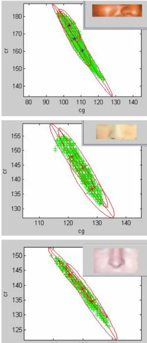
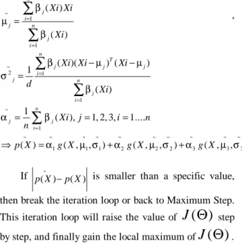
We use YCgCr domain to compute our experiment with GMM analysis of different races’ pictures which only include the region of nose, because this region is purity of skin color without the effects on other colors of lip or eyes. There are three typical human races (white, yellow and black (or Caucasian, Mongoloid and Negroid)) and their distribution of CgCr domain shown in Fig 3.

. .

Fig 3.Different racial color distribution in CgCr domain We choose three typical pictures to represent each racial distribution of CgCr shown in Fig 3. The red cluster displays Caucasian’s distribution in CgCr domain, the blue region displays Negroid’s distribution and the yellow cluster displays Mongoloid’s. It can be seen that the majority of black people’s distribution are at the location between white people and yellow people. Also the Mongoloid’s distribution has larger value in CgCr domain than others while he Caucasian’s distribution has smallest value in CgCr domain.

2.5 Brightness and other chromatic distribution

There are several other kinds of color coordinates to represent the distribution with different races. The researches on Lab and Yuv represented in [3,4] show

that Negroid has less brightness than Caucasian and Mongoloid.

Fig 4. Saturation and brightness chromatic distribution of flesh tone in Ref [3][4] (a) uv; (b) La chromaticity

In Fig 4(b), Caucasian has greater brightness value than other races and in (a), saturation value which is represented to the magnitude of u and v is distributed greatly to Negroid, but the hue value which is represented to the angle of u and v is almost same for races. Thus, the flesh tones for races are discriminated for the combination value of both saturation and brightness.

Fig 5.Skin color distribution in YCg and Y Cr domain. In Fig 5, there are two figures which show the experiment result of distributions in Y-Cg and Y-Cr domain. They show that Negroid really has less brightness than Caucasian and Mongoloid. Furthermore, Mongoloid has the widest distribution of luminance; we will consider the effect of illumination in GMM analysis.

3. GAUSSIAN MIXTURE MODEL

GMM (Gaussian mixture model) which is the extension of single model Gaussian probability function is a conventional method to analyze non-uniform distributed data and is among the most statistically mature methods for clustering (though they are also used intensively for density estimation. In this tutorial, we introduce the concept of clustering, and see how one form of clustering in which we assume that individual data points are generated by first choosing one of a set of multivariate Gaussians and then sampling from them can be a well-defined computational operation.

Mixture models are a semi-parametric alternative to non-parametric histograms (which can also be used as densities) and provide greater flexibility and precision in modeling the underlying statistics of sample data. They are able to smooth over gaps resulting from sparse sample data and provide tighter constraints in assigning object membership to color-space regions. Such precision is necessary to obtain the best results of optimum means, covariance and weighting possible from color-based pixel classification for qualitative segmentation requirements.

We then see how to learn such a thing from data, and we discover that an optimization approach not used in any of the previous Andrew Tutorials can help considerably here. This optimization method is called Expectation Maximization (EM). We'll spend some time giving a few high level explanations and demonstrations of EM, which turns out to be valuable for many other algorithms beyond Gaussian Mixture Models.

1-D data for example in Fig 6, we can see that 2-3 clusters occupy separate sub-space and the probability of mixture clusters reveals Gaussian like distribution. We can use EM algorithm to find out optimum mean, co variance and weighting value of each cluster. 2-D data for example in Fig 7 also can be estimated by EM algorithm.

Fig 6. The compare of original 1-D data and GMM fitted. (a)The fitting 2 components of GMM. (b) The fitting 3 components of GMM.

Fig 7.2D data with 3-components of GMM fitted We applied 3-components Gaussian mixture models to the cluster of each race, Fig 8 for example. Each component of Gaussian model has its optimum mean, covariance and weighting which are obtained by EM algorithm.

Fig 8. The compare of original 2-D data and GMM fitted with different races. (a)Negroid (b) Mongoloid (c) Caucasian.

3.1 Mixture Gaussian model with EM algorithm

If the shape of these data points’ distribution is not like ellipse in d- dimension, then we can not use single Gaussian model to describe the probability density function of these data points. So we use several Gaussian distributions with weighted average to describe it, Take 3-components GMM for example, the probability density function can be expressed as:

1 1 1 2 2 2 3 3 3 ( ) ( , , ) ( , , ) ( , , ) p X =αg X µ Σ +α g X µ Σ +α g X µ Σ 1g1 2g2 3g3 α α α = + +

There are several parameters of this density function (α µ_{1 1},Σ₁,α µ_{2 2},Σ₂,α µ_{3 3},Σ₃ ), and there is a condition ofα α α₁, ₂, ₃:

1, 2 3 1

α α α+ + =

The kind of expression is called GMM. In order to simply the calculation, we let the covariance matrix of each Gaussian density function become: 2

j σjIdxd Σ = . So 2 2 ( ) ( ) 1 1 ( , , ) exp( ) 2 2 (2 ) T j j j j d d j j X X g X µ σ µ µ σ π σ − − = − Let (

α µ

1 1

,

Σ

1

,

α µ

2 2

,

Σ

2

,

α µ

3 3

,

Σ

3) =

Θ

, we use EM algorithm to find optimumΘ.

▪ Estimation Step:

1. Define the initial value of

Θ

= (

α µ σ α µ σ α µ σ

_{1 1}

,

₁

,

_{2 2}

,

₂

,

_{3 3}

,

₃ ). We set

1 2 3

1

3

α

=

α

=

α

=

and use k-means to calculate the three centers of the cluster as (

µ µ µ

₁

,

₂

,

₃ ). Initial 2 2 2 2 1 2 3 1 ( ) ( ) 1 T j Xi j Xi j n σ =σ =σ =σ = −µ −µ − .

2. Use these initial parameters to calculateβ₁(Xi),β₂(Xi),β₃(Xi), i=1~n.

▪ Maximum Step:

1. Calculate new parameters with iteration loop. ~ 1 1 ( ) ( ) n j i j n j i Xi Xi Xi β µ β = = =

∑

∑

, ~ 2 1 1 ( )( ) ( ) 1 ( ) n T j j j i j n j i Xi Xi Xi d Xi β µ µ σ β = = − − =

∑

∑

~ 1 1 ( ), 1, 2, 3, 1.... n j j i Xi j i n n α β = =

∑

= = ~ ~ ~ ~ ~ ~ ~ ~ ~ ~ 1 1 1 2 2 2 3 3 3 ( ) ( , , ) ( , , ) ( , , ) p X α g X µ σ α g X µ σ α g X µ σ ⇒ = + +

If _{p X(}~ _{)−p X( )} is smaller than a specific value, then break the iteration loop or back to Maximum Step. This iteration loop will raise the value of

J

( )

Θ

step by step, and finally gain the local maximum of

J

( )

Θ

.

4. CLASSIFICATION RULE

In this section the Bayesian Theory is used to derive a decision machine (classifier) used in a verification system. The machine is then implemented using GMM approach. The k-means, EM algorithm and maximum a posteriori (MAP) adaptation algorithm, used for finding GMM parameters, are described. The section is concluded by a discussion on implementation issues.

4.1 Bayesian Decision Theory

A verification system, on the fundamental level is a two- class decision machine: based on given observation vectors, the client is either an impostor or the true claimant. In this section we shall use Bayesian Decision Theory [7] to implement the decision machine. Let us denote client specific true claimant and impostor classes as C1 and C2 respectively, and let

[ 1....

]

T

x

x

xn

→

=

be the observation vector. Moreover, let P(Cj) be the a priori probability of class Cj, and P(

x

→

| Cj ) be the conditional probability density function (pdf) of

x

→

, given class Cj. We seek to find the class that

x

→

belongs to. Using the Bayes formula [9], we obtain: ( | ) ( ) ( | ) ( ) P x Cj P Cj P Cj x P x → → → = , where 2 1 ( ) ( | ) ( ) i P x P x Ci P Ci → → =

Thus using the Bayes formula we obtain the a posteriori probability of Cj, j=1, 2. It follows that the Bayes decision rule is then:

Choose C1 if P C( 1 | )→x >P C( 2 | )→x

Or more generally, index of chosen class =

arg max ( | )

j P Cj x

→

which is known as the maximum a posteriori decision rule. It must be noted that p(x) is not required for making the decision. Thus the decision rule becomes:

arg max ( | ) ( )

j P x Cj P Cj

→

.

Intuitively, the decision machine will make fewer mistakes when using more observations vectors. Thus in practice, multiple observation vectors are used: X= xi, i=1…n. Assuming that the observation vectors are independent and identically distributed (iid), then the joint likelihood is:

1 ( | ) ( | ) ( ) n i i P X Cj P x Cj P Cj = → =

∏

.

In practice, the true form of the pdf P X Cj( | ) is unknown, hence a parametric representation,P X Cj~( | ), estimated from training data, is used instead. Since

~

( | )

P X Cj is only an approximation, a correction

function, P X Cj≈( | ), is required. ~ 1 ( | ) ( | ) ( | ) ( ) n i i i P X C j P x C j P≈ x C j P C j = → → =

∏

Taking into account the multiple observation vectors and rewriting _{arg max ( | ) ( )}

j P Cj x P Cj → into ratio test yields: Choose class = ~ ~ ~ ~ ( | 1) ( | 2) ( 2) 1 ( | 2) ( | 1) ( 1) ( | 1) ( | 2) ( 2) 2 ( | 2) ( | 1) ( 1) P X C P X C P C C if P X C P X C P C P X C P X C P C C if P X C P X C P C ≈ ≈ ≈ ≈ > <

Due to precision issues in computational implementation, it is more convenient to use a summation rather than series of multiplications. Since log(.) is a monotonically increasing function, the decision rule can be modified to:

Choose class = ~ ~ ( | 1) ( | 2) ( 2) 1 log( ) log( ) ( | 2) ( | 1) ( 1) 2 P X C P X C P C C if P X C P X C P C C if others ≈ ≈ >

which translates to:

Choose class = ~ ~ _{( | 2) ( 2)} 1 log( ( | 1)) ( ( | 2)) log( ) ( | 1) ( 1) 2 P X C P C C if P X C log P X C P X C P C C if others ≈ ≈ − >

Where, for clarity, ~ ~

1 log ( | ) log ( | ) n i i P X Cj P x Cj = → =

∑

Due to practical considerations described later, the number of observation vectors needs to be taken account. Choose class = ~ ~ 1 1 ( | 2) ( 2) 1 [log( ( | 1)) ( ( | 2)] log( ) ( | 1) ( 1) 2 P X C P C C if P X C log P X C n n _{P X C P C} C if others ≈ ≈ − > Let us define ~ ~ 1 1 ( | ) log( ( | )) log( ( | )) n i n L X Cj P X Cj P x i Cj n n → = = =

∑

This can be interpreted as the average log likelihood of X. Thus we can choose class =

1 ( | 2) ( 2) 1 ( | 1) ( | 2) log( ) ( | 1) ( 1) 2 P X C P C C if L X C L X C n _{P X C P C} C if others ≈ ≈ − > Let us define

Λ

( )

x

=

L X C

(

| 1)

−

L X C

(

|

2)

Since the true form of the pdf p(x|Cj) is unknown, the correction function, P X Cj( | )

≈

, is also unknown; moreover, in real life situations the a priori probabilities P(C1) and P(C2) are often unknown. Thus in practice, 1 ( | 2) ( 2) log( ) ( | 1) ( 1) P X C P C n _{P X C P C} ≈ ≈ is replaced with an experimentally found threshold, t.

Choose class = 1 ( )

2

C if x t

C if others

Λ > _{, t=0, usually.}

Strictly speaking, the normalization factor 1/n is not necessary to make a decision. However, in practical situations variable length observations are often encountered. Since Λ( )x is observation length independent, it allows the approximation of the distributions of Λ( )x for true clients and known impostors, which in turn simplifies the selection of the threshold.

We first calculate 3-components GMM parameters of each race in every two of three color space and average-normalize those means, covariance and average weightings of each training image, then put testing images into Bayesian Classification Rule to find max P(X|Cj),j=1,2,3 in two of three color space and make decision with majority of voting result.

If the majority of voting result is correct, then we said that it is an accurate detection. If the majority of voting result is not correct, then we call it is an error detection.

Result of Uncertainty will also be discussed. There are several conditions to result in uncertainty.

1.When the voting results of two of three color spaces are equal, for example, if decision is Caucasian in YCg, Mongoloid in YCr and Negroid in CgCr, then it will be an uncertainty.

2.If | P(X|Cj)- P(X|Ci)|<t, i≠j, i,j=1,2,3 in any two of three color spaces, it is also an uncertainty.

Usually the tiny distinction of P(X|Cj) among three race categories are unable to make decision by the voting result.

5. EXPERIMENT RESULT

We collect two sets of three races pictures, each race of every set includes about more than 15 training images and more than 30 testing images, these pictures in two sets are all distinct. These pictures are collected from several face image databases on internet and web albums of daily life. So the training images and testing images include many different kinds of picturing situations such as different luminance condition, night model with flashlight, daytime model with much exposure.

We use two of three YCgCr domains to compute our experiment with GMM analysis of different races’ pictures which only include the region of nose, because this region is purity of skin color without the effects on

other colors of lip or eyes. So we cut each full-face picture into region with noise.

We use MATLAB 6.5 to implement the experiment and count accuracy, error rate and uncertainty of these two sets of experiment and we will discuss result in the following sections.

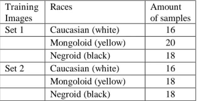
Training Images

Races Amount

of samples Set 1 Caucasian (white) 16

Mongoloid (yellow) 20 Negroid (black) 18 Set 2 Caucasian (white) 16 Mongoloid (yellow) 18 Negroid (black) 18

Table 1 : Amount of Training images in Set 1 and Set 2

Table 2 : Classified Accuracy of each race in Set 1

Table 3: Classified Accuracy of each race in Set 2

5.1Discussion on false detection

According to the result, we can see that the accuracy of Negroid is the lowest; this is because the distribution of Negroid in CgCr domain shown in Fig 3 is between Caucasian and Mongoloid. This kind of distribution may result in the false judgment easily and lead to low accuracy. Testing Images Races Amount of samples Accuracy Erro r rate Uncertainty Set 1 Caucasian _{30 83.3} % 16.7 % 0% Mongoloid _{30 83.3} % 13.3 % 3.3% Negroid _{31 80.6} % 13% 6.4% Testing Images Races Amount of samples Accuracy Error rate Uncertainty Set 2 Caucasian 30 80.0 % 20.0 % 0% Mongoloid _{30 86.6} % 10.0 % 3.3% Negroid _{30 80.0} % 20.0 % 0%

For example, there are several false detections of Negroid in Set 1, one of these errors is show in Fig 20 which is classified as Caucasian due to the higher illumination. Because the original picture of Negroid was taken during the daytime, the violent sunlight made the skin brighter than the average parameters of Negroid and Fig 9’s result of GMM analysis of Y domain is a deviation of Caucasian’s side.

Fig 9. The false detection of Negroid due to sunlight. Here is another error detection shown in Fig 10 in Set 1. Fig 10 was classified as Mongoloid; the primary picture of Negroid was taken at night with the flashlights. The strong intensity of flashlights projected on the dark-brown skin color and made the skin color look like yellow- brown. The distribution of GMM analysis in YCgCr domain is a deviation of Mongoloid’s side. Consequently, the voting machine classified Fig 10 as Mongoloid.

Fig 10. The false detection of Negroid due to flashlights. The false classifications usually occur when the violent illumination changes such as sunlight and flashlights or strong surrounding lighting condition. However, the illumination Y domain still has a great help for the classification with the testing images under normal lighting condition.

5.1Conclusion and Future Work

We proposed new automatic skin color detection of human races with Gaussian Mixture Model analysis on a novel color space, YCgCr. It has been applied on two training sets of many images of different races and lighting conditions for obtaining the Gaussian Mixture Model’s parameters of YCgCr. Its performances of different races have been tested with two sets of images which only include the region of nose with several different lighting conditions.

The false detections only occur when the violent illumination changes such as sunlight and flashlights or strong surrounding lighting condition. However, the illumination Y domain still has a great help for the classification with the testing images under normal lighting condition. The performance of Negroid is the poorest among three races detections because the distribution of Negroid in CgCr domain is between Caucasian’s and Mongoloid’s distributions.

This method of skin color detection on YCgCr domain with GMM analysis can be applied easily on

the interface of robot machine and security monitor in the future. This method also can be applied on pre-process of face recognition to help raise the accuracy of recognition.

6. REFERENCE

[1] J.J. de Dios, N. Garcia, ”Face Detection Based on an New color space YCgCr”, Proc. Of the IEEE int. Conf. on Image Processing ICIO’03, vol.3, pp. 909-912, Barcelona, Sept. 2003.

[2] J.J. de Dios, N. Garcia, ”Fast Face Segmentation in Component Color Space”, Volume 1, 24-27 Oct. 2004 Page(s):191 - 194 Vol. 1 Digital Object Identifier IEEE CNF.

[3] Do-Hun Kim; Hyun-Chul Do; Sung-Il Chien;,” Preferred skin color reproduction based on adaptive affine transform, Volume 51, Issue 1, Feb. 2005 Page(s):191 – 197. Digital Object Identifier IEEE CNF.

[4] Eung-Joo Lee; Yeong-Ho Ha, ” Automatic flesh tone reappearance for color enhancement in TV”. Volume 43, Issue 4, Nov. 1997 Page(s):1153 - 1159 .Digital Object Identifier IEEE CNF

[5] Sudanthi N R. Wijewickrema, Andrew P.Paplinski, “ Principal component analysis for the approximation of an image as an ellipse”

[6] Demas Sanger, Takuya Asada,” Facial pattern detection and its preferred color reproduction”, IS&T and SID’s 2nd color imaging conference: color science systems and applications, pp 149-153, 1994.

[7] Jason Palmer, Ken Kreutz-Delgado, Scott Makeig. “Super Gaussian Mixture Model”. Journal of Machine Learning Research

[8] Huanfeng Ma and David Doermann. “Adaptive Word style classification using a Gaussian Mixture Model” Volume 2, 23-26 Aug. 2004 Page(s):606 - 609 Vol.2 Digital Object Identifier 10.1109/ICPR.2004.1334321

[9] Conrad Sanderson, B Eng. “Automatic person verification using face and speech information Ch2 Gaussian Mixture Model Based Classification”. A Dissertation presented to The School of Microelectronic Engineering Faculty and Information Technology Griff University. Aug. 2002.

出席國際學術會議心得報告

計畫編號

NSC 96-2221-E-002-088

計畫名稱

多媒體影音高階處理、傳輸及設計—

總計畫:多媒體影音高階處理、傳輸及設計(3/3)

出國人員姓名

服務機關及職稱

貝 蘇 章

台大電機系 教授

會議時間地點

97/03/30~97/04/04 內華達州,拉斯維加斯市

會議名稱

( 中文 )2008 國際聲學、語音及訊號處理會議

( 英文 ）2008 IEEE Int’l Conference on Acoustics, Speech and Signal

Processing

發表論文題目

( 中文 )離散傅立葉轉換的高階轉換矩陣

( 英文 )Coefficient Truncated Higher-order Commuting Matrices of the

Discrete Fourier Transform

一、參加會議經過

二、與會心得

出席國際會議報告

『2008 國際聲學、語音及訊號處理會議』(2008 IEEE Int’l Conference on

Acoustics, Speech and Signal Processing)

假美國內華達州，拉斯維加斯市盛大舉行，筆者應邀出席該會，發表論文一

篇，茲將參加會議的心得分述於下：

一、 本會共有貳仟多位來自世界各地五十多個國家的學者、專家與

會，約有 1400 篇論文在大會發表，內容著重在訊號處理、語音

及音訊處理，影像與圖形識別，視訊與音訊壓縮，醫學影像處理，

雷達訊號處理及多媒體通訊等，是個內容非常豐富及具學術權威

地位的重要會議。

二、 此次大會的主辦單位加州大學洛杉磯分校電機系及國際電機電子

工程師學會、訊號處理分會協辦(IEEE Signal Processing

Society)，其目的想藉此會交換各國最新「訊號處理」科技，並

促進學術交流。

三、 會議的頭二天共有 15 個短期課程班(Tutorials)舉行，讓與會者

有再接受新科技之機會。大會的學術論文發表方式分成 6 個場地

同時舉行，另外有個較大場地以海報方式舉行，並有書展及數位

訊號處理系統及產品展示，以海報方式發表論文能與原作者親自

相互討論及交換心得，效果十分良好。會議的場所為凱撒宮大旅

館，區域廣大，設備優良，交通方便，是個理想的會議場所。

四、 大會並邀請國際知名學者在會中做四個專題演講(keynote

speech)，介紹訊號處理在多媒體、娛樂、雷達及語音上的應用及

發展，內容精采，受益良多。

五、 明年 2009 年國際聲學、語音及訊號處理會議，將由國立台灣大學

電機系與中華電信研究所聯合主辦，會議地點為台北市國際會議中

心，此次赴會進行交接事宜，並設廣告宣傳攤位，吸引各國學者明

年來台參加此次盛會。