A Cellular Neural Network and
Utility-Based Radio Resource Scheduler for
Multimedia CDMA Communication Systems
Scott Shen, Chung-Ju Chang, Fellow, IEEE, and Li-Chun Wang, Senior Member, IEEE
Abstract—The paper proposes a cellular neural network and
utility (CNNU)-based radio resource scheduler for multime-dia CDMA communication systems supporting differentiated quality-of-service (QoS). Here, we define a relevant utility func-tion for each connecfunc-tion, which is its radio resource funcfunc-tion weighted by a QoS requirement deviation function and a fairness compensation function. We also propose cellular neural networks (CNN) to design the utility-based radio resource scheduler according to the Lyapunov method to solve the constrained optimization problem. The CNN is powerful for complicated optimization problems and has been proved that it can rapidly converge to a desired equilibrium; the utility-based scheduling algorithm can efficiently utilize the radio resource for system, keep the QoS requirements of connections guaranteed, and pro-vide the weighted fairness for connections. Therefore, the CNNU-based scheduler, which determines a radio resource assignment vector for all connections by maximizing an overall system utility, can achieve high system throughput and keep the performance measures of all connections to meet their QoS requirements. Simulation results show that the CNNU-based scheduler attains the average system throughput greater than the EXP [9] and the HOLPRO [5] scheduling schemes by an amount of 23% and 33%, respectively, in the QoS guaranteed region.
Index Terms—Cellular neural networks (CNN), fairness,
qual-ity of service (QoS), radio resource, scheduling, utilqual-ity function.
I. INTRODUCTION
I
N future wireless networks, heterogeneous and customized services with diverse traffic characteristics and QoS re-quirements are expected to be provided via a number of air interfaces. Also, multimedia applications are commonly ac-cepted as enabling services, which are categorized into several classes [1]. To meet various traffic characteristics and QoS requirements of these potential applications, a sophisticated scheduling algorithm plays an essential role so that the system resource allocation is optimal, while retaining pre-defined QoS requirements and fairness among them.Several studies on radio resource scheduling and allocation among connections in wireless networks with consideration of physical layer processing, power control range, and link
Manuscript received November 7, 2007; revised July 28, 2008 and April 17, 2009; accepted July 30, 2009. The associate editor coordinating the review of this paper and approving it for publication was V. K. Bhargava.
This work was supported by the National Science Council of Taiwan, ROC, under contract number NSC 97-2221-E-009-098-MY3, and the Ministry of Education (MOE) under ATU Program 98w959.
C.-J. Chang is with the Department of Electrical Engineering, National Chiao Tung University, Hsinchu, Taiwan (e-mail: [email protected]).
Digital Object Identifier 10.1109/TWC.2009.071242
conditions have been carried out [2]-[3]. Bhargharvan, Lu, and Nandagopal [4] developed a framework to achieve long-term fairness in wireless networks.
There are schemes considering either delay bound or min-imum rate as its QoS requirements. For those schemes con-sidering delay requirements, Varsou and Poor [5] proposed a head-of-line pseudo-probability (HOLPRO) scheduling al-gorithm, based on an earliest deadline first (EDF) concept, adapted to wireless environments. They also proposed a simple analysis for the performance of the generalized powered earliest deadline first (PEDF) and the HOLPRO scheduling schemes [6]. Stolyar and Ramanan studied a throughput-optimal scheduling algorithm for delay bounded system [7]; a variational scheduling algorithm for rate guarantee was also investigated. For non-real-time interactive connections, the rate guarantee is desirable. Kam and Siu considered the minimal rate guarantee with fairness in their proposed scheme [8]. Moreover, some schemes considered joint scheduling criteria to deal with complicated needs for systems. Shakkottai and Stolyar [9] considered both link quality and QoS require-ments as the criteria and derived an exponential rule (EXP) scheduling scheme via fluid Markovian techniques.
Many of these scheduling algorithms above, [2]-[3], [7]-[10], were formulated in utility-based approaches. Generally, the utility function is defined as the benefit from receiving an amount of service for each connection so that the overall utility is maximized, in addition to fulfilling the design constraints such as QoS requirements and fairness.
The utility-based scheduling algorithm over radio channels is usually formulated as a complicated optimization problem with real-time requirement. To solve the complicated con-strained optimization problem, many intelligent techniques have been applied successfully, for example, genetic algo-rithm, feed-forward neural network, and generalized Hopfield neural networks (HNN) [11], [12]. Among those, the class of generalized HNN has been mostly adopted for real-time tasks. However, the stability and spurious response problems make the HNN ineffective in practical applications. A special type of HNN, named cellular neural network (CNN), has been proposed [13] and has been proved that it can rapidly con-verge to a desired equilibrium on vertex along the prescribed trajectories by applying a proper learning or design procedure [14], [15]. It can converge to an unique equilibrium as long as the energy function corresponding to the architecture of CNN is properly designed, while HNN may converge to a
local minimum. Also, the CNN has digital outputs which is a vertex located in its state space, but the HNN has analog outputs and may converge to spurious response. Moreover, the CNN has an architecture that all cells (neurons) are with the same structure, i.e. the same inter-connection weights and bias current. Accomplished by locally recurrent inter-connection, it has much fewer number of inter-connection than HNN and more suitable for VLSI implementation. The CNN has been applied in telecom switching systems to optimize the system throughput constrained on given QoS requirements [16].
In this paper, we propose a CNN and utility (CNNU)-based radio resource scheduler, which adopts CNN to solve the complicated optimization problem of the utility-based scheduling algorithm, for downlinks of multimedia CDMA communication systems. This paper extends the work in [17] to include how the CNN architecture is modified for the optimization problem of the radio resource scheduling and what basic assumptions are needed to make.
The proposed CNNU-based scheduler contains a utility function (UF) preprocessor, a radio-resource range (RR) deci-sion maker, and a CNN processor. A relevant utility function of each connection is designed in the UF preprocessor. It jointly considers radio resource efficiency, diverse QoS requirements, and fairness. It is a radio resource function weighted by both its QoS requirement deviation function and its fairness compensation function. The UF preprocessor also generates a matrix of normalized utility functions of all connections. The RR decision maker determines a matrix showing the upper limit of radio resource assignment for each connection. The CNN processor receives the matrix of normalized utility functions and the matrix of upper limits of radio resource assignment vector as inputs. It determines an optimal nor-malized radio resource assignment vector for connections in multimedia CDMA cellular systems by minimizing the system cost function, which is in terms of the overall system utility function under system constraints of maximum transmis-sion power, minimum spreading factor, and remaining queue length. The architecture of the CNN processor is constructed by a Lyapunov method [18], [19], via mapping the system cost function to a proper energy function. It is designed in a two-layered configuration, which consists of a decision layer and an output layer, to reduce the number of inter-connections in the CNN. It can be shown that the stability exists and the stable equilibriums locate in the desired state space. The CNN is powerful for complicated optimization problems.
Simulation results show that CNNU-based scheduler outper-forms the EXP [9] (HOLPRO [5]) scheduling scheme in the average throughput by an amount of 15% (29%). Moreover, it also has higher maximum achievable throughput in the QoS guarantee region by 23% (33%) than the EXP (HOLPRO) scheme. The CNNU-based scheduler can allocate radio re-sources to different types of connections more adequately to achieve higher capacity and keep various QoS requirements fulfilled to a similar extent. Therefore, the CNNU-based scheduler is efficient and effective for multimedia CDMA cellular networks.
The rest of the paper is organized as follows. Section II presents the model of a considered multimedia CDMA cellular system. Section III proposes a relevant utility function. In
section IV, a utility-based scheduling problem is formulated. In section V, the design of a CNNU-based scheduler is discussed. Simulation results to examine the performance of the CNNU-based scheduler are illustrated in section VI. Finally, the paper is concluded in section VII.
II. SYSTEMMODEL
Assume that the multimedia CDMA cellular system has 𝑁 real-time (RT) and non-real-time (NRT) active connections (users) in the downlink transmissions with chip rate𝑊 . The RT connections transmit on dedicated channels, while the NRT connections transmit on shared channels. For every active connection using either dedicated or shared channels, a fixed number of code channels with their corresponding spreading factors is given in the connection setup phase. A minimum spreading factor𝑆𝐹𝑖is therefore associated with the assigned code channels for connection𝑖. The system radio resource is here defined to be the transmission power. It is limited by a maximum power budget denoted by 𝑃∗
𝑚𝑎𝑥 and scheduled to all connections every frame time period𝑇𝑓.
For a downlink connection 𝑖, there are four QoS require-ments defined in the packet level, such as𝐵𝐸𝑅∗
𝑖, or the call level, such as delay bound𝐷∗
𝑖, packet dropping ratio𝑃𝐷,𝑖∗ , and minimum transmission rate 𝑅∗
𝑚,𝑖. For RT connections, hard delay bound𝐷∗
𝑖 exists and𝑃𝐷,𝑖∗ can be larger than zero; while for NRT connections, no explicit delay bound is imposed, but 𝑅∗
𝑚,𝑖 > 0 should be satisfied for interactive connections and 𝑅∗
𝑚,𝑖= 0 be set for best effort connections.
Assume that the linkgain 𝜁𝑖(𝑡) and the interference ℐ𝑖(𝑡) for connection 𝑖 at the frame time 𝑡 can be measured at the user side and perfectly signaled to the base station. Here𝜁𝑖(𝑡) consists of the mean path loss, long-term fading, and short-term fading. It is given by
𝜁𝑖(𝑡) = 𝑑−4 𝑖 ⋅ 10
𝜁𝐿𝑖 (𝑡)
10 ⋅ 𝜁𝑆
𝑖 (𝑡), (1)
where𝑑𝑖is the distance between the user𝑖 and its base station, 𝜁𝐿
𝑖 (𝑡) is the log-normal shadowing component, and 𝜁𝑖𝑆(𝑡) is the Rayleigh-fading component.ℐ𝑖(𝑡) is given by
ℐ𝑖(𝑡)= [ (1−𝛼)𝑃∗ 𝑚𝑎𝑥⋅𝜁𝑖(𝑡)+ ∑ 𝑏∈𝐵𝑎 𝑃∗ 𝑚𝑎𝑥⋅𝜁𝑖,𝑏(𝑡)+𝑁0𝑊 ] , (2) where 𝛼 is the orthogonality factor for downlink, 𝐵𝑎 is the set of adjacent base stations for connection 𝑖, 𝜁𝑖,𝑏(𝑡) is the link gain from base station 𝑏 to connection 𝑖, and 𝑁0 is the
spectrum noise power density. The adaptive QAM modulation is adopted, and the modulation order𝑀𝜅𝑖 with index 𝜅𝑖 for
connection𝑖 would be determined according to the link gain quality and interference. The traffic source of connection 𝑖 generates packets, and packets are queued in its individual buffer and the buffer size is infinite. Models for these traffic source are assumed to be on-off for RT connections, Pareto for NRT interactive connections, and batch Poisson with truncated geometrical batch size for NRT best effort connections.
III. THEUTILITYFUNCTION
We define the utility function of each connection as the throughput achievable by the connection according to its link
condition weighted by both the deviation of QoS measurement from its QoS requirement and the amount of fairness compen-sation required by this connection. Mathematically, the utility function for connection𝑖 at frame time 𝑡, denoted by 𝒰𝑖(𝑡), is given by
𝒰𝑖(𝑡) = ℛ𝑖(𝑡) ⋅ 𝒜𝑖(𝑡) ⋅ ℱ𝑖(𝑡), (3) where ℛ𝑖(𝑡) is the radio resource function of connection 𝑖, 𝒜𝑖(𝑡) is its QoS requirement deviation function, and ℱ𝑖(𝑡) is its fairness compensation function. Unlike those utility functions in existing works which consider only subset of above factors, this proposed utility function takes link con-dition, adaptive modulation, differentiated QoS requirements, and fairness into account. Thus the scheduling algorithm based on the proposed utility function can address more complicated situations.
A. Radio Resource Functionℛ𝑖(𝑡)
The radio resource functionℛ𝑖(𝑡) is to denote the maximum achievable transmission rate the connection 𝑖 can achieve. For connection𝑖 with modulation order 𝑀𝜅𝑖 of the adaptive
QAM modulation scheme and the corresponding(𝐸𝑏/𝑁0)∗𝜅𝑖to
satisfy its𝐵𝐸𝑅∗
𝑖 requirement, the following inequality should be held, 𝑊 𝑅𝑠,𝑖(𝑡) ⋅ 𝑐𝑖(𝑡) ⋅ 𝑃∗ 𝑚𝑎𝑥⋅ 𝜁𝑖(𝑡) ℐ𝑖(𝑡) ≥ ( 𝐸𝑏 𝑁𝑜 )∗ 𝜅𝑖 , (4)
where𝑅𝑠,𝑖(𝑡) is its symbol rate and 𝑐𝑖(𝑡) is the normalized radio resource (power) assignment to connection𝑖 at frame time𝑡. Since the channel state is assumed to be known and remain constant during a frame time, the(𝐸𝑏/𝑁0)∗𝜅𝑖 in (4) is
given by [20] (𝐸𝑏/𝑁0)∗𝜅𝑖= −(𝑀𝜅𝑖− 1) ⋅ ln{5𝐵𝐸𝑅∗𝑖} 1.5 . (5) The𝐵𝐸𝑅∗ 𝑖 in (5) can be obtained by 𝐵𝐸𝑅∗ 𝑖 = 0.2 ∫ 𝛾exp { −1.5𝛾𝑖 𝑀𝜅𝑖− 1 } 𝑓𝛾𝑖(𝛾)𝑑𝛾, (6)
where 𝛾𝑖 is the instantaneous (𝐸𝑏/𝑁0)𝜅𝑖 received by
con-nection 𝑖 and 𝑓𝛾𝑖(𝛾) is the pdf of 𝛾𝑖 [20]. Denote 𝑅∗𝑠,𝑖(𝑡)
the maximum achievable symbol rate that(𝐸𝑏/𝑁0)∗𝜅𝑖 can be
fulfilled at𝑐𝑖(𝑡) = 1. Clearly, 𝑅∗ 𝑠,𝑖(𝑡) = (𝐸𝑏/𝑁𝑊0)∗𝜅𝑖⋅ 𝑃∗ 𝑚𝑎𝑥⋅𝜁𝑖(𝑡) ℐ𝑖(𝑡) . However, the 𝑅∗
𝑠,𝑖(𝑡) is further limited by 𝑆𝐹𝑊𝑖 for a given
minimum spreading factor𝑆𝐹𝑖 of the allocated code channel. Thus the𝑅∗ 𝑠,𝑖(𝑡) can be obtained by 𝑅∗ 𝑠,𝑖(𝑡) = min { 𝑊 (𝐸𝑏/𝑁0)∗𝜅𝑖 ⋅ 𝑃𝑚𝑎𝑥∗ ⋅ 𝜁𝑖(𝑡) ℐ𝑖(𝑡) , 𝑊 𝑆𝐹𝑖 } . (7) According to (7), the most efficient modulation order𝑀𝜅𝑖can
be selected by the following inequality, 𝑀𝜅𝑖≤
1.5 ⋅ 𝑆𝐹𝑖⋅ 𝑃𝑚𝑎𝑥∗ ⋅ 𝜁𝑖(𝑡) ℐ𝑖(𝑡) ⋅ (−ln{5𝐵𝐸𝑅∗
𝑖}) + 1 ≤ 𝑀(𝜅𝑖+1), (8) where𝑀𝜅𝑖+1 denotes the next modulation order higher than
𝑀𝜅𝑖. Since the information bit of one symbol is log2𝑀𝜅𝑖,
the radio resource function of connection 𝑖, ℛ𝑖(𝑡), can be consequently obtained by (9).
B. The QoS Requirement Deviation Function𝒜𝑖(𝑡)
The QoS requirement deviation function 𝒜𝑖(𝑡) is used to indicate the extent of deviation of connection 𝑖 from its call-level QoS requirements. The larger the extent of devi-ation from the QoS requirements is, the more resource the connection be allocated. For RT connection 𝑖, a hard delay bound𝐷∗
𝑖 is imposed on each packet. The QoS requirement of its packet dropping ratio due to excess delay must be 𝑃 𝑟𝑜𝑏 {𝐷𝑖(𝑡) > 𝐷𝑖∗} < 𝑃𝐷,𝑖∗ , where 𝐷𝑖(𝑡) is the waiting time delay of head-of-line packet at time 𝑡. For NRT inter-active connection 𝑖, the QoS requirement is that its average transmission rate,E [𝑟𝑖(𝑡)], cannot be less than the minimum transmission rate, 𝑅∗
𝑚,𝑖, i.e. E [𝑟𝑖(𝑡)] ≥ 𝑅∗𝑚,𝑖, where E [⋅] indicates the expectation. As for NRT best-effort connection 𝑖, since no call level QoS requirements are guaranteed, 𝑅∗
𝑚,𝑖 is set to be0.
The proposed Modified Largest Weighted Delay First (M-LWDF) algorithm in [21] suggests that an exponential rule [9] be the form with throughput optimal for the above call level QoS requirement constraints. Therefore, the QoS requirement deviation function𝒜𝑖(𝑡) is defined as (10).
In (10), 𝐷(𝑡) = 1 𝑁 ∑ 𝑖 [( −log(𝑃∗ 𝐷,𝑖) 𝐷∗ 𝑖 ) ⋅ 𝐷𝑖(𝑡) ] is the average weighted delay, ˆ𝐿𝑖(𝑡) = min{ˆ𝐿𝑖(𝑡 − 1)
+(𝑅∗𝑚,𝑖−𝑟𝑖(𝑡)
𝑅∗ 𝑚,𝑖
)
, 𝐿𝑚𝑎𝑥,𝑖} is the number of buckets, 𝐿𝑚𝑎𝑥,𝑖 is the maximum buffer size of buckets for connection 𝑖, and 𝐿(𝑡) = 1
𝑁 ∑
𝑖ˆ𝐿𝑖(𝑡). In (10), for RT connections, the delay of connection𝑖 is weighted by the log-scale packet dropping ratio and the inverse of the delay bound requirements [9]. If the weighted delay is more than the average weighted delay of all connections,𝒜𝑖(𝑡) will be exponentially increased, and more resource will be scheduled. On the other hand, if the weighted delay is less than the average weighted delay, 𝒜𝑖(𝑡) will be dramatically decayed, and less resource will be allocated. Similarly, for NRT interactive connections, if the accumulated difference of the guaranteed minimum transmission rate and the assigned rate is greater than the average value, more resource will be assigned. As to the NRT best-effort connections, this function is simply assigned to be 1. This is because none of the QoS requirements are imposed on NRT best-effort connections, and the constant 1 would take no effect on the utility function.
C. The Fairness Compensation Functionℱ𝑖(𝑡)
The fairness compensation function is to ensure that RT connections using dedicated channels can attain a relative high priority over NRT connections using shared channels. It is also how the radio resource shared by all NRT best-effort connections without any QoS requirements is assigned according to a predefined target weighting factor. With the pre-defined target weighting factors𝑤𝑖and𝑤𝑘for NRT best-effort connections𝑖 and 𝑘, respectively, the radio resources are here expected to be allocated to them so that their average assigned transmission rates, E[𝑟𝑖(𝑡)] and E[𝑟𝑘(𝑡)], can be achieved according to the ratio: E[𝑟𝑖(𝑡)]
E[𝑟𝑘(𝑡)] =
𝑤𝑖
𝑤𝑘 [4].
The fairness compensation function for connection 𝑖 till time 𝑡, ℱ𝑖(𝑡), is defined by (11). The 𝛽𝑖 in (11) is the
ℛ𝑖(𝑡) = log2𝑀𝜅𝑖⋅ 𝑅∗𝑠,𝑖(𝑡) = 1.5𝑊 ⋅ log2𝑀𝜅𝑖 (𝑀𝜅𝑖− 1) ⋅ (−ln{5𝐵𝐸𝑅∗𝑖}) ⋅𝑃𝑚𝑎𝑥∗ ⋅ 𝜁𝑖(𝑡) ℐ𝑖(𝑡) (9) 𝒜𝑖(𝑡) = ⎧ ⎨ ⎩ exp ⎧ ⎨ ⎩ −log(𝑃 ∗𝐷,𝑖) 𝐷∗𝑖 ⋅𝐷𝑖(𝑡)−𝐷(𝑡) 1+[𝐷(𝑡)]1/2 ⎫ ⎬ ⎭, if𝑖 ∈ {RT connections} exp { ˆ 𝐿𝑖(𝑡)−𝐿(𝑡) 1+[𝐿(𝑡)]1/2 } , if𝑖 ∈ {NRT interactive connections} 1, if𝑖 ∈ {NRT best-effort connections} (10) ℱ𝑖(𝑡) = ⎧ ⎨ ⎩ 𝛽𝑖, if𝑖 ∈ {RT connections} 𝛽0, if𝑖 ∈ {NRT interactive connections} 𝑚𝑎𝑥 {(𝑤𝑖− 𝑤𝑖(𝑡)), 1} , if𝑖 ∈ {NRT best-effort connections} (11)
priority bias for RT connections, 𝛽0 is the basic reference
value set for NRT interactive connections, and 𝑤𝑖(𝑡) is the moving-average of𝑟𝑖(𝑡). The 𝛽𝑖 is usually larger than the𝛽0
for differentiation. For RT connections and NRT interactive connections, only priority bias is set and the weighted fairness is not considered due to their QoS-driven nature. For NRT best-effort connections,(𝑤𝑖− 𝑤𝑖(𝑡)) indicates the unfairness of connection 𝑖. The more the extent of the unfairness of connection𝑖 is, the larger the ℱ𝑖(𝑡) will be; then more resource will be scheduled to connection𝑖, and the (𝑤𝑖−𝑤𝑖(𝑡)) will be smaller afterwards. In the stationary situation, the unfairness of all NRT best-effort connections should be almost the same via the linear feedback control.
The target weighting factor 𝑤𝑖 of NRT connection𝑖 is de-fined as its target average transmission rate. It is considered to be a function of its equivalent traffic source rate𝑠∗
𝑖 [22], mean link gain 𝜁𝑖, mean interference level ℐ𝑖, and its guaranteed minimum transmission rate, 𝑅∗
𝑚,𝑖. Also, 𝑤𝑖 is proportional to its mean maximum transmission rate, 𝑃𝑚𝑎𝑥∗ ⋅𝜁𝑖
ℐ𝑖⋅(𝐸𝑏𝑁0)∗𝑖
, and its normalized effective bandwidth, ∑𝑠∗𝑖
𝑘𝑠∗𝑘. Therefore, we have define𝑤𝑖 as 𝑤𝑖= max { 𝑃∗ 𝑚𝑎𝑥⋅ 𝜁𝑖 ℐ𝑖⋅ (𝐸𝑁𝑏0) ∗ 𝑖 ⋅∑𝑠∗𝑖 𝑘𝑠∗𝑘, 𝑅 ∗ 𝑚,𝑖 } , (12) where (𝐸𝑏
𝑁0)∗𝑖 is the required 𝐸𝑏/𝑁0 to achieve 𝐵𝐸𝑅∗𝑖 of
connection 𝑖 using the least-order modulation scheme. The 𝑠∗
𝑖 can be given according to the effective bandwidth method proposed in [22], [23].
The lower bound 𝑅∗
𝑚,𝑖 for 𝑤𝑖 is to avoid the starvation problem of the connection 𝑖 in bad link condition. Note that𝑅∗
𝑚,𝑖 = 0 for the best-effort connection, and the target weighting factor of the best-effort connection is usually less than that of the interactive connection.
The priority bias𝛽𝑖for RT connection𝑖 is a relative margin for 𝜁𝑖(𝑡) over the link gains of NRT connections, and is a function of its transmission suspension threshold 𝜁∗
𝑖, the average of the mean link gains of all NRT connections𝜁𝑁𝑅𝑇, and the𝐸𝑏/𝑁0requirements. We have defined𝛽𝑖 as
𝛽𝑖= ( 𝜁𝑁𝑅𝑇 𝜁∗ 𝑖 ⋅ (𝐸𝑏 𝑁0) ∗ 𝑖 (𝐸𝑏 𝑁0)∗𝑁𝑅𝑇 ) ⋅ 𝛽0. (13)
This𝛽𝑖 makes the productℛ𝑖(𝑡) ⋅ ℱ𝑖(𝑡) of the RT connection 𝑖 greater than the product of NRT connections till 𝜁𝑖(𝑡) ≥ 𝜁𝑖∗. Therefore, RT connections can share the radio resource with relatively higher priority than NRT connections via the setting of priority bias 𝛽𝑖. Moreover, 𝛽0 is designed to protect
the NRT interactive connections against the NRT best-effort connections capturing the radio resource in the overloaded situation. Here, 𝛽0 is defined as 𝛽0 = 𝐿(𝑡), where 𝐿(𝑡) is
the averaged bucket size for NRT interactive connections. The higher the bucket size of NRT interactive connections is, the less important the weighted fairness of NRT best-effort connections would be.
IV. PROBLEMFORMULATION
The utility-based scheduling problem is formulated as a constrained optimization problem given by
⇀𝑐∗(𝑡) = arg max ⇀𝑐 (𝑡) { 𝑁 ∑ 𝑖 𝑐𝑖(𝑡) ⋅ 𝒰𝑖(𝑡) } , subject to constraints: Ψ1= { ⇀𝑐(𝑡) :∑ 𝑛 𝑐𝑛(𝑡) ≤ 1 } , Ψ2= { ⇀𝑐(𝑡):𝑐𝑖(𝑡)≤min{𝑊 ⋅log2𝑀𝜅𝑖 𝑆𝐹𝑖⋅ℛ𝑖(𝑡) , 𝑄𝑖(𝑡)/𝑇𝑓 ℛ𝑖(𝑡) } ,∀𝑖},(14) where ⇀𝑐(𝑡) is the normalized radio resource (power)
as-signment vector determined at the 𝑡-th frame and ⇀𝑐(𝑡) =
(𝑐1(𝑡), . . . , 𝑐𝑖(𝑡), . . . , 𝑐𝑁(𝑡)), ∑𝑁𝑖 𝑐𝑖(𝑡) ⋅ 𝒰𝑖(𝑡) is the overall system utility function, andΨ1andΨ2are two constraints on
⇀𝑐(𝑡). The constraint Ψ
1is because of the system transmission
power limited by a maximum power budget 𝑃∗
𝑚𝑎𝑥. Notice that the assigned transmission rate to connection𝑖 at the 𝑡-th frame, denoted by𝑟𝑖(𝑡), is determined according to the 𝑐𝑖(𝑡) and the modulation order𝑀𝜅𝑖; and the𝑟𝑖(𝑡) is further limited
by the minimum spreading factor𝑆𝐹𝑖 and the waiting queue length𝑄𝑖(𝑡). The constraint Ψ2indicates that no further utility
can be gained if𝑟𝑖(𝑡) exceeds the supported rate which is the rate when the power ratio 𝑐𝑖(𝑡) equals (𝑊 ⋅log𝑆𝐹𝑖⋅ℛ2𝑖𝑀(𝑡)𝜅𝑖), or the necessary rate to transmit all remaining packets in𝑄𝑖(𝑡) at the 𝑡-th frame, which equals (𝑄𝑖(𝑡)/𝑇𝑓
ℛ𝑖(𝑡) ). The optimal transmission
rate for connection 𝑖 at the 𝑡-th frame, denoted by 𝑟∗ 𝑖(𝑡), is then equal to 𝑐∗
CNNU-based Scheduler
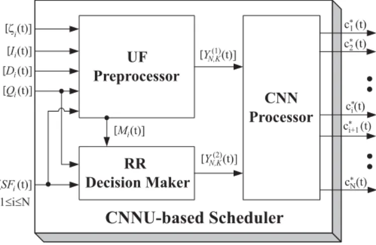
UF Preprocessor RR Decision Maker CNN Processor c (t)N* c (t)i+1* c (t)i* c (t)2* c (t)1* [Y (t)]N,K(2) [Y (t)]N,K(1) [M (t)]i [SF (t)]i [Q (t)]i [D (t)]i [I (t)]i [ζ (t)]i 1≤i≤ΝFig. 1. The block diagram of CNNU-based scheduler.
V. THECNNU-BASEDSCHEDULER
Figure 1 shows the block diagram of the CNN and utility (CNNU)-based scheduler. It contains a utility function (UF) preprocessor, a radio-resource range (RR) decision maker, and a CNN processor. The proposed CNNU-based scheduler takes the link information (𝜁𝑖(𝑡)), interference (ℐ𝑖(𝑡)), delay (𝐷𝑖(𝑡)), queue length (𝑄𝑖(𝑡)), and spreading factor (𝑆𝐹𝑖), 1 ≤ 𝑖 ≤ 𝑁, as inputs at the 𝑡-th frame, and finally outputs an optimal normalized radio resource (power) assignment vector
⇀𝑐∗(𝑡) = (𝑐∗
𝑖(𝑡), . . . , 𝑐∗𝑁(𝑡)), where 𝑐∗𝑖(𝑡), 1 ≤ 𝑖 ≤ 𝑁, is expressed by𝐾 bits. The quantization of the radio resource assignment vector into𝐾 bits is due to the nature of the binary expression of each neuron for the CNN processor. The higher the quantization level is, the higher the precision will be, but the more the convergence time of the CNN processor would be taken. Note that the ⇀𝑐∗(𝑡) can be for the current frame
or the next frame, depending on the convergence time of the CNN processor.
The UF preprocessor first calculates the utility function 𝒰𝑖(𝑡) given in (3), 1 ≤ 𝑖 ≤ 𝑁. Then it normalizes 𝒰𝑖(𝑡) by a compression function(1 − 𝑒−𝜎𝒰𝑖(𝑡)), expresses (1 − 𝑒−𝜎𝒰𝑖(𝑡))
to be an 1 × 𝐾 vector given by (15), and finally constructs an𝑁 × 𝐾 input matrix[𝑌𝑖,𝑘(1)]for the CNN processor, where 𝑌𝑖,𝑘(1) = (1 − 𝑒−𝜎𝒰𝑖(𝑡)) ⋅ 2−𝑘. Notice that the 𝜎 is a constant
related to the slope and the linear region of the compression function (1 − 𝑒−𝜎𝒰𝑖(𝑡)), which normalizes 𝑈𝑖(𝑡) ∈ [0, ∞)
into the range of[0, 1). A good compression function is the one with broad linear range so that the individual utility function is normalized linearly within a reasonable range. This normalization is to implement the first constraint in (14). The UF preprocessor also determines a vector of modula-tion order [𝑀𝜅𝑖] for all connections according to (8) and
outputs to the RR decision maker. The RR decision maker determines the upper limit for the radio resource assignment for every connection 𝑖 and expresses it by a 1 × 𝐾 vec-tor which is the upper limit multiplied by the bit-weighted vector (2−1, . . . , 2−𝑘, . . . , 2−𝐾), 1 ≤ 𝑖 ≤ 𝑁. Then the RR decision maker constructs the second input matrix [𝑌𝑖,𝑘(2)], 1 ≤ 𝑖 ≤ 𝑁, 1 ≤ 𝑘 ≤ 𝐾, where the element 𝑌𝑖,𝑘(2) is given by ( min{𝑊 ⋅log2𝑀𝜅𝑖 𝑆𝐹𝑖⋅ℛ𝑖(𝑡) , 𝑄𝑖(𝑡)/𝑇𝑓 ℛ𝑖(𝑡) })
⋅ 2−𝑘to implement the second
constraint in (14). The CNN processor receives the two input matrices,[𝑌𝑖,𝑘(1)]and[𝑌𝑖,𝑘(2)], and computes the optimal radio resource assignment vector ⇀𝑐∗(𝑡) for the 𝑡-th frame. During
the computation process, denote by 𝜏 the instantaneous time index of the CNN and by ⇀𝑐(𝑡, 𝜏) the instantaneous radio
resource assignment vector at time𝜏 during the frame 𝑡. For each𝑐𝑖(𝑡, 𝜏), 1 ≤ 𝑖 ≤ 𝑁, it is represented by K bits, 𝑋𝑖,𝑘(𝜏), 1 ≤ 𝑘 ≤ 𝐾, and 𝑐𝑖(𝑡, 𝜏) can be expressed by
𝑐𝑖(𝑡, 𝜏) ∼= 𝐾 ∑ 𝑘=1
𝑋𝑖,𝑘(𝜏) ⋅ 2−𝑘. (16)
When the CNN processor arrives at an equilibrium, the output will converge to the optimal radio resource assignment vector, ie., lim𝜏→∞⇀𝑐(𝑡, 𝜏) =⇀𝑐∗(𝑡).
In the following, the design of the CNN processor for the CNNU-based scheduler is described. Characteristics of the original CNN proposed in [13] are first briefed. Then, we define a cost function associated with the constrained opti-mization problem formulated in (14). Subsequently, we design an energy function based on the cost function. According to the trajectory of the energy function, we can construct the architecture of the desired CNN processor to fit the defined scheduling problem. Notice that it can be proven that the designed CNN processor can be with good stability and convergence [23], based on the principle of Lyapunov and the stability theorem of CNN [18], [19].
A. Preliminaries for Cellular Neural Networks
Consider a neural network with 𝑁 × 𝐾 neurons arranged in a rectangular array, where neuron (𝑖, 𝑘) is denoted by 𝑧𝑖,𝑘. The output of 𝑧𝑖,𝑘 at time 𝜏, denoted by 𝑋𝑖,𝑘(𝜏), can be expressed by 𝑋𝑖,𝑘(𝜏) = 𝑓(𝑋𝑖,𝑘(𝑠)(𝜏)), where 𝑓(𝑥) =
1
2[∣𝑥∣ − ∣𝑥 − 1∣] + 12 is an activation function of 𝑧𝑖,𝑘 and 𝑋𝑖,𝑘(𝑠)(𝜏) is the state variable of 𝑧𝑖,𝑘 at time 𝜏. The 𝑋𝑖,𝑘(𝑠)(𝜏) consists of recurrent inputs, external inputs, and a bias current. Each neuron 𝑧𝑖,𝑘 connects with all other neurons within its neighborhood, denoted by 𝑍𝑛(𝑖, 𝑘). The area of 𝑍𝑛(𝑖, 𝑘) is determined according to the design of the neural network. Generally, the dynamics of the CNN at time 𝜏 is represented by [13], [14], as (17), where𝜈 in (17) is a time constant for all neurons,𝐴𝑖,𝑘;𝑗,𝑚is the recurrent inter-connection weight from neuron𝑧𝑗,𝑚to𝑧𝑖,𝑘,𝐵𝑖,𝑘;𝑗,𝑚 is the control weight of external input from𝑧𝑗,𝑚to𝑧𝑖,𝑘,𝑌𝑗,𝑚is the external input to the neuron 𝑧𝑗,𝑚, and 𝑉𝑖,𝑘 is the bias current to 𝑧𝑖,𝑘, which is usually a fixed value 𝑉 . It is worth mentioning that 𝐴𝑖,𝑘;𝑖,𝑘 > 1/𝜈 is held so that the neuron 𝑧𝑖,𝑘 will eventually enter into a saturation region [13]. Also, the inter-connection weights are assumed to be symmetric, that is, 𝐴𝑖,𝑘;𝑗,𝑚 = 𝐴𝑗,𝑚;𝑖,𝑘, thus the CNN is stable [13].
An energy function at time 𝜏 which decreases along the trajectories of (17), denoted by ℰ(𝜏), is generally expressed by [13], as (18). At the stable state, outputs of neurons will arrive at an equilibrium with the minimum energy function. If the energy function is properly designed and acts as a cost function, such an optimization problem can be solved via the Lyapunov method [15]-[19]. By the Lyapunov method, the CNN can be designed with a set of prescribed trajectories.
( (1 − 𝑒−𝜎𝒰𝑖(𝑡)) ⋅ 2−1, . . . , (1 − 𝑒−𝜎𝒰𝑖(𝑡)) ⋅ 2−𝑘, . . . , (1 − 𝑒−𝜎𝒰𝑖(𝑡)) ⋅ 2−𝐾) (15) 𝑑𝑋𝑖,𝑘(𝑠)(𝜏) 𝑑𝜏 = − 𝑋𝑖,𝑘(𝑠)(𝜏) 𝜈 + 𝐴𝑖,𝑘;𝑖,𝑘⋅ 𝑋𝑖,𝑘(𝜏) + 𝐵𝑖,𝑘;𝑖,𝑘⋅ 𝑌𝑖,𝑘 + ∑ 𝑧𝑗,𝑚∈𝑍𝑛(𝑖,𝑘) 𝐴𝑖,𝑘;𝑗,𝑚⋅ 𝑋𝑗,𝑚(𝜏) + ∑ 𝑧𝑗,𝑚∈𝑍𝑛(𝑖,𝑘) 𝐵𝑖,𝑘;𝑗,𝑚⋅ 𝑌𝑗,𝑚+ 𝑉𝑖,𝑘 (17) ℰ(𝜏) = −12 𝑁 ∑ 𝑖=1 𝐾 ∑ 𝑘=1 𝐴𝑖,𝑘;𝑖,𝑘𝑋2 𝑖,𝑘(𝜏) −12 𝑁 ∑ 𝑖=1 𝐾 ∑ 𝑘=1 𝑁 ∑ 𝑗=1 𝐾 ∑ 𝑚=1 𝐴𝑖,𝑘;𝑗,𝑚𝑋𝑗,𝑚(𝜏)𝑋𝑖,𝑘(𝜏) −12 𝑁 ∑ 𝑖=1 𝐾 ∑ 𝑘=1 𝑁 ∑ 𝑗=1 𝐾 ∑ 𝑚=1 𝐵𝑖,𝑘;𝑗,𝑚𝑌𝑗,𝑚𝑋𝑖,𝑘(𝜏) − 𝑁 ∑ 𝑖=1 𝐾 ∑ 𝑘=1 𝑉𝑖,𝑘⋅ 𝑋𝑖,𝑘(𝜏) (18)
The trajectories are described by the gradient of the Lyapunov functionℰ(𝜏) which is the energy of the CNN network at time 𝜏. With an appropriate energy function designed according to the cost function, the minimization of the cost can be achieved along the designed trajectories. In the mean time, it can be proved that the architecture of the designed CNN can be related with the energy function by
𝑑𝑋𝑖,𝑘(𝑠)(𝜏) 𝑑𝜏 = − 𝑋𝑖,𝑘(𝑠)(𝜏) 𝜈 − ∂ℰ(𝜏) ∂𝑋𝑖,𝑘(𝜏). (19) Using (19), the desired system parameters of inter-connection weights, control weights, and bias currents can be found from the trajectories of energy function.
B. Cost Function of CNN Processor
The cost function of the proposed CNN processor to achieve the optimal resource allocation at time 𝜏 during frame 𝑡, denoted byℋ(𝑡, 𝜏), consists of a cost function for the utility function, denoted byℋ𝑢(𝑡, 𝜏), in conjunction with cost func-tions for system constraintsΨ1andΨ2given in (14), denoted
byℋΨ1(𝑡, 𝜏) and ℋΨ2(𝑡, 𝜏), respectively. The ℋ(𝑡, 𝜏) has the
form of
ℋ(𝑡, 𝜏) = ℋ𝑢(𝑡, 𝜏) + ℋΨ1(𝑡, 𝜏) + ℋΨ2(𝑡, 𝜏). (20)
The ℋ𝑢(𝑡, 𝜏) is defined to be the difference between an overall normalized utility function and its maximum, where the overall normalized utility function is defined as ∑𝑁
𝑖=1𝑐𝑖(𝑡, 𝜏)⋅ (1 − 𝑒−𝜎𝒰𝑖(𝑡)). When ∑𝑁
𝑖=1𝑐𝑖(𝑡, 𝜏) ≤ 1, ∑𝑁
𝑖=1𝑐𝑖(𝑡, 𝜏) ⋅ (1 − 𝑒−𝜎𝒰𝑖(𝑡)) is bounded by 1. Thus the ℋ𝑢(𝑡, 𝜏) is given by ℋ𝑢(𝑡, 𝜏) = 𝜂0 [ 1 − 𝑁 ∑ 𝑖=1 𝑐𝑖(𝑡, 𝜏)(1 − 𝑒−𝜎𝒰𝑖(𝑡))], (21)
where𝜂0 is the coefficient ofℋ𝑢(𝑡, 𝜏).
The ℋΨ1(𝑡, 𝜏) is defined as ℋΨ1(𝑡, 𝜏) = 𝜂1 [𝑁 ∑ 𝑖=1 𝑐𝑖(𝑡, 𝜏) − 1 ]2 , (22) where 𝜂1 = 𝜂1+ ⋅ 𝑢(∑𝑁𝑖=1𝑐𝑖(𝑡, 𝜏) − 1 ) + 𝜂− 1 ⋅ ( 1 − 𝑢(∑𝑁𝑖=1𝑐𝑖(𝑡, 𝜏) − 1 ))
, 𝑢(⋅) is the unit-step function, 𝜂+
1 is the slope constant for the cost increment when the total
radio resource is greater than the maximum, and 𝜂− 1 is the
slope constant for the cost increment otherwise. The ranges of 𝜂+
1 and𝜂−1 are further investigated in the next section to
ensure the stability and the desired output pattern of the CNN processor.
The ℋΨ2(𝑡, 𝜏) is defined to be proportional to the
differ-ence[𝑐𝑖(𝑡, 𝜏) − min{𝑊 ⋅log2𝑀𝜅𝑖
𝑆𝐹𝑖⋅ℛ𝑖(𝑡) , 𝑄𝑖(𝑡)/𝑇𝑓 ℛ𝑖(𝑡) }] if 𝑐𝑖(𝑡, 𝜏) > min{𝑊 ⋅log2𝑀𝜅𝑖 𝑆𝐹𝑖⋅ℛ𝑖(𝑡) , 𝑄𝑖(𝑡)/𝑇𝑓 ℛ𝑖(𝑡) }
; otherwise, no cost will be in-curred because the radio resource will be allocated to other connections for efficiency. It is given by (23), where𝜂2is the
coefficient of ℋΨ2(𝑡, 𝜏); (𝑎)+ = 𝑎 if 𝑎 ≥ 0, (𝑎)+ = 0 if
𝑎 < 0.
C. The Architecture of CNN Processor
According to the cost functionℋ(𝑡, 𝜏) at time 𝑡, the energy function ℰ(𝑡, 𝜏) can be designed for the CNN processor in the CNNU-based scheduler. However, some modifications on ℋ(𝑡, 𝜏) in (20) should be made for ℰ(𝑡, 𝜏) to ensure the correctness of the desired output and the stability of the CNN processor. Theℰ(𝑡, 𝜏) is given by (24), where 𝜂3is a constant
for additional auxiliary terms. The first three terms of (24) are convex function for the ℰ(𝑡, 𝜏), which are transformed from the three concave functions of theℋ(𝑡, 𝜏), respectively. However, several constants are removed to simplify the ar-chitecture of CNN with the equilibrium unchanged. The first item differs from (21) in that the scalar 1 is ignored and the remaining term ∑𝑁𝑖=1(∑𝐾𝑘=1𝑋𝑖,𝑘(𝜏) ⋅ 2−𝑘) ⋅ (1 − 𝑒−𝜎⋅𝒰𝑖(𝑡))
is bounded above by 1 and has the same minimum as in the cost function. For the second and the third terms, the quadratic forms in (22) and (23) are replaced by convex functions which merely contain state variable𝑋𝑖,𝑘(𝜏) without any scalar. The local minimums would be the same; the resulting energy at any equilibrium would be shifted by a constant value, compared to the cost in (20), and independent of the inputs and the output pattern. The last term of (24) is an auxiliary factor to ensure the convergence of the whole CNN to one of its vertex.
2-K 2-k 2-1 2-1 2-k 2-K
Decision Layer
Output Layer
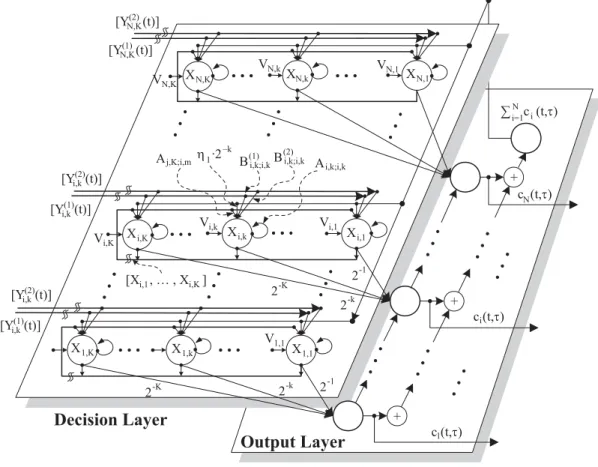
[X , … , X ]i,1 i,K N i=1 i Ai,k;i,k B(2)i,k;i,k Bi,k;i,k(1) Aj,K;i,m η ·21 –k [Y (t)]i,k(1) [Y (t)]i,k(2) [Y (t)]i,k(1) [Y (t)]i,k(2) XN,1 VN,1 VN,K VN,k XN,k XN,K Vi,1 X i,1 V1,1 X 1,1 Vi,k X i,k X1,k Vi,K Xi,K X1,K [Y (t)]N,K(1) [Y (t)]N,K(2) + + + ∑ c (t,τ) N c (t,τ) i c (t,τ) 1 c (t,τ)Fig. 2. The two-layer structure of CNN processor.
ℋΨ2(𝑡, 𝜏) = 𝜂2 ⎡ ⎣∑𝑁 𝑖=1 (( 𝑐𝑖(𝑡, 𝜏) − min { 𝑊 ⋅ log2𝑀𝜅𝑖 𝑆𝐹𝑖⋅ ℛ𝑖(𝑡) , 𝑄𝑖(𝑡)/𝑇𝑓 ℛ𝑖(𝑡) })+)2⎤ ⎦ (23)
The necessity of this auxiliary term is shown in Lemma 2 in [23]. When the coefficient 𝜂3 is properly selected as shown
in Lemma 6 in [23], the energy function due to this auxiliary term will approach zero only when every state variable output approaches either one or zero, which is one of the CNN vertex. By (19) and (24), the dynamics of each neuron in the proposed CNN processor for the CNNU-based scheduler can be expressed by (25), where 𝜈𝑘 is modified to 2𝑘 to retain the stability and desired output pattern of the designed CNN processor. From (17) and (25), we can determine the inter-connection structure of the CNN processor. The complexity of the CNN has an order of𝑂(𝑁2).
In order to reduce the complexity of CNN processor, we propose a two-layer structure for the CNN processor, which the complexity has an order of 𝑂(𝑁𝐾). Note that the 𝐾 is bounded by the precision and 𝐾 ≪ 𝑁. To re-arrange (25) and replace ∑𝐾𝑘=1𝑋𝑖,𝑘(𝑡) by 𝑐𝑖(𝑡, 𝜏) and in contrast to (17), the first decision layer,[𝑧1
𝑖,𝑘 ]
, is with state variable output 𝑋𝑖,𝑘(𝜏), which is determined by regarding the term of 𝑐𝑖(𝑡, 𝜏) as a constant. The second output layer,
[ 𝑧2
𝑖,𝑘 ]
, is with state variable output 𝑐𝑖(𝑡, 𝜏), which is determined by regarding the term of ∑𝐾𝑘=1𝑋𝑖,𝑘(𝑡) as a constant. The decision layer consists of𝑁 × 𝐾 neurons; the output layer is
with an(𝑁+1)×1 array, where the output of the first neuron is the summation of all the others. The inter-connections between the neurons of decision layer and those of output layer are defined by
∙ For the first decision layer to the second output layer, the connection weight between𝑋𝑖,𝑘(𝜏) and 𝑐𝑗(𝑡, 𝜏) is 2−𝑘,∀𝑘 if 𝑗 = 𝑖; zero if 𝑗 ∕= 𝑖.
∙ For the second output layer feedback to the first decision layer, only the first neuron output is connected to the 𝑋𝑖,𝑘(𝜏) of the decision layer with the inter-connection weight𝜂1⋅ 2−𝑘 for∀𝑖.
Fig. 2 shows the two-layer structure of the CNN processor. The recurrent inter-connection weights and the external control weights for the first decision layer can be determined by (26), where 𝐵𝑖,𝑘;𝑖;𝑘(1) and 𝐵𝑖,𝑘;𝑖;𝑘(2) are the external control weights for the first and the second external inputs, 𝑌𝑖,𝑘(1) = ( 1 − 𝑒−𝜎𝒰𝑖(𝑡))⋅2−𝑘and𝑌(2) 𝑖,𝑘 = min { 𝑊 ⋅log2𝑀𝜅𝑖 𝑆𝐹𝑖⋅ℛ𝑖(𝑡) , 𝑄𝑖(𝑡)/𝑇𝑓 ℛ𝑖(𝑡) } ⋅ 2−𝑘, respectively, and 𝛿 𝑥,𝑦= 1 if 𝑥 = 𝑦; 𝛿𝑥,𝑦 = 0 otherwise. For the second output layer, there are no external inputs, and only the recurrent connection weights exist. The inter-connection weight between 𝑐𝑖(𝑡, 𝜏) and 𝑐𝑗(𝑡, 𝜏) is given by 𝛿0,𝑗 with𝑖 = 0.
ℰ(𝑡, 𝜏) = −𝜂0 [ 𝑁 ∑ 𝑖=1 (∑𝐾 𝑘=1 𝑋𝑖,𝑘(𝜏) ⋅ 2−𝑘) ⋅ (1 − 𝑒−𝜎⋅𝒰𝑖(𝑡)) ] +𝜂1 [( 𝑁 ∑ 𝑖=1 1 2( 𝐾 ∑ 𝑘=1 𝑋𝑖,𝑘(𝜏) ⋅ 2−𝑘) − 1 ) ⋅ ( 𝑁 ∑ 𝑖=1 (∑𝐾 𝑘=1 𝑋𝑖,𝑘(𝜏) ⋅ 2−𝑘) )] +𝜂2 ⎡ ⎣∑𝑁 𝑖=1 ⎛ ⎝ ( 1 2( 𝐾 ∑ 𝑘=1 𝑋𝑖,𝑘(𝜏) ⋅ 2−𝑘) − min { 𝑊 ⋅ log2𝑀𝜅𝑖 𝑆𝐹𝑖⋅ ℛ𝑖(𝑡) , 𝑄𝑖(𝑡)/𝑇𝑓 ℛ𝑖(𝑡) })+ ⋅ ( 𝐾 ∑ 𝑘=1 𝑋𝑖,𝑘(𝜏) ⋅ 2−𝑘) )] + 𝜂3 [𝑁 ∑ 𝑖=1 (𝐾 ∑ 𝑘=1 𝑋𝑖,𝑘(𝜏)(1 − 𝑋𝑖,𝑘(𝜏))⋅ 2−𝑘 )] (24) 𝑑𝑋𝑖,𝑘(𝑠)(𝜏) 𝑑𝜏 = − 𝑋𝑖,𝑘(𝑠)(𝜏) 𝜈𝑘 + 𝜂0 ( 1 − 𝑒−𝜎𝒰𝑖(𝑡))⋅ 2−𝑘− 𝜂 1 (𝑁 ∑ 𝑖=1 𝐾 ∑ 𝑘=1 𝑋𝑖,𝑘(𝜏) ⋅ 2−𝑘− 1 ) ⋅ 2−𝑘 −𝜂2 ( 𝐾 ∑ 𝑚=1 𝑋𝑖,𝑚(𝜏) ⋅ 2−𝑚− min{𝑊 ⋅ log2𝑀𝜅𝑖 𝑆𝐹𝑖⋅ ℛ𝑖(𝑡) , 𝑄𝑖(𝑡)/𝑇𝑓 ℛ𝑖(𝑡) })+ ⋅ 2−𝑘 −𝜂3(1 − 2𝑋𝑖,𝑘(𝜏)) ⋅ 2−𝑘 = −𝑋 (𝑠) 𝑖,𝑘(𝜏) 𝜈𝑘 + [ 2𝜂3⋅ 2−𝑘− 𝜂1⋅ 2−2𝑘− 𝜂2⋅ 𝑢 (𝐾 ∑ 𝑘=1 𝑋𝑖,𝑘− min { 𝑊 ⋅ log2𝑀𝜅𝑖 𝑆𝐹𝑖⋅ ℛ𝑖(𝑡) , 𝑄𝑖(𝑡)/𝑇𝑓 ℛ𝑖(𝑡) }) ⋅ 2−2𝑘]⋅ 𝑋𝑖,𝑘(𝜏) + 𝜂 0 ( 1 − 𝑒−𝜎𝒰𝑖(𝑡))⋅ 2−𝑘 +𝜂2⋅ 𝑢 ( 𝐾 ∑ 𝑚=1 𝑋𝑖,𝑚(𝜏) ⋅ 2−𝑚− min{𝑊 ⋅ log2𝑀𝜅𝑖 𝑆𝐹𝑖⋅ ℛ𝑖(𝑡) , 𝑄𝑖(𝑡)/𝑇𝑓 ℛ𝑖(𝑡) }) ⋅ min { 𝑊 ⋅ log2𝑀𝜅𝑖 𝑆𝐹𝑖⋅ ℛ𝑖(𝑡) , 𝑄𝑖(𝑡)/𝑇𝑓 ℛ𝑖(𝑡) } ⋅ 2−𝑘− ⎛ ⎝ ∑𝑁 𝑗=1,𝑗∕=𝑖 𝐾 ∑ 𝑚=1 𝜂1⋅ 2−(𝑚+𝑘)⋅ 𝑋𝑗,𝑚(𝜏) ⎞ ⎠ − ⎛ ⎝ ∑𝐾 𝑚=1,𝑚∕=𝑘 [ 𝜂1− 𝜂2⋅ 𝑢 ( 𝐾 ∑ 𝑚=1 𝑋𝑖,𝑚(𝜏) ⋅ 2−𝑚− min { 𝑊 ⋅ log2𝑀𝜅𝑖 𝑆𝐹𝑖⋅ ℛ𝑖(𝑡) , 𝑄𝑖(𝑡)/𝑇𝑓 ℛ𝑖(𝑡) })] ⋅ 2−(𝑚+𝑘)⋅ 𝑋 𝑖,𝑚(𝜏) ) + 𝜂1⋅ 2−𝑘− 𝜂3⋅ 2−𝑘 (25) ⎧ ⎨ ⎩ 𝐴𝑖,𝑘;𝑖;𝑘= −𝜂1⋅ 2−2𝑘− 𝜂2⋅ 𝑢(∑𝐾𝑘=1𝑋𝑖,𝑘− min { 𝑊 ⋅log2𝑀𝜅𝑖 𝑆𝐹𝑖⋅ℛ𝑖(𝑡) , 𝑄𝑖(𝑡)/𝑇𝑓 ℛ𝑖(𝑡) }) ⋅ 2−2𝑘+ 2𝜂3, 𝐵𝑖,𝑘;𝑖;𝑘(1) = 𝜂0, 𝐵𝑖,𝑘;𝑖;𝑘(2) = 𝜂2⋅ 𝑢(∑𝐾𝑘=1𝑋𝑖,𝑘− min { 𝑊 ⋅log2𝑀𝜅𝑖 𝑆𝐹𝑖⋅ℛ𝑖(𝑡) , 𝑄𝑖(𝑡)/𝑇𝑓 ℛ𝑖(𝑡) }) , 𝐴𝑖,𝑘;𝑗;𝑚= −𝜂2⋅ 𝑢(∑𝐾𝑘=1𝑋𝑖,𝑘− min { 𝑊 ⋅log2𝑀𝜅𝑖 𝑆𝐹𝑖⋅ℛ𝑖(𝑡) , 𝑄𝑖(𝑡)/𝑇𝑓 ℛ𝑖(𝑡) }) ⋅ 𝛿𝑖,𝑗⋅ 2−(𝑘+𝑚), 𝑉𝑖,𝑘 = 𝜂1⋅ 2−𝑘− 𝜂3. (26)
be properly selected to ensure the stability and the desired response. For a tolerant error level𝜀, which is the maximum difference between stable output lim𝜏→∞⇀𝑐(𝑡, 𝜏) and the optimum⇀𝑐∗(𝑡), the ranges of these coefficients are obtained
as follows [23]: 0 < 𝜂0 < 𝜂3 , 𝜂1+ > 2𝐾, 𝜂−1 ≥ 𝜂0⋅2 −3 𝜀 , 𝜂2 ≥ 2𝐾,𝜂3> 12+𝜂 − 1
2 . We have proved in [23] that with a
matrix of given utility function and a matrix of radio resource assignment ratio upper limits, the proposed architecture of CNN processor will converge to the neighborhood of the optimal pattern⇀𝑐∗(𝑡) within the difference 𝜀, with the ranges
of these coefficients. If 𝜀 ≤ 2−𝐾, the CNN can converge to
⇀𝑐∗(𝑡). Note that the complexity of inter-connections in the
two-layer CNN processor is proportional to [3𝑁 × 𝐾 + 𝑁], which is linear with respect to the number.
VI. SIMULATIONRESULTS ANDDISCUSSION
In simulations, a scenario with five types of services in three classes is assumed. Type-1 service is a real-time class of traffic with a peak rate of 15 kbps, an activity factor of 0.57,𝑃∗
𝐷 = 0.05, 𝐷∗ = 40 ms, and 𝐵𝐸𝑅∗ = 10−3; type-2 (type-3) service is a non-real-time interactive class of traffic with Pareto process [24] of which the mean rate is 8 kbps (12 kbps), 𝑅∗
𝑚,𝑖=7.2 kbps (𝑅∗𝑚,𝑖=11 kbps), and 𝐵𝐸𝑅∗ = 10−5 (𝐵𝐸𝑅∗ = 10−5); and type-4 (type-5) service is a non-real-time best effort class of traffic in batch Poisson distribution with a mean rate of 6 kbps (15 kbps) and a mean batch size of 1.2 kbits (1.2 kbits), and𝐵𝐸𝑅∗ = 10−5. The proportion in the number of connections from type-1 to type-5 is kept at 1:1:1:1:1. Also, three modulation schemes, QPSK, 16QAM, and 64QAM, are available for transmission as long as the BER requirement can be fulfilled and the remaining queue is enough.
We compare the proposed CNNU-based radio resource scheduler with the EXP scheduling scheme [9] and the HOLPRO scheme [5]. The EXP scheduling scheme can be directly extended for RT and NRT connections. However, the HOLPRO scheme is only suitable for RT connections. As for NRT connections, the pseudoprobability is obtained according to the fraction between the queue length of the connection and the summed queue length among all NRT connections. Also, the RT connections have absolutely higher priority than the NRT connections.
The performance measures are such as the average system throughput, the average packet dropping ratio of RT connec-tions, 𝑃𝐷, the average transmission rate of NRT interactive connections,𝑅𝑚, the ratio of RT connections in which their packet dropping ratio requirement is not guaranteed,𝜙𝑃𝐷, the
ratio of NRT interactive connections in which their minimum transmission rate requirement is not guaranteed,𝜙𝑅𝑚, and the
fairness variance index of NRT connections,𝐹𝑣.
The 𝐹𝑣 is defined for measuring the variance of fairness to share the radio resource among all NRT connections. It is given by 𝐹𝑣= 𝑁1 𝑁𝑅𝑇 𝑁∑𝑁𝑅𝑇 𝑖 (( (( ((∑𝑁𝑁𝑅𝑇E [𝑟𝑖(𝑡)] 𝑗 E [𝑟𝑗(𝑡)] −∑𝑁𝑤𝑖 𝑁𝑅𝑇 𝑗 𝑤𝑗 (( (( (( 2 , (27) where𝑁𝑁𝑅𝑇 is the number of NRT connections. The fairness
variance index shows the variance of the normalized radio
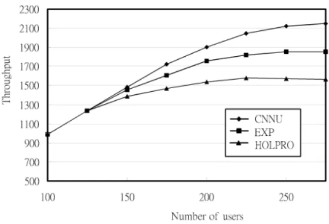
Fig. 3. The average system throughput.
resource allocated and the normalized proportion of resource desired to share.
At first, we measure the stability and the convergence of the CNN processor during the simulation. The measure of stability of the CNN processor is assumed to be the percentage of which the output of each neuron 𝑧1
𝑖,𝑘 takes the value from {0, 1} and no chaotic state occurs; the measure of convergence of the CNN processor is assumed to be the percentage of which the output of neurons𝑧2
𝑖,𝑘 is within the system constraints Ψ1 and Ψ2. It is found that the CNN
processor can always be stable without chaotic trajectory. Also, the output ⃗𝑐𝑖(𝑡) can mostly converge to a reasonable set of stable output of the CNN processor in a percentage of about 99.9%. On the other hand, the convergence speed of CNN processor would be in few miniseconds range [15], [18] since the CNN has an architecture that all neurons are in the same structure, which makes the CNN be suitable for VLSI implementation.
Fig. 3 shows the average system throughput. It can be found that the CNNU-based scheduler can always have a higher sys-tem capacity than the EXP and HOLPRO scheduling schemes in all traffic load conditions. It achieves the improvement of system throughput over the EXP (HOLPRO) scheduling scheme by more than 9% (19%) as the number of connections is greater than 200, and by higher than 15% (25%) as the number of connections increases up to 250. This is because the CNNU-based scheduler is with the radio resource function that makes CNN processor adapt to the link variation and allocate radio resource in an efficient way. Both RT and NRT connections with relatively worse link conditions have lower probability to be scheduled as long as their QoS requirements can be achieved in a long term sense. The CNNU-based scheduler is with the fairness compensation function that makes the NRT connections share the radio resource according to the location dependent fairness, achieving a higher radio resource efficiency. Also, the CNN processor can determine an optimal radio resource assignment vector in the sense that the allocation of downlink power by CNNU-based scheduler is the most efficient one, with given utilities and upper limits of the radio resource assignment. Additionally, beyond the point of 250 (200) connections, the throughput of the EXP
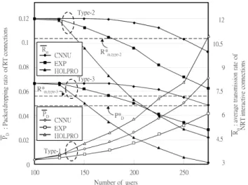
Fig. 4. QoS performance measures of packet dropping ratio𝑃𝐷and average
transmission rate𝑅𝑚.
(HOLPRO) scheme is almost saturated, while the throughput of the CNNU-based scheduler continues to grow up but with a slightly lowering slope. It is because the CNNU-based scheduler can achieve the utilization of multiuser diversity gain better than the EXP scheduling scheme. The HOLPRO scheme always has the lowest throughput among these three schemes due to the lack of link condition information.
Fig. 4 depicts the performance measures of the average packet dropping ratio of type-1 RT connections𝑃𝐷 and the average transmission rate of type-2 and type-3 NRT interaction connections𝑅𝑚. It can be found that the𝑃𝐷 of the CNNU-based scheduler is larger than that of the EXP scheme but lower than that of HOLPRO scheme, and it violates the𝑃∗
𝐷 requirement as the number of users is about 250; on the other hand, all the 𝑅𝑚 of type-2 and type-3 connections of the CNNU-based scheduler are greater than those of the EXP and HOLPRO schemes, and the EXP (HOLPRO) scheme violates the 𝑅∗
𝑚 requirements as the number of users is about 170 (150). These indicate that the QoS guaranteed region by the CNNU-based scheduler can be up to 250 connections, while those by the EXP and HOLPRO schemes are only to 175 and 150 connections, respectively. The QoS guaranteed region achieved by the CNNU-based scheduler is larger than those achieved by the EXP and HOLPRO schemes. This is because the CNNU-based scheduler is designed with the QoS deviation function together with the priority bias that can balance the extent of deviation of every performance measure from the QoS requirement. The worse the QoS performance measure is, the more the radio resource will be scheduled. Besides, since the CNNU-based scheduler has higher throughput per-formance, the more number of connections can be served in the QoS guaranteed region. Moreover, if we define the maximum throughput achievable in QoS guaranteed region to be the average system throughput, the CNNU-based scheduler can have the average system throughput equal to 2.083 Mbps at 235 connections, while the EXP and the HOLPRO schemes can have the average system throughput equal to 1.6 Mbps at 175 connections and 1.388 Mbps at 150 connections,
Fig. 5. The ratio 𝜙𝑃𝐷 for RT connections and the ratio𝜙𝑅𝑚 for NRT
interactive connections.
respectively. The former attains the average system throughput greater than the latter by an amount of 23% and 33%, respectively.
Fig. 5 shows the ratio of RT connections of which the packet dropping ratio requirement is not guaranteed, 𝜙𝑃𝐷, and the
ratio of NRT interactive connections of which the minimum transmission rate requirement is not guaranteed,𝜙𝑅𝑚. It can be
seen that the total ratio of connections with QoS requirements un-guaranteed for the CNNU-based scheduler is about 0.0435, while those for the EXP and HOLPRO schemes are greater than 0.18 and 0.365, respectively, in heavily loaded situations as the number of connections is greater than 225. The total ratio of connections with QoS requirements un-guaranteed is defined as 1
3𝜙𝑃𝐷 +23𝜙𝑅𝑀, which is weighted by the number
of RT and NRT interactive connections.
The CNNU-based scheduler can achieve the total ratio of QoS requirements un-guaranteed connections in all traffic types lower than the EXP and HOLPRO scheme. The reason is that the CNNU-based scheduler can balance the allocation of radio resources among traffic types and avoid allocating excess radio resource to connections with bad link condition, while the EXP and HOLPRO schemes prefer RT connections and overprotects them so that the QoS guaranteed region is reduced. Note that the ratios of 𝜙𝑃𝐷 and 𝜙𝑅𝑚 are greater
than zero at any traffic load condition due to the existence of connections with very bad link quality. These results imply that the CNNU-based scheduler will not guarantee all the QoS requirements all the time, and a properly designed call admission control is required to reject the connections with very bad link quality in terms of the current traffic load conditions.
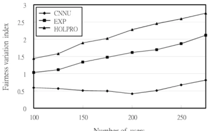
Fig. 6 shows the fairness variance index of NRT connec-tions. It can be found that the fairness variance indexes of the CNNU-based scheduler retains within 1 in almost all simulation cases, and grows up slowly as the number of connections increases; the fairness variance indexes of the EXP and HOLPRO schemes, on the other hand, increase with slightly higher slope than that of the CNNU-based sched-uler. This is because the fairness compensation function of the CNNU-based scheduler considers the location dependent information and aims to share the radio resource fairly as long as the minimum rate is guaranteed, while the design
Fig. 6. The fairness variation index for NRT connections.
of the EXP and the HOLPRO schemes ignore the location dependent information to allocate rate fairly to all connections. The fairness compensation function, considering the location dependent information, also facilitates the higher capacity for the CNNU-based scheduler shown in Fig. 3.
VII. CONCLUDINGREMARKS
This paper presents a cellular neural network and utility (CNNU)-based radio resource scheduler, which jointly con-siders its radio resource efficiency, diverse QoS requirements, and fairness, to schedule the radio resource for downlink connections in multimedia CDMA communication systems. The utility function is defined to be the radio resource function properly weighted by the QoS requirement deviation function and the fairness compensation function. Also, the cellular neural network (CNN) is successfully manipulated to be a two-layer structure to solve the constrained optimization problem defined for the radio resource scheduling in a real-time fashion. Simulation results show that the CNNU-based scheduler can efficiently allocate the radio resource to achieve higher throughput than the conventional EXP and HOLPRO scheduling schemes. It can also effectively support differen-tiated QoS requirements for connections with various traffic characteristics. Moreover, the CNNU-based scheduler can enlarge the QoS guaranteed region under the complicated QoS requirements. The CNNU-based radio resource scheduler is effective for multimedia CDMA communciation systems with diverse QoS requirements when both dedicated and shared channels are adopted.
ACKNOWLEDGMENT
The authors would like to give many thanks to those anonymous reviewers for their kind helps to improve the presentation of the paper.
REFERENCES
[1] 3rd Generation Partnership Project (June 2001), QoS Concept and Architecture, 3GPP TS 23.107. Online: http://www.3gpp.org. [2] Y. M. Lu and R. W. Brodersen, “Integrating power control, error
correction coding, and scheduling for a CDMA downlink system,” IEEE
J. Select. Areas Commun., vol. 17, no. 5, pp. 978-989, May 1999.
[3] V. K. N. Lau and Y. K. Kwok, “On generalized optimal scheduling of high data-rate bursts in CDMA systems,” IEEE Trans. Commun., vol. 51, no. 2, pp. 261-266, Feb. 2003.
[4] V. Bharghavan, S. W. Lu, and T. Nandagopal, “Fair queuing in wireless networks: issues and approaches,” IEEE Personal Commun., vol. 6, no. 1, pp. 44-53, Feb. 1999.
[5] A. C. Varsou and H. V. Poor, “HOLPRO: a new rate scheduling algorithm for the downlink of CDMA networks,” in Proc. IEEE VTC
2000, pp. 948-954.
[6] ——–, “Waiting time analysis for the generalized PEDF and HOLPRO algorithms in a system with heterogeneous traffic,” in Proc. IEEE VTC
2001, pp. 2152-2156.
[7] A. L. Stolyar and K. Ramanan, “Largest weighted delay first scheduling: large deviations and optimality,” Annal Appl. Prob., vol. 11, no. 1, pp. 1-48, 2001.
[8] A. C. Kam, T. Minn, and K. Y. Siu, “Supporting rate guarantee and fair access for bursty data traffic in W-CDMA,” IEEE J. Select. Areas
Commun., vol. 19, no. 11, pp. 2121-2130, 2001.
[9] S. Shakkottai and A. L. Stolyar, “Scheduling algorithms for a mixture of real-time and non-real-time data in HDR,” Bell Lab Reports, 2000. [10] C. X. Li, X. D. Wang, and D. Reynolds, “Rate control and fairness
scheduling for downlink utility-based power control systems,” in Proc.
IEEE GLOBECOM 2004, pp. 465-469.
[11] S. Haykin, Neural Networks: A Comprehensive Foundation. New York: MacMillan, 1994.
[12] S. Abe, “Global convergence and suppression of spurious states of Hopfield neural networks,” IEEE Trans. Circuits Syst., vol. 40, no. 4, pp. 246-257, 1993.
[13] L. O. Chua and L. Yang, “Cellular neural networks: theory,” IEEE Trans.
Circuits Syst., vol. 35, no. 10, pp. 1257-1272, Oct. 1988.
[14] “Cellular neural networks: applications,” IEEE Trans. Circuits Syst., vol. 35, no. 10, pp. 1273-1290, Oct. 1988.
[15] J. A. Nossek, “Design and learning with cellular neural networks,” in
Proc. IEEE CNNA-1994, Rome, pp. 137-146, Dec. 1994.
[16] R. Fantacci, M. Forti, M. Marini, and L. Pancani, “Cellular neural network approach to a class of communication problems,” IEEE Trans.
Circuits Syst., vol. 46, no. 12, pp. 1457-1467, Dec. 1999.
[17] S. Shen and C. J. Chang, “A cellular neural network and utility-based scheduler for multimedia CDMA cellular networks,” in Proc. IEEE
IWCMC 2005, pp. 768-773.
[18] W. E. Lillo, M. H. Loh, S. Hui, and S. H. Zak, “On sovling con-strained optimization problems with neural networks: a penalty method approach,” IEEE Trans. Neural Net., vol. 4, no. 6, pp. 931-940, Nov. 1993.
[19] C. C. Chiu, C. Y. Maa, and M. A. Shanblatt, “Energy function analysis of dynamic programming neural networks,” IEEE Trans. Neural Net., vol. 2, no. 4, pp. 418-426, July 1991.
[20] A. J. Goldsmith and S. G. Chua, “Variable-rate variable-power MQAM for fading channels,” IEEE Trans. Commun., vol. 45, no. 10, pp. 1218-1230, Oct. 1997.
[21] M. Andrews, K. Kumaran, K. Ramanan, A. Stolyar, P. Whiting, and R. Vijayakumar, “Providing quality of service over a shared wireless link,”
IEEE Commun. Mag., vol. 39, no. 2, pp. 150-154, Feb. 2001.
[22] C. S. Chang and J. A. Thomas, “Effective bandwidth in high-speed digital networks,” IEEE J. Select. Areas Commun., vol. 13, no. 6, pp. 1091-1100, Aug. 1995.
[23] S. Shen, “The connection admission control and radio resource al-locations for multimedia WCDMA Networks,” doctoral dissertation, National Chiao Tung University, 2005.
[24] Universal Mobile Telecommunications System (UMTS), Selection pro-cedures for the choice of radio transmission technologies of the UMTS, UMTS 30.03, version 3.2.0, 1998.
Scott Shen (S’99) received the B.S. degree in
electronics engineering from National Tsing Hua University, Hsing-Chu, Taiwain, in 1996, the M.A. and Ph.D degree in communication engineering from National Chiao Tung University, Hsing-Chu, Taiwain, in 1998 and 2005. His interest area includes wireless networks, mobile communications, high-speed networks, communications protocol design, and network performance evaluation. He is currently focusing the research areas on resource management for cellular networks.
Chung-Ju Chang was born in Taiwan, ROC, in
August 1950. He received the B.E. and M.E. degrees in electronics engineering from National Chiao Tung University, Hsinchu, Taiwan, in 1972 and 1976, respectively, and the Ph. D degree in electrical engineering from National Taiwan University, Tai-wan, in 1985. From 1976 to 1988, he was with Telecommunication Laboratories, Directorate Gen-eral of Telecommunications, Ministry of Communi-cations, Taiwan, as a Design Engineer, Supervisor, Project Manager, and then Division Director. He also acted as a Science and Technical Advisor for the Minister of the Ministry of Communications from 1987 to 1989. In 1988, he joined the Faculty of the Department of Electrical Engineering, College of Electrical and Computer Engineering, National Chiao Tung University, as an Associate Professor. He has been a Professor since 1993. He was Director of the Institute of Communication Engineering from August 1993 to July 1995, Chairman of Department of Communication Engineering from August 1999 to July 2001, and Dean of the Research and Development Office from August 2002 to July 2004. Also, he was an Advisor for the Ministry of Education to promote the education of communication science and technologies for colleges and universities in Taiwan during 1995–1999. He is acting as a Committee Mem-ber of the Telecommunication DeliMem-berate Body, Taiwan. Moreover, he serves as Editor for IEEE COMMUNICATIONSMAGAZINE and Associate Editor for IEEE TRANSACTIONS ON VEHICULAR TECHNOLOGY. His research
interests include performance evaluation, radio resources management for wireless communication networks, and traffic control for broadband networks. Dr. Chang is a member of the Chinese Institute of Engineers (CIE).
Li-Chun Wang (S’92-M’96-SM’06) received the
B.S. degree in electrical engineering from the Na-tional Chiao Tung University, Hsinchu, Taiwan, in 1986, the M.S. degree in electrical engineering from the National Taiwan University, Taipei, Taiwan, in 1988, and the M.Sc. and Ph.D. degrees in electrical engineering from Georgia Institute of Technology, Atlanta, in 1995 and 1996, respectively. From 1990 to 1992, he was with Chunghwa Telecom, Taoyuan, Taiwan. In 1995, he was with Northern Telecom, Richardson, TX. From 1996 to 2000, he was a Senior Technical Staff Member with the Wireless Communications Research Department, AT&T Laboratories. In August 2000, he became an Associate Professor with the Department of Electrical Engineering, National Chiao Tung University, where he has been a Full Professor since August 2005. His research interests include cellular architectures, radio network resource management, and cross-layer optimization for cooperative and cognitive wireless networks. He is the holder of three U.S. patents and has three patents pending. Dr. Wang is a co-recipient of the Jack Neubauer Best Paper Award from the IEEE Vehicular Technology Society in 1997.