This article was downloaded by: [National Chiao Tung University 國立交通大學] On: 26 April 2014, At: 04:57
Publisher: Taylor & Francis
Informa Ltd Registered in England and Wales Registered Number: 1072954 Registered office: Mortimer House, 37-41 Mortimer Street, London W1T 3JH, UK
Journal of the Chinese Institute of Engineers
Publication details, including instructions for authors and subscription information: http://www.tandfonline.com/loi/tcie20
A convenient solver for solving optimal control
problems
Chih‐Hung Huang a & Ching‐Huan Tseng b a
Department of Mechanical Engineering , National Chiao Tung University , Hsinchu, Taiwan 300, R.O.C.
b
Department of Mechanical Engineering , National Chiao Tung University , Hsinchu, Taiwan 300, R.O.C. Phone: 886–3–5726111 ext. 55155 Fax: 886–3–5726111 ext. 55155 E-mail:
Published online: 04 Mar 2011.
To cite this article: Chih‐Hung Huang & Ching‐Huan Tseng (2005) A convenient solver for solving optimal control problems,
Journal of the Chinese Institute of Engineers, 28:4, 727-733, DOI: 10.1080/02533839.2005.9671040
To link to this article: http://dx.doi.org/10.1080/02533839.2005.9671040
PLEASE SCROLL DOWN FOR ARTICLE
Taylor & Francis makes every effort to ensure the accuracy of all the information (the “Content”) contained in the publications on our platform. However, Taylor & Francis, our agents, and our licensors make no
representations or warranties whatsoever as to the accuracy, completeness, or suitability for any purpose of the Content. Any opinions and views expressed in this publication are the opinions and views of the authors, and are not the views of or endorsed by Taylor & Francis. The accuracy of the Content should not be relied upon and should be independently verified with primary sources of information. Taylor and Francis shall not be liable for any losses, actions, claims, proceedings, demands, costs, expenses, damages, and other liabilities whatsoever or howsoever caused arising directly or indirectly in connection with, in relation to or arising out of the use of the Content.
This article may be used for research, teaching, and private study purposes. Any substantial or systematic reproduction, redistribution, reselling, loan, sub-licensing, systematic supply, or distribution in any
form to anyone is expressly forbidden. Terms & Conditions of access and use can be found at http:// www.tandfonline.com/page/terms-and-conditions
Short Paper
A CONVENIENT SOLVER FOR SOLVING OPTIMAL CONTROL
PROBLEMS
Chih-Hung Huang and Ching-Huan Tseng*
ABSTRACT
This paper focuses on the development of a solver for solving optimal control problems. A developed numerical optimal control module integrated with the Se-quential Quadratic Programming method is introduced. An optimal control problem solver based on the proposed method is implemented to solve optimal control prob-lems efficiently in engineering applications. In addition, a systematic procedure for solving optimal control problems by using the optimal control problem solver is also proposed. A time-optimal benchmark problem presented in the literature is used to illustrate for the capability and facility of solving optimal control problems. The numerical results demonstrate the proposed method and the procedure suggested in this paper are helpful to engineers in solving optimal control problems in a systematic and efficient manner.
Key Words: nonlinear programming (NLP), optimal control problem (OCP), sequential
quadratic programming (SQP).
*Corresponding author. (Tel: 886-3-5726111 ext. 55155; Fax: 886-3-5717243; Email: [email protected])
The authors are with the Department of Mechanical Engineering, National Chiao Tung University, Hsinchu, Taiwan 300, R.O.C.
I. INTRODUCTION
Two typical methods are usually used to solve optimal control problems: the indirect and direct approaches. The indirect approach is based on the so-lution of the first order necessary conditions for optimality. Pontryagin Minimum Principle (Pontryagin
et al., 1962) and the dynamic programming method
(Bellman 1957) are two common methods utilizing the indirect approach. The direct method (Jaddu and Shimemura 1999; Hu et al., 2002) is based on nonlin-ear programming (NLP) approaches that transcribe op-timal control problems into NLP problems and apply existing NLP techniques to solve them. In most of prac-tical applications, the control problems are described by strongly nonlinear differential equations hard to be solved by indirect methods. For those cases, direct methods can provide another choice to find the solutions. In spite of extensive use of direct and indirect
methods to solve optimal control problems, engineers still spend much effort on reformulating problems and implementing corresponding programs for different control problems. For engineers, this routine job will be tedious and time-consuming. Therefore, a sys-tematic computational procedure for various optimal control problems has become an imperative for engineers, particularly for those who are inexperi-enced in optimal control theory or numerical techniques. Hence, the purpose of this paper is to apply NLP techniques to implement an OCP solver that assists engineers in solving optimal control prob-lems with a systematic and efficient procedure. To illustrate the practicality and convenience of the pro-posed solver, a benchmark problem presented in the literature is chosen to illustrate the capability for solv-ing optimal control problems. The results demon-strate the proposed solver can get the solution cor-rectly and the procedure suggested in this paper can help engineers to deal with their problems.
The paper is organized as follows. In Section II, a general formulation of optimal control problems is given. The proposed NLP method and computa-tional architecture for solving OCP are discussed in
728 Journal of the Chinese Institute of Engineers, Vol. 28, No. 4 (2005)
Section III. The systematic procedure by applying proposed solver to solve the OCP is described in Sec-tion IV. A benchmark problem presented in the lit-erature is described and the numerical results obtained by applying the OCP solver are also demonstrated in Section V. Conclusions are drawn in Section VI.
II. GENERAL FORMULATION OF OPTIMAL CONTROL PROBLEMS
The generalized Bolza problem formulation for optimal control problems can be defined as follows: Find the design variables b, the control functions
u(t) and terminal time tf which minimize the
perfor-mance index
J0=ψ0(b, x(tf), tf) + F0(b, u(t), x(t), t)dt
t0 tf
(1) subject to the state (or system) equations
x = f (b, u(t), x(t), t), t0≤ t ≤ tf (2)
with initial conditions
x(t0) = x0(b) (3) functional constraints Ji=ψi(b, x(tf), tf) + Fi(b, u(t), x(t), t)dt t0 tf = 0; i = 1, , r′ ≤0; i = r′+ 1, r (4) and dynamic point-wise constraints
φj(b, u(t), x(t), t) ≤ 0; j = 1, ..., q (5)
where b ∈ Rk
is a vector of the design variables, u(t) ∈ Rm
is a vector of the control functions, and x(t) ∈
Rn
is a vector of the state variables. The functions f, ψ
ψ0, F0, ψψi, Fi and φj are assumed to be at least twice differentiable.
The preceding definition extends the original Bolza problem to account for inequality constraints, as the original Bolza formulation containing only equality constraints is not general for the OCP. It also does not treat the design variables b, which may serve a variety of useful purposes apart from obvious design parameters; e.g., weight and velocity of a vehicle. Also, when the terminal time tf is
uncon-strained (for optimization), a free time problem is obtained. Otherwise a fixed time problem is given. In addition, the initial conditions are separated from
the functional constraints in Eq. (4) for practical con-siderations and the terminal conditions are treated as equality constraints in the first term of Eq. (4). The differential equations for the system in Eq. (2) are written in general first-order form. Eq. (5) represents the mixed state and control inequality dynamic constraints.
III. NLP METHODS FOR SOLVING OCP
A s m e nt i on e d i n Se c t i on I , t wo c om mo n methods, the indirect and direct approaches, used to solve optimal control problems can be found in the literature. Each method has its fitness and difficul-ties for solving OCP. In this paper, a direct approach based on nonlinear programming (NLP) is adopted to develop an OCP solver. According to the strate-gies of discretization, NLP methods for solving OCP can be separated into two groups: the simultaneous and sequential strategies. In the simultaneous methods, the state and control variables are fully discretized and led to large-scale NLP problems that usually require special solution strategies (Cervantes and Biegler 2000) to obtain the solutions. In sequen-tial NLP methods, only the control variables are discretized. Obviously, the sequential NLP method has smaller design spaces and is more efficient than simultaneous NLP methods. Therefore, this paper is focused on the sequential NLP method and applies it to develop the OCP solver.
Sequential Quadratic Programming (SQP) is one of the best NLP methods for solving large-scale non-linear optimization and is frequently applied to solve optimal control problems (see, e.g., Gill et al., 2002, Betts 2000). Before applying the SQP methods, op-timal control problems in which the dynamics are de-termined by a system of ordinary differential equa-tions (ODEs) are usually transcribed into nonlinear programming (NLP) problems by discretization strategies.
1. Discretizing the Control Functions
The entire time interval [t0, tf] is subdivided into N general unequal time intervals and the grid is
des-ignated as
t0, t1, t2, ..., tN – 1, tN = tf (6)
The time intervals between the grid points are defined in a vector form as T = [T1, T2, ..., TN]T (7) where Ti = ti – ti – 1 and
Σ
Ti i = 1 N = tf – t0 which generatethe parameter set
U = [u(1) , u(2) , ..., u(N) ]T = [u1(t0), ..., um(t0), u1(t1), ..., um(t1), ..., u1(tN – 1), ..., um(tN – 1)]T = [U1, ..., Um, Um + 1, ..., U2m, U2m + 1, ..., U(N – 1)m+1, ..., UmN]T (8) where u(k)∈ Rm
is the vector of control variables at the k-th time grid point. The continuity of the u(k)
and their derivatives at the time grids are enforced by means of appropriate linear equality constraints. Any bounds on the u(k)
at the nodes imply additional linear inequalities on the coefficients of the polynomial.
2. Admissible Optimal Control Problem Formula-tion
In this paper, the Admissible Optimal Control Problem (AOCP) formulation, which is based on se-quential NLP methods, is developed and implemented. With AOCP, the system equation in Eq. (2) with initial condition in Eq. (3) is formed as an initial value problem (IVP) and the corresponding values of state
variables can be calculated by solving the problem with the initial conditions x0 and the values of design
variables in each iteration. As mentioned before, the values of control can be approximated by a piecewise polynomial function, in which the coefficients are treated as design variables and determined in each iteration of SQP. Hence, Eqs. (2) and (3) form an IVP of state variables. Some good first order differential equa-tion methods having variable step size and error con-trol are available to solve the IVP, e.g. Adam’s method and the Runge-Kutta-Fehlberg method. These solv-ers can give accurate results with user-defined error control. The state trajectories are internally approxi-mated using interpolation functions in the differen-tial equation solvers. Values of the state and control variables between the grid points can be also obtained with different kinds of interpolation schemes.
3. Computational Algorithm of AOCP
The architectural framework of the OCP solver, illustrated in Fig. 1, is composed of SQP and AOCP algorithms. The AOCP algorithm contains three ma-jor modules: discretization, CTRLMF and CTRLCF. The discretization module, which is mentioned in Sec-tion III.1, discretizes the control inputs according to Fig. 1 Conceptual flow chart of the SQP method for solving OCP
730 Journal of the Chinese Institute of Engineers, Vol. 28, No. 4 (2005)
specified time intervals. The computational algorithm of the OCP solver which integrates AOCP with SQP can be described as the following steps:
Given: Initial values of the design variables vector P(0)
= [b(0)
, U(0)
, T(0)
] and Number of time intervals, N. Initialize iteration counter k: = 0 and Hessian Matrix H(0)
: = Identity I. 1. Current design variable vector, P(k)
, is passed to CTRLMF module of AOCP.
2. Evaluate the values of state variable, x(k)
, by solving the IVP by substituting P(k)
into the system equation.
x(k) = f(b(k)
, u(k)
, x(k)
, t), x(t0) = x0(b(k)) (9)
3. Compute the values of performance indexes,
J0(k). J0 (k) =ψ0(b (k) , x(b(k), U(k), T(k), tf), tf) + F0(b (k) , U(k), x(k), t)dt t0 tf (10) 4. Substitute x(k)
into Eqs. (4) and (5) to evalu-ate the values of functional and dynamic constraints.
5. Evaluate ∇J0(k), ∇Jj(k), and ∇φj(k) by using
the finite difference method. 6. Find the descent direction, d(k)
, by solving the QP subproblem.
7. Check convergence criteria, d(k) ≤ ε
. If satisfied, stop and show the results. 8. Compute the step size, α(k)
. 9. Update Hessian Matrix H(k)
by applying BFGS method.
10. Update design variables
P(k + 1)
= P(k)
+ α . d(k)
(11) 11. Increase iteration counter, k ← k + 1, go
back to step 1.
IV. SYSTEMATIC PROCEDURE FOR OCP
In this paper, the OCP is converted into an NLP problem by a discretization process and an admissible optimal control formulation mentioned in Section III. Then the optimizer based on the SQP method is used to solve the NLP problem numerically. In this paper the discretization process and the numerical schemes discussed in the previous section are implemented in the OCP solver. All of the complicated details of the transformation and numerical algorithms have been implemented in the OCP solver. The optimal control and state trajectories will be obtained and recorded in the output files. With the proposed OCP solver,
engineers can focus their efforts on formulating their problems and then follow an efficient and systematic procedure to solve their optimal control problems. The following steps describe a systematic procedure for solving the OCP with the proposed OCP solver: 1. Program formulation: The original optimal control
problem must be formulated according to the ex-tended Bolza formulation.
2. Preparing two parameter files: One of the parameter files describes the numerical schemes used to solve the OCP and also the relationships between perfor-mance index, constraint functions, dynamic functions, state variables and control variables. The other pa-rameter file includes the information on SQP parameters, such as convergence parameter, upper/ lower bound and initial guess of design variables, etc. 3. Implementing user-defined subroutines.
4. Execute the optimization: The user-defined sub-routines are compiled and then linked with the SQP solver, MOST (Tseng et al., 1996). Then, execute the optimization.
Obviously, the proposed OCP solver simplifies the computational procedure for solving OCP and aids engineers and students in solving optimal control problems.
V. NUMERICAL EXAMPLES
Time-Optimal Rest-to-Rest Maneuvering Problem
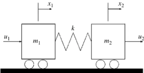
A single-axis, rest-to-rest maneuvering problem of flexible spacecraft used as a benchmark problem in many studies (Driessen 2000, Pao 1996, Liu and Wie 1992, Wie et al., 1993) is chosen as an example of the time-optimal control problem in this section. The system model, shown in Fig. 2(a), only with a scalar control input u1(t) is considered here.
Follow-ing the NLP formulation described in Section III, the optimal control can be defined as follows.
Minimize J0= dt 0 tf = tf (12) Subject to x1= x3 x2= x4 x3= u1 m1 – km1(x1– x2) x4= km 2(x1– x2) (13)
with initial states
xT
(0) = [0, 0, 0, 0]T
(14) where x1 and x2 are the positions of body 1 and body
2, respectively, the nominal parameters are m1 = m2
= k = 1 with appropriate units, and time is in seconds. The terminal state constraints and saturation con-straints on control are described as:
ψ1 = x1(tf) – 1 = 0 (15)
ψ2 = x2(tf) – 1 = 0 (16)
ψ3 = x3(tf) = 0 (17)
ψ4 = x4(tf) = 0 (18)
ψ5 = |u1| – 1 ≤ 0 (19)
Time-optimal control problems often occur in many practical control problems. In this case, the derivation of the PMP is complex and thus the de-tails are skipped. Following the procedure described in Section IV, users only need prepare two parameter files and user routines. Table 1 shows the user rou-tines of this problem. By applying the proposed method and suggested procedure, a solution as tf = 4.2178746
is obtained and the trajectories of the states and con-trol input are shown in Fig. 2(b). In this problem, the proposed solver also obtains three switching times of input control as 1.00266823, 2.10892571 and
3.21518969. Those results agree with the results ob-tained by Liu and Wie (1992).
As the numerical results show, OCP is success-fully converted into an NLP problem with the admis-sible control formulation and solved with the pro-posed method. The results show that the propro-posed method is applicable. According to the procedure suggested in this paper, users need not spend a vast amount of effort on programming in order to obtain solutions to problems. After formulating the prob-lems and writing the user-defined routines, the pro-posed solver can solve the problems easily.
VI. CONCLUSIONS
An optimal control problem solver, the OCP solver, based on the Sequential Quadratic Program-ming (SQP) method and integrated with many well-developed numerical routines is implemented in this paper. A systematic procedure for solving optimal control problems is also offered in this paper. A high-order nonlinear time-optimal control problem is used to demonstrate the capability of the OCP solver. The results show that the OCP solver can help engineers in solving optimal control problems with a system-atic and efficient procedure.
Fig. 2 Time-optimal rest-to-rest maneuvering problem
x1 m1 u1 m u2 2 k x2 1.2 1.0 0.8 0.6 0.4 0.2 0.0 0 1 2 3 Time (sec.) (i) State trajectories
(a) Two-mass-spring system model (Liu and Wie 1992)
(b) Numerical results 4 5 6 x2 x1 1.0 0.8 0.6 0.4 0.2 0.0 -0.2 -0.4 -0.6 -0.8 -1.0 0 1 2 3 Time (sec.) (ii) Control trajectories
4 5 6
u
732 Journal of the Chinese Institute of Engineers, Vol. 28, No. 4 (2005)
ACKNOWLEDGMENTS
The research reported in this paper, was supported by a the National Science Council Grant, Taiwan, R.O.C., NSC90-2212-E009-039, which is greatly appreciated.
NOMENCLATURE
b design variables
d(k)
descent direction defined in SQP algorithm
t0 start time
tf terminal time
u control variable vector
x state variable vector
H Hessian Matrix
N number of time intervals
P extended design variable vector
Ti the i-th time grid point
α step size of SQP algorithm
ε convergence parameter of SQP algorithm
REFERENCES
Bellman, R., 1957, Dynamic Programming, Princeton University Press, Princeton, NJ, USA.
Table 1 User routines for solving the Benchmark problem
// Parameters for numerical examples #define m1 1.0
#define m2 1.0 #define k 1.0
//Routine to calculate the integral term of the performance index or functional constraint.
void ffn(double *B, double *U, double *Z, double *T, double *F, int NV, int NU, int NEQ, int N, int NBJ) {
*F = 0.0; }
// Routine to calculate the first term of the performance index or functional constraint // or dynamic constraint.
void gfn(double *B, double *U, double *Z, double *T, double *G, int NV, int NU, int NEQ, int N, int NBJ) { switch (N) { case 0: *G = B[3]; /* B[3]:terminate time tf */ break; case 1: *G = Z[0] - 1.0; /* terminal constraints */ break; case 2: *G = Z[1] – 1.0; break; case 3: *G = Z[2] ; break; case 4: *G = Z[3] ; break; }; }
// Routine to calculate the state trajectory.
void hfn(double *B, double *U, double *Z, double *DZ, double *T, int NV, int NU, int NEQ) { DZ[0] = Z[2]; DZ[1] = Z[3]; DZ[2] = (U[0]/m1)-(k/m1)*(Z[0]-Z[1]); DZ[3] = (k/m2)*(Z[0]-Z[1]); }
Betts, J. T., 2000, “Very Low-Thrust Trajectory Op-timization Using a Direct SQP Method,” Journal
of Computational and Applied Mathematics, Vol.
120, pp. 27-40.
Cervantes, A., and Biegler, L. T., 2000, “A Stable Elemental Decomposition for Dynamic Process Optimization,” Journal of Computational and
Ap-plied Mathematics, Vol. 120, pp. 41-57.
Driessen, B. J., 2000, “On-Off Minimum-Time Con-trol with Limited Fuel Usage: Near Global Op-tima via Linear Programming,” Proceedings of
the American Control Conference, Chicago, IL,
USA, pp. 3875-3877.
Gill, P. E., Murray, W., and Saunders, M. A., 2002, “SNOPT: An SQP Algorithm for Large-Scale Constrained Optimization,” SIAM Journal on
Optimization, Vol. 12, No. 4, pp. 979-1006.
Hu, G. S., ONG, C. J., and Teo, C. L., 2002, “An Enhanced Transcribing Scheme for The Numeri-cal Solution of a Class of Optimal Control Problems,” Engineering Optimization, Vol. 34, No. 2, pp. 155-173.
Jaddu, H., and Shimemura, E., 1999, “Computational Method Based on State Parameterization for Solv-ing Constrained Nonlinear Optimal Control Problems,” International Journal of Systems
Science, Vol. 30, No. 3, pp. 275-282.
Liu, Q., and Wie, B., 1992, “Robust Time-Optimal Control of Uncertain Flexible Spacecraft,”
Jour-nal of Guidance, Control, and Dynamics, Vol. 15,
No. 3, pp. 597-604.
Pao, L. Y., 1996, “Minimum-Time Control Charac-teristics of Flexible Structures,” Journal of
Guidance, Control, and Dynamics, Vol. 19, No.
1, pp. 123-129.
Pontryagin, L. S., Boltyanskii, V. G., Gamkrelidze, R. V., and Mischenko, E. F., 1962, The
Math-ematical Theory of Optimal Processes, Wiley,
New York, USA.
Tseng, C. H., Liao, W. C., and Yang, T. C., 1996, “MOST 1.1 User’s Manual,” Technical Report
No. AODL-96-01, Department of Mechanical
Engineering, National Chiao Tung University, Taiwan, R.O.C..
Wie, B., Sinha, R., and Liu, Q., 1993, “Robust Time-Optimal Control of Uncertain Structural Dynamic Systems,” Journal of Guidance, Control, and
Dynamics, Vol. 16, No.5, pp. 980-983.
Manuscript Received: Jun. 07, 2004 Revision Received: Sep. 12, 2004 and Accepted: Oct. 20, 2004