I-Shou University Institutional Repository:Item 987654321/11819

全文

(1)義守大學資訊工程研究所博士論文 (24, 12, 8)葛雷碼之解碼. On the decoding of the (24, 12, 8) Golay code. 研究生：張新球指導教授：張肇健博士共同指導教授：林宗慶博士. 中華民國九十九年十二月.

(2) (24, 12, 8)葛雷碼之解碼 On the decoding of the (24, 12, 8) Golay code 研究生：張新球指導教授：張肇健博士共同指導教授：林宗慶博士. Student：Hsin-Chiu Chang Advisor：Dr. Trieu-Kien Truong Co-Advisor：Dr. Tsung-Ching Lin. 義守大學資訊工程研究所博士論文 A Dissertation Submitted to the Department of Information Engineering of I-Shou University in Partial Fulfillment of the Requirements for the Ph.D. Degree with a Major in Information Engineering December, 2010 Kaohsiung, Taiwan, Republic of China. 中華民國九十九年十二月.

(3)

(4)

(5) Dedication This dissertation is dedicated to my parents and is also dedicated to my family. Without whose sacrifices none of this would have been possible.. I.

(6) Acknowledgments I would like to express my sincere gratitude and the most appreciation to my advisor, Professor Trieu-Kien Truong (張肇健教授), and my co-advisor, Professor Tsung-Ching Lin (林宗慶教授), for their assistance and support during my study at I-Shou University. Without their guidance, continued encouragement, and a lot of ideas for solving certain tough and complicated problems, this dissertation would not have been completed. I am also grateful to my research member, Hung-Peng Lee ( 李鴻鵬 ), for his encouragement and many helpful discussions in my research. I would like to acknowledge the support and suggestions of the whole members of my dissertation committee, Dr. Cheng-Hong Yang (楊正宏教授), Dr. Chung-Nan Lee (李宗南教授), and Dr. Wen-Shyong Hsieh (謝文雄教授), for providing valuable discussions and suggestions. Finally, special thanks to my mother, my wife, and my children because they accompanied me and gave me continuous support and understanding on my research.. II.

(7) (24, 12, 8)葛雷碼之解碼. 研究生：張新球. 指導教授：張肇健博士共同指導教授：林宗慶博士. 義守大學資訊工程研究所博士班. 摘要由於具有高碼率，二元平方剩餘碼(binary quadratic residue)，也是循環碼中的一種很好的家族，是已知線性區塊碼中最強的一種碼。本論文的研究主題專注在二元系統(24, 12, 8)平方剩餘碼，或稱為(24, 12, 8)葛雷碼(Golay code)的解碼。一個改良的徵狀值移位暫存解碼演算法，稱為徵狀值-權重解碼演算法 (syndrome-weight decoding algorithm)，被提出來解碼三個錯及偵測四個錯的(24, 12, 8)葛雷碼。這個解碼方法也能被延伸去解二種其它的碼，例如(15, 5, 7)循環碼和(31, 16, 7)二元平方剩餘碼。這個提出的解碼演算法是利用循環碼的性質，徵狀值的權重(weight)，及減少大小查找表的徵狀值解碼器(syndrome decoder with a reduced-size lookup table)，來減少徵狀值及其所對應的共集首部(coset leaders)。這個方法在查找表(lookup table)的記憶體需求上導致一個顯著的減少。電腦模擬的結果證明本論文所提出的演算法的解碼速度比代數解碼演算法的解碼速度快 3.6 倍。. 關鍵詞：徵狀值,權重,錯誤類型,循環碼,葛雷碼 III.

(8) On the decoding of the (24, 12, 8) Golay code. Student：Hsin-Chiu Chang. Advisor：Dr. Trieu-Kien Truong Co-Advisor：Dr. Tsung-Ching Lin. Department of Information Engineering I-Shou University. Abstract Due to the high code rate, binary quadratic residue (QR) codes, also a nice family of cyclic codes, are among the most powerful known linear block codes. This research concentrates on the topics of decoding the binary systematic (24, 12, 8) QR codes or called (24, 12, 8) Golay code. An improved syndrome shift-register decoding algorithm, called the syndrome-weight decoding algorithm (SWDA), is proposed for decoding three possible errors and detecting four errors in the (24, 12, 8) Golay code. This method can also be extended to decode two other short codes, such as the (15, 5, 7) cyclic code and the (31, 16, 7) QR code. The proposed decoding algorithm makes use of the properties of cyclic codes, the weight of syndrome, and the syndrome decoder with a reduced-size lookup table (RSLT) in order to reduce the number of syndromes and their corresponding coset leaders. This approach results in a significant reduction in the memory requirement for the lookup table, thereby yielding a faster decoding algorithm. Simulation results show that the decoding speed of the proposed algorithm is approximately 3.6 times faster than that of the algebraic decoding algorithm (ADA). IV.

(9) Keywords: syndrome, weight, error pattern, cyclic code, Golay code.. V.

(10) Contents Dedication .................................................................................................................................I Acknowledgments................................................................................................................... II Abstract (Chinese)................................................................................................................ III Abstract (English) .................................................................................................................IV Contents..................................................................................................................................VI List of Figures .....................................................................................................................VIII List of Tables ..........................................................................................................................IX Chapter 1. Introduction ........................................................................................................ 1. 1.1 Background.................................................................................................................... 3 1.2 Organization of the Dissertation.................................................................................. 6 Chapter 2. Mathematical Preliminaries .............................................................................. 8. 2.1 The Basic Concepts of Finite Fields............................................................................. 8 2.2 The Structure of Linear Block Codes ........................................................................ 21 2.3 The General Theory of Cyclic Codes......................................................................... 24 2.3.1 The Properties of Cyclic Codes ........................................................................... 24 2.3.2 Encoding and Examples....................................................................................... 26 2.4 The Basic Properties of QR Codes............................................................................. 32 Chapter 3. Algebraic Decoding Algorithm of the Binary Systematic (23, 12, 7) Golay. Code ........................................................................................................................................ 36 3.1 Background of the Binary Systematic (23, 12, 7) Golay Code ................................ 36 3.2 Algebraic Decoding Algorithm Developed by Elia ................................................... 38 3.3 The Decoding of the Binary (24, 12, 8) Golay Code ................................................. 39 3.4 A Fast Method for Computing the Multiplication and Inverse in GF(2m)............. 40 Chapter 4. Syndrome-Weight Decoding Algorithm of the Binary Systematic (23, 12, 7). Golay Code............................................................................................................................. 42 4.1 Syndrome Decoder with a Reduced-Size Lookup Table .......................................... 42 4.2 The Proposed Syndrome-Weight Decoding Algorithm............................................ 47 4.2.1 Construction of the Refined Lookup Table........................................................ 48 4.2.2 Decoding Procedure of SWDA ............................................................................ 51 VI.

(11) Chapter 5. Simulation Results............................................................................................ 59. Chapter 6. Conclusions and Future Directions ................................................................ 61. Appendix A............................................................................................................................. 63 Appendix B............................................................................................................................. 80 Bibliography .......................................................................................................................... 84. VII.

(12) List of Figures Figure 1 The binary symmetric channel (BSC)........................................................................ 2 Figure 4.1 Flowchart of the proposed SWDA with RLT........................................................ 53. VIII.

(13) List of Tables Table 2.1 Representation of the elements of GF(24) generated by 4 +  + 1 = 0................. 16 Table 2.2 Representations of the elements of vectors over GF(24) ........................................ 18 Table 2.3 The codewords of binary systematic Hamming code ............................................. 23 Table 2.4 Hamming code is a cyclic code .............................................................................. 25 Table 2.5 Encoding by c(x) = m(x)g(x)................................................................................... 27 Table 2.6 Encoding by using Eq. (2.5) ................................................................................... 28 Table 2.7 Encoding by using Eq. (2.7) ................................................................................... 30 Table 2.8 Encoding by using Eq. (2.10) ................................................................................. 31 Table 2.9 The parameters of some binary QR codes .............................................................. 35 i. Table 3.1 The values of indices S ti  S 2j .............................................................................. 38 Table 4.1 Comparison of the syndrome number between RSLT and RLT in three different codes ............................................................................................................................ 51 Table 4.2 Comparison of the memory size between RSLT and RLT in three different codes (in bytes)............................................................................................................................ 51 Table 5.1 Comparison of the computational time among three different decoding algorithms (in µs)........................................................................................................................... 59 Table A.1a The syndromes corresponding to error patterns in the RSLT for (15, 5, 7) cyclic code .............................................................................................................................. 63 Table A.1b The syndromes in ascending order corresponding to error patterns in the RSLT for (15, 5, 7) cyclic code.................................................................................................... 64 Table A.2a The syndromes corresponding to error patterns in the RSLT for (23, 12, 7) Golay code .............................................................................................................................. 65 Table A.2b The syndromes in ascending order corresponding to error patterns in the RSLT for (23, 12, 7) Golay code.................................................................................................. 68 Table A.3a The syndromes corresponding to error patterns in the RSLT for (31, 16, 7) QR code .............................................................................................................................. 70 Table A.3b The syndromes in ascending order corresponding to error patterns in the RSLT for (31, 16, 7) QR code...................................................................................................... 75 Table B.1 The syndromes corresponding to error patterns in the RLT for (15, 5, 7) cyclic code ...................................................................................................................................... 80 Table B.2 The syndromes corresponding to error patterns in the RLT for (23, 12, 7) Golay code .............................................................................................................................. 80 Table B.3 The syndromes corresponding to error patterns in the RLT for (31, 16, 7) QR code IX.

(14) ...................................................................................................................................... 81. X.

(15) Chapter 1 Introduction An error-correcting code is an algorithm for expressing a sequence of numbers such that any errors which are introduced can be detected and corrected (within certain limitations) based on the remaining numbers. The study of error-correcting codes and the associated mathematics is known as coding theory. Error detection is much simpler than error correction and one or more "check" digits are commonly embedded in credit card numbers in order to detect mistakes. Early space probes like Mariner used a type of error-correcting code called a block code, and more recent space probes use convolution codes. Error correcting codes are also used in CD players, high speed modems, and cellular phones. Modems use error detection when they compute checksums, which are sums of the digits in a given transmission modulo some number. The ISBN used to identify books also incorporates a check digit. The codes mentioned in this dissertation will all be binary block codes. The word binary indicates that the messages to be sent will consist only of 1's and 0's. The set {1, 0} is therefore called the alphabet for these codes. The word block indicates that the code will consist of words-- containing 1's and 0's--of constant length, n. Since we will be sending messages with words containing letters from the Latin alphabet these words must first be encoded into binary. This is called source encoding. Likewise, source decoding must take place in the receiver of the destination. The length of a binary message word that the alphabet is encoded into is usually denoted by k. The following assumptions will be made in our discussion of error correcting codes. . All code words sent over the channel of length n consisting of 0's and 1's will be received as blocks of length n consisting of 0's and 1's. 1.

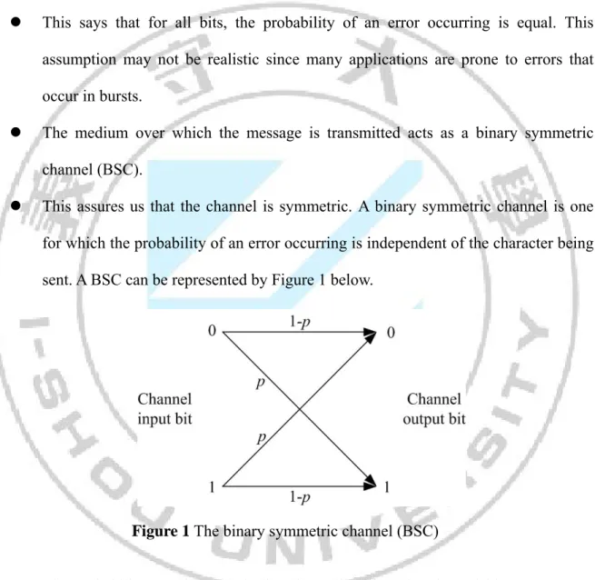
(16) . This is simply saying that a bit is not somehow lost in the channel along the way. It also rules out the possibility of erasures. (An erasure is a received bit that can not be interpreted as a 1 or a 0).. . The probability of an error occurring on any one bit is independent of the probability of an error occurring on any of its neighbors.. . This says that for all bits, the probability of an error occurring is equal. This assumption may not be realistic since many applications are prone to errors that occur in bursts.. . The medium over which the message is transmitted acts as a binary symmetric channel (BSC).. . This assures us that the channel is symmetric. A binary symmetric channel is one for which the probability of an error occurring is independent of the character being sent. A BSC can be represented by Figure 1 below.. Figure 1 The binary symmetric channel (BSC) . The probability, p, of a BSC is that the probability of a channel bit error occurs. Thus the probability that a 0 on the input causes a 1 at the output is p. The probability that the output should be a 0 when a 0 is input is therefore 1 – p.. ECC provides us with this ability. ECC allows us to receive a piece of signal, identify any errors, locate them, and correct them. Therefore, ECC have been found widespread. 2.

(17) applications in data networking, satellite communication and compact disks. Cyclic codes are a class of practical linear block codes. Cyclic codes are also an especially useful kind of ECCs, and Bose-Chaudhuri-Hocquenghem (BCH) codes and quadratic residue (QR) codes are especially useful kinds of cyclic codes. ECC theory is an important subject to study. In this dissertation we limit our attention to binary cyclic codes here. This means that the symbol alphabet consists of just two symbols which we denote 0 and 1 (GF(2)), that the receiver can correct a transmission error without asking the sender for more information or for a retransmission, and that the transmissions consist of a sequence of fixed length codewords. This place the codeword are vectors with entries in finite field GF(2), and the code is closed under vector addition and multiplication by the finite field. QR codes decoding algorithms are often used today in the error control system. QR code is also said to be cyclic if, for any code word, the cyclically shifted word is also a code word. The known QR codes have reasonably large minimum distances, so that most of them are the best known codes. Thus, there is a need for efficient algorithms to decode QR codes with more efficient decoding algorithm.. 1.1 Background Linear cyclic block codes are one of the most important families of the linear block codes and were first discussed in a series of technical notes and reports written between 1957 and 1959 by Prange at the Air Force Cambridge Research Labs. Linear cyclic block codes are the most easily implemented and therefore most widely used of the block codes. The famous QR codes, introduced by Prange in his 1957 report [1], are cyclic BCH codes with a high code rate close to 1/2 and generally have large minimum distances. Therefore, most of the known QR codes are the best-known codes [2], [3]. For the three-error-correcting cyclic code, the binary (15, 5, 7) cyclic code, the (23, 12, 7) QR code or Golay code [4], and the (31, 16, 7) QR code are often used in the decoding algorithm. Among them, the binary (23, 12, 7) Golay 3.

(18) code is the most famous cyclic code first discovered by Golay [4] in 1949. The 23-bit Golay code is a very useful code, particularly for applications when a parity bit is added to each word, to yield a half-rate code, called the (24, 12, 8) Golay code. It was utilized to provide error control on the voyager mission, see [5]. There are thirteen binary QR codes with code length less than 120, namely (7, 4 ,3) [6], (17, 9, 5), (23, 12, 7) [7-11], (31, 16, 7) [12-15], (41, 21, 9) [16, 17], (47, 24, 11) [18-21], (71, 36, 11) [22], (73, 37, 13) [23], (79, 40, 15) [22], (89, 45, 17) [24], (97, 49, 15) [22], (103, 52, 19) [25], and (113, 57, 15) [25]. Among those codes, (7, 4, 3) and (23, 12, 7) QR codes are the most famous. It is well known that all types of binary cyclic codes can be decoded by using Gröbner techniques up to their true minimum distance. In particular, a Gröbner technique for decoding the binary BCH codes is described in [26, pp. 69-91]. The key idea behind this technique is a systematic application of algorithmic procedures of Gröbner bases to obtain the error-location polynomial, denoted by L(z). The disadvantage of the Chen-Reed-Helleseth-Truong (CRHT) [27] algorithm is that it needs the process of transforming a set of syndrome polynomials F to the reduced Gröbner basis of the ideal <F> generated by F with respect to the purely lexicographical order to automatically converges to L(z). It follows from [28] that Buchberger’s algorithm for generating Gröbner bases is the most computationally intensive part of the CRHT algorithm. Therefore, it is very difficult to find the upper bound in the running time of algorithm 2 of [27] used to generate Gröbner bases except for some special cases. To overcome this, one needs to develop a simpler algorithm for the special polynomial set F. This is an important near-term problem of future study. Several decoding techniques have been developed to decode the Golay code. In 1987, a fast algebraic decoding algorithm developed by Elia [7] for the (23, 12, 7) Golay code was utilized to correct the three possible errors. Latterly, another decoding approach, called the shift-search decoding procedure [8], was developed to decode the binary Golay code. As 4.

(19) shown in [8], this shift-search procedure compares favorably in complexity and speed with Elia’s decoding method. The algebraic technique was shown to be slightly faster than the shift-search procedure. It is of interest to note that Elia’s decoding algorithm is simpler for the one- or two-error case, but it will become slower in decoding three errors because the computation complexity in D1/3 increases rapidly. During several decades, some other algebraic decoding algorithms were proposed. For example, Reed et al. [12, 16] used the algebraic with Sylvester resultant method or Gröbner bases method [27] to solve non-linear, multivariate equations obtained from the Newton identities. Also, the algebraic algorithm with inverse-free Berlekamp–Massey (BM) algorithm was developed by Truong et al. [22, 25] and Chen et al. [19] to determine the error-locator polynomial and to find out the error positions. These algebraic decoding algorithms definitely required a large number of additions and multiplications over a finite field. It causes the time delay in decoding procedures and is rather complicated to implement in the digital circuits. For some non-algebraic syndrome decoding methods, such as the syndrome decoder [5] and Meggitt decoder [29] are two well-known syndrome decoders or table lookup decoders, which apply in principle to any cyclic code. Basically, these two syndrome decoders result in minimum both decoding delay and error probability. Obviously, one error detection and correction circuit is relatively simple to implement. However, the implementation complexity of the error pattern detection circuit and the size of the lookup table for the syndrome decoder will be increased rapidly when the length of codeword n increases. The arithmetic decoding algorithm [5] is also a well-known decoder for decoding the (24, 12, 8) Golay code, whereas, this arithmetic decoder has some disadvantages. First, this arithmetic decoder can only decode self-dual based codes. Second, it can only correct three errors or fewer errors. Finally, it needs to compute a lot of matrix multiplications and additions for correcting up to three errors and detecting four errors, thereby increasing the decoding time.. 5.

(20) With a view to correcting more errors, Chase [30] used the hard decision decoder and the channel measurement information, i.e., reliability, to develop the decoding algorithms for block codes. However, the incurred hard-decoding complexity could be an issue for the decoding time. By extending the idea of the bit-error probability estimate [31], Su et al. [32-34] developed the new algorithm to correct up to four errors. Through their simulation results, the method developed by Su et al. achieves a better percentage of successful decoding for four errors at the variable signal-to-noise ratio (SNR) than Lu et al.’s method [35]. However, the decoding speed of the method based on the algebraic decoding algorithm developed by Elia [7] is slower than Lu et al.’s algorithm. In this dissertation, in order to develop a much smaller lookup table than RSLT given in [5], a new decoding algorithm called the syndrome-weight decoding algorithm (SWDA) is proposed to decode up to three possible errors in the (15, 5, 7) cyclic code, the (23, 12, 7) Golay code, and the (31, 16, 7) QR code. The algorithm can be extended to detect four errors in the (24, 12, 8) Golay code and the (32, 16, 8) QR code. It is based on the cyclic code properties, the syndrome weight, and the syndrome decoder with a RSLT. The refined lookup table (RLT) proposed in the SWDA consists of only 42 syndromes and their corresponding coset leaders (or called representative error patterns) for decoding the (23, 12, 7) Golay code. This leads to reduce the memory size, which renders this new decoding algorithm to be quite practical.. 1.2 Organization of the Dissertation The rest of the dissertation is organized as follows. Chapter 2 gives a brief overview of the mathematic background of the linear block codes and binary QR codes. An improvement of the algebraic decoding of the binary (23, 12, 7) Golay code is described in Chapter 3. Chapter 4 develops a syndrome-weight decoding algorithm for decoding the binary (23, 12, 7) 6.

(21) Golay code. Computer simulation results for the proposed SWDA and the ADA given in [7] are shown in Chapter 5. Finally, a few short remarks and conclusions for the proposed decoding scheme are summarized in Chapter 6.. 7.

(22) Chapter 2 Mathematical Preliminaries The purpose of this chapter is to provide the reader some of the basic concepts of algebra that will be needed for the study of QR codes.. 2.1 The Basic Concepts of Finite Fields Algebraic structure plays an important role in mathematical background of the binary QR codes. First we give the definitions of the commutative group, ring, and field [5].. Definition 2.1 A group G is a set of elements for which an operation is defined and used for the following four axioms. Let a, b and c be elements of the group and let “·” denote the operation in the group operation which can be any of +,  etc, for convenience. (1) Closure: for any a, c  G, a·c  G. (2) Associativity: for any a, b, c  G, a·(b·c) = (a·b)·c. (3) Identity: there is an identity element e  G such that for all a  G, a·e = e·a = a. (4) Inverse: for any a  G, there exists an inverse a-1  G such that a-1·a = a·a-1 = e. A group is said to be abelian (or commutative) if it also satisfies (5) Commutative law: a·b = b·a for all a, b  G.. The group operation for a commutative group is usually represented using the symbol “+”, and the group is sometimes said to be “additive” The group operation for a commutative group is usually represented using the symbol “·”, and the group is sometimes said to be. 8.

(23) “multiplicative”.. Definition 2.2 The number of elements in a group G is called the order of the group G, denoted G.. Definition 2.3 Let g be an element in the group G with operation “·”. The order of a group element g is the smallest positive integer ord(g) such that gord(g) is the group identity element.. Example 2.1 A group G of order 6 is G = {1, 2, 3, 4, 5, 6} under modulo 7 multiplication. The following table completely defines the group operation and orders of group elements. ·. 1. 2. 3. 4. 5. 6. 1 2 3 4 5 6. 1 2 3 4 5 6. 2 4 6 1 3 5. 3 6 2 5 1 4. 4 1 5 2 6 3. 5 3 1 6 4 2. 6 5 4 3 2 1. element order 1 2 3. element order. 1 3 6. 4 5 6. 3 6 2. Definition 2.4 Let S be a subset of the group G. If for all a and b in S, c = a·b-1 is also in S, then S is said to be a subgroup of G. This means that a subset of G is a subgroup if it exhibits closure and contains the necessary inverses. All other group properties are inherited from G. A subgroup is this itself a group. A subgroup S is said to be a proper subgroup if G if S  G, but S  G.. 9.

(24) Definition 2.5 Let S be a subgroup of G with operation “+”. A left coset of S in G is a subset of G whose elements can be expressed as x + S = {x + s, s  S}. A right coset of S in G is a subset of G whose elements can be expressed as S + x = {s + x, s  S}. If G is commutative, every left coset x + S is identical to every right coset S + x. They will simply be referred to as cosets.. Example 2.2 . The group of integers G under modulo 9 addition contains the proper subgroup S = {0, 3, 6}. The distinct cosets of S in G are {0, 3, 6}, {1, 4, 7}, and {2, 5, 8}.. . The group of integers G under modulo 16 addition contains the proper subgroup S = {0, 4, 8, 12}. The distinct cosets of S in G are {0, 4, 8, 12}, {1, 5, 9, 13}, {2, 6, 10, 14}, and {3, 7, 11, 15}.. Theorem 2.1 The distinct cosets of a subgroup S in a group G are disjoint.. Theorem 2.2 (Lagrange’s Theorem) If S is a subgroup of G, then ord(S)ord(G). The group, as explained so far, includes only an algebra operation. Considering algebra operations with two operations there are operators such as + and ·.. Definition 2.6 Rings and Fields: If a set R is a ring, it satisfies the statements. (1) R is an abelian group under addition. (2) R is closed under multiplication. (3) R is associative under multiplication. (4) Multiplication is distributive with respect to addition, that is, for any a, b, c  R,. a·(b+c) = a·b + a·c, (a+b)·c = a·c + b·c. 10.

(25) (5) There is multiplicative identity, denotes 1  R, for any a  R, a·1 = 1·a = a. (6) Commutatively: For any a, b  R, a·b = b·a  R. (7) Multiplicative inverse: for any a  R, a  0, there exists a-1  R such that a·a-1 = a-1·a = 1. A ring R satisfying statement (6) is called commutative ring. A ring R satisfying statement (6) and (7) is called a field.. We usually write a·b as ab. A field can also be defined as a commutative ring with identity in which every element has a multiplicative inverse. Field of finite order (cardinality) is particularly interesting to coding theorists. Finite fields were discovered by Evariste Galois and are thus known as Galois field. A Galois field of order q is usually denoted GF(q). The Galois field is briefly described in next section.. Definition 2.7 Let a, b and n > 1 be integers. We say that a and b are congruent modulo n, written as a  b (mod n), if n(a – b); i.e., n divides a – b.. Example 2.3 1.. 23  2 mod 7 and -2  19 mod 7.. 2.. Integer modulo n groups the infinite set of integers into n distinct equivalence classes, so the equivalence classes of integers under modulo 4 are shown below: 0 = {…, -12, -8, -4, 0, 4, 8, 12, …}. 1 = {…, -11, -7, -3, 1, 5, 9, 13, …}. 2 = {…, -10, -6, -2, 2, 6, 10, 14, …}. 3 = {…, -9, -5, -1, 3, 7, 11, 15, …}.. Theorem 2.3 The integers {0, 1,…, p-1}, where p is a prime, form the field GF(p) under modulo p addition and multiplication.. 11.

(26) Example 2.4 Let F be the set of integer modulo 11; that is, F = {0, 1, 2, 3, 4, 5, 6, 7, 8, 9, 10}. Construct the finite field GF(11) under modulo 11 addition and multiplication, and list the order for every element of GF(11).. +. 0. 1. 2. 3. 4. 5. 6. 7. 8. 9. 10. 0 1 2 3 4. 0 1 2 3 4. 1 2 3 4 5. 2 3 4 5 6. 3 4 5 6 7. 4 5 6 7 8. 5 6 7 8 9. 6 7 8 9 10. 7 8 9 10 0. 8 9 10 0 1. 9 10 0 1 2. 10 0 1 2 3. 5 6 7 8 9 10. 5 6 7 8 9 10. 6 7 8 9 10 0. 7 8 9 10 0 1. 8 9 10 0 1 2. 9 10 0 1 2 3. 10 0 1 2 3 4. 0 1 2 3 4 5. 1 2 3 4 5 6. 2 3 4 5 6 7. 3 4 5 6 7 8. 4 5 6 7 8 9. ·. 0. 1. 2. 3. 4. 5. 6. 7. 8. 9. 10. 0 1 2 3 4 5. 0 0 0 0 0 0. 0 1 2 3 4 5. 0 2 4 6 8 10. 0 3 6 9 1 4. 0 4 8 1 5 9. 0 5 10 4 9 3. 0 6 1 7 2 8. 0 7 3 10 6 2. 0 8 5 2 10 7. 0 9 7 5 3 1. 0 10 9 8 7 6. 6 7 8 9 10. 0 0 0 0 0. 6 7 8 9 10. 1 3 5 7 9. 7 10 2 5 8. 2 6 10 3 7. 8 2 7 1 6. 3 9 4 10 5. 9 5 1 8 4. 4 1 9 6 3. 10 8 6 4 2. 5 4 3 2 1. 12.

(27) element order 1 2 3 4 5. element order. 1 10 5 5 5. 6 7 8 9 10. 10 10 10 5 1. We examine some of the basic properties of Golois fields. The application of Golois fields is very important in the coding system. Finite fields of prime order are quite easy to construct. However, finite fields GF(q) do not exist for all values of q. q must equal pm, where. p is a prime positive integer and m is a positive integer. In this dissertation, we restrict p = 2.. Definition 2.8 Let  be an element in GF(q). The order of  (written ord()) is the smallest positive integer m such that m = 1. This definition is identical to that for the order of an element in a group. It should be noted, however, that for the case of the Galois field element, “order” is defined using the multiplicative operation and not the additive operation. We first note that the order of an arbitrary element  in the Glaois field GF(q) must be a divisor of (q–1).. Theorem 2.4 If m = ord() for some   GF(q), then m(q–1).. Definition 2.9 (The multiplicative structure of Galois field) Consider the Galois field GF(q). 1.. If m does not divide (q–1), then there are no elements of order m in GF(q).. 2.. If m (q–1), then there are (m) elements of order m in GF(q), where the Euler  function ( m) evaluated at an integer m is the number of integers in the set {1,…,. m–1} that are relatively prime to m (i.e., share no common divisors other than one).. 13.

(28) Definition 2.10 An element with order (q–1) in GF(q) is called a primitive element in GF(q). Every field GF(q) thus contains at least one primitive element . Let  be a primitive element in GF(q) and consider the sequence 1, , 2,…, q-2,  q-1,  q,…. By Definition 2.9,.  q-1 is the first positive power of  in the sequence to repeat the value 1. Therefore, all nonzero elements in GF(q) can be represented as (q–1) consecutive powers of a primitive element .. Example 2.5 In the Example 2.4, ord(3) = 6 and ord(5) = 6. Thus, field elements 3 and 5 are primitive elements. Consider the consecutive powers of 3: 31 = 3, 32 = 2, 33 = 6, 34 = 4, 35 = 5, 36 = 1. The powers of 3 generate all the nonzero field elements.. Theorem 2.5 The order q of a Galois field GF(q) must be a power of a prime. The set of all polynomials with coefficients forms a commutative ring with identity under standard polynomial addition and multiplication. This ring is usually denoted GF(q)[x] or Fq[x]. The notation GF(q)[x] is used to denote the collection of all polynomials anxn + ··· +. a1x +a0 of arbitrary degree with coefficients {ai} in the finite field GF(q). The coefficient operations are performed using the operations for the field from which the coefficients were taken. For example, polynomial with binary coefficients in GF(2), (x5 + x2) + (x2 + x + 1) = x5 + 2x2 + x + 1 = x5 + x + 1.. Definition 2.11 (Irreducible polynomials) A polynomial f(x) is irreducible if it cannot be expressed as a product of lower degree polynomials. These polynomials are also called prime polynomials.. 14.

(29) Example 2.6 All irreducible polynomials of degree 2, 3, and 4 in GF(2)[x] are x2 + x + 1, x3 + x + 1, x3 + x2 + 1, x4 + x + 1, x4 + x3 + 1, and x4 + x3 + x2 + x + 1.. Definition 2.12 (Primitive polynomials) An irreducible polynomial p(x)  GF(p)[x] of degree m is said to be primitive if the smallest positive integer n for which p(x) divides xn – 1 is n = pm – 1; that is, p(x)xp. m–1. – 1.. A primitive polynomial p(x)  GF(p)[x] is always irreducible in GF(p)[x], but irreducible polynomial are not always primitive.. Example 2.7 Irreducible polynomials and Primitive polynomials 1.. x3 + x + 1 is irreducible in GF(2)[x]. Also, x3 + x + 1 is primitive in GF(2)[x], for the smallest polynomial of the form xn – 1 for which it is a divisor is x7 – 1 (7 = 23 – 1).. 2.. x4 + x + 1 is irreducible in GF(2)[x]. Also, x4 + x + 1 is primitive in GF(2)[x], for the smallest polynomial of the form xn – 1 for which it is a divisor is x15 – 1 (15 = 24 – 1). x4 + x3 + x2 + x + 1 is irreducible in GF(2)[x], but is a factor of x5 – 1 and thus not primitive in GF(2)[x].. 3.. x11 + x2 + 1 is irreducible in GF(2)[x]. Also, x11 + x2 + 1 is primitive in GF(2)[x], for the smallest polynomial of the form xn – 1 for which it is a divisor is x2047 – 1 (2047 = 211 – 1).. Theorem 2.6 The roots {j} of an mth-degree primitive polynomial p(x)  GF(p)[x] have order pm – 1.. Example 2.8 15.

(30) Primitive polynomials p(x) = x11 + x2 + 1  GF(2)[x] has 11 roots, say {1, 2, 3, 4, 5,. 6, 7, 8, 9, 10, 11}. Let 1 = 2, 2 = 4, 3 = 16, 4 = 256, 5 = 160, 6 = 1064, 7 = 1605, 8 = 158, 9 = 380, 10 = 1530, 11 = 1987. The order of all roots is 211 – 1 = 2047. Given that  is a root of Primitive polynomials p(x) and  has order pm – 1, the pm – 1 consecutive powers of  form a multiplicative group of order pm – 1. The multiplication operation is performed by adding the exponents of the power of  modulo pm – 1. These exponential representations can be reexpressed by reducing the sequence of powers of  modulo the primitive polynomial. The pm – 1 consecutive powers of  can thus be shown to be the nonzero elements of the field GF(pm). The roots of a mth-degree primitive polynomial in GF(p)[x] are primitive elements in GF(pm).. Example 2.9 Let  be a root of primitive polynomials p(x) The representation of the field GF(24), constructed by the p(x) = x4 + x + 1, is shown in Table 2.1. Table 2.1 Representation of the elements of GF(24) generated by 4 +  + 1 = 0 Exponential representation.  1 2 3 4 5 6 7 8 9 10 11 12 13 14 0. 0. Polynomial representation = = = = = = = = = = = = = = = =. 1.  2 3 4 =  + 1 5 = 2 +  6 = 3 +2 7 = 4 + 3 = 3 +  + 1 8 = 4 + 2 +  = 2 + 1 9 = 3 +  10 = 4 + 2 = 2 +  + 1 11 = 3 + 2 +  12 = 4 +3 + 2 = 3 + 2 +  + 1 13 =4 + 3 + 2 +  = 3 + 2 + 1 14 = 4 + 3 +  = 3 + 1 0. 16.

(31) Multiplication is easily performed through the use of the exponential representations. The exponents of the two elements being multiplied together are added together modulo (24 – 1) to obtain the exponent of the product. Multiplication can also be performed through the polynomial representation. If a + b have the polynomial representations a22 + a1 + a0 and. b22 + b1 + b0, respectively, then (a+b) mod 15 has polynomial representation (a22 + a1 + a0) (b22 + b1 + b0) modulo (4 +  + 1). Addition can also be performed using the polynomial representation. For example, computing 9 + 3 = (3 + ) + 3 =  in GF(24), the polynomials are then summed to obtain a third polynomial and re-expressed as a power of . One element operated on itself (1+1) is zero. Then multiplication is illustrated as 9·13 = 9+13 = 22 mod 15 = 7. We can find that the addition is actually an XOR operation and the multiplication is the exponential of the operation.. The polynomial representation for a finite field GF(pm) has coefficients in the GF(p). Clearly, GF(pm) can thus be interpreted as a vector space over GF(p). Table 2.1 can also represent as vectors over GF(24) and is shown in Table 2.2.. 17.

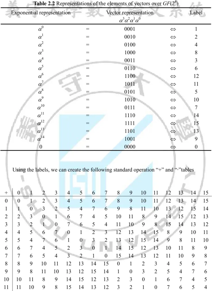
(32) Table 2.2 Representations of the elements of vectors over GF(24) Exponential representation. Vector representation. Label. . 3 2 1 0.  1 2 3 4 5 6 7 8 9 10 11 12 13 14 0. = = = = = = = = = = = = = = = =. 0.                . 0001 0010 0100 1000 0011 0110 1100 1011 0101 1010 0111 1110 1111 1101 1001 0000. 1 2 4 8 3 6 12 11 5 10 7 14 15 13 9 0. Using the labels, we can create the following standard operation “+” and “·”tables. + 0 1 2 3 4 5 6 7 8 9 10 11 12 13 14 15. 0 0 1 2 3 4 5 6 7 8 9 10 11 12 13 14 15. 1 1 0 3 2 5 4 7 6 9 8 11 10 13 12 15 14. 2 2 3 0 1 6 7 4 5 10 11 8 9 14 15 12 13. 3 3 2 1 0 7 6 5 4 11 10 9 8 15 14 13 12. 4 4 5 6 7 0 1 2 3 12 13 14 15 8 9 10 11. 5 5 4 7 6 1 0 3 2 13 12 15 14 9 8 11 10. 6 6 7 4 5 2 3 0 1 14 15 12 13 10 11 8 9. 7 7 6 5 4 3 2 1 0 15 14 13 12 11 10 9 8 18. 8 8 9 10 11 12 13 14 15 0 1 2 3 4 5 6 7. 9 9 8 11 10 13 12 15 14 1 0 3 2 5 4 7 6. 10 10 11 8 9 14 15 12 13 2 3 0 1 6 7 4 5. 11 11 10 9 8 15 14 13 12 3 2 1 0 7 6 5 4. 12 12 13 14 15 8 9 10 11 4 5 6 7 0 1 2 3. 13 13 12 15 14 9 8 11 10 5 4 7 6 1 0 3 2. 14 14 15 12 13 10 11 8 9 6 7 4 5 2 3 0 1. 15 15 14 13 12 11 10 9 8 7 6 5 4 3 2 1 0.

(33) ·. 0. 1. 2. 3. 4. 5. 6. 7. 8. 9. 10. 11. 12. 13. 14. 15. 0 1 2 3 4 5 6 7 8 9 10 11. 0 0 0 0 0 0 0 0 0 0 0 0. 0 1 2 3 4 5 6 7 8 9 10 11. 0 2 4 6 8 10 12 14 3 1 7 5. 0 3 6 5 12 15 10 9 11 8 13 14. 0 4 8 12 3 7 11 15 6 2 14 10. 0 5 10 15 7 2 13 8 14 11 4 1. 0 6 12 10 11 13 7 1 5 3 9 15. 0 7 14 9 15 8 1 6 13 10 3 4. 0 8 3 11 6 14 5 13 12 4 15 7. 0 9 1 8 2 11 3 10 4 13 5 12. 0 10 7 13 14 4 9 3 15 5 8 2. 0 11 5 14 10 1 15 4 7 12 2 9. 0 12 11 7 5 9 14 2 10 6 1 13. 0 13 9 4 1 12 8 5 2 15 11 6. 0 14 15 1 13 3 2 12 9 7 6 8. 0 15 13 2 9 6 4 11 1 14 12 3. 12 13 14 15. 0 0 0 0. 12 13 14 15. 11 9 15 13. 7 4 1 2. 5 1 13 9. 9 12 3 6. 14 8 2 4. 2 5 12 11. 10 2 9 1. 6 15 7 14. 1 11 6 12. 12 6 8 3. 15 3 4 8. 3 14 10 7. 4 10 11 5. 8 7 5 10. A vector space may be represented by a polynomial which can be expressed as. f ( x)    f 2 x 2  f1 x  f 0 , where x is called an unknown and the coefficients fi are in GF(q). The polynomail f ( x)  f n 1 x n 1    f 2 x 2  f 1 x  f 0 with the degree n–1 or less can rewrite as an n-tuple vector (fn-1,…,f1, f0). This correspondence is illustrated as follows.. Example 2.10. Two polynomials f(x) and g(x) are over GF(24), which means the coefficients of f(x) and g(x) are in GF(24), and let. f(x) = 9x2 + 6x + 1 = 14x2 + 5x + 0  f = (9, 6, 1), g(x) = 11x2 + 8x + 2 = 7x2 + 3x +   g = (11, 8, 2). Then, f(x) + g(x) = (14 + 7)x2 + (5 + 3)x + (0 + ) = x2 + 11x + 3  f + g = (9, 6, 1) + (11, 8, 2) = (9+11, 6+8, 1+2) = (2, 14, 3), 19.

(34) and f(x)·g(x) = (14x2 + 5x + 0)(7x2 + 3x + ) = 6x4 + 7x3 + 3x2 + 2x +   f·g = (9, 6, 1)·(11, 8, 2) = (12, 11, 8, 4, 2).. Definition 2.13 Let  be an element in GF(pm). We call the monic polynomial of smallest. degree, which has coefficients in GF(p) and  as a root, the minimal polynomial of .. Example 2.11. We will find the minimal polynomials of all the elements of GF(23). First of all, the elements 0 and 1 will have minimal polynomials x and x + 1 respectively. We construct GF(23) using the primitive polynomial x3 + x + 1 which has the primitive element  as a root. There are 4 monic 2nd degree polynomials over GF(23), x2, x2 + 1, x2 + x, and x2 + x + 1. The first three polynomials can be factored and so have roots in GF(2), but these elements have already been taken care of. The last quadratic has no roots in GF(23) which we can determine by substituting the elements into this polynomial. Consequently, any other minimal polynomials will have to have degree at least 3. The minimal polynomial of  is therefore the primitive polynomial x3 + x + 1. This polynomial also has two other roots, 2 and 4 (which we can determine by substitution of the field elements). The three elements 3, 6 and 5 all satisfy the cubic x3 + x2 + 1, so it must be the minimal polynomial for these elements.. Element. Minimal Polynomial. 0 1. x x+1 3 x +x+1 x3 + x2 + 1. , 2, 4 3, 6, 5. 20.

(35) Theorem 2.7 Let a(x) be the minimal polynomial of an element  in GF(pm). Then:. (i). a(x) is irreducible.. (ii) if  is a root of a polynomial f(x) with coefficients in GF(p), then a(x) divides f(x); that is, a(x)f(x). m. (iii) a(x) divides xp – x. (iv) if a(x) is primitive, then its degree is m. In any case, the degree of a(x) is equal or less to m; that is, deg{a(x)}  m.. 2.2 The Structure of Linear Block Codes Cyclic code is a kind of linear block bode. Linear block codes are the most easily implemented and therefore most widely used of the block codes. By definition they form vector subspaces over finite fields and they have a lot of interesting properties.. Definition 2.14 An (n, k) block code C uniquely maps a block of information symbols of. length k, i.e., m = (mk-1,…, m1, m0) to a codeword of length n, i.e., c = (cn-1,…, c1, c0). The number of redundancy symbols is n – k. The ratio R = k/n is the code rate. The encoding process consists of breaking up the data stream into blocks, and mapping these blocks onto codewords in C. This mapping is usually one-to-one, ensuring that the encoding process can be reversed at the receiver and the original data block recovered. If the symbols in the data stream can take on any value in GF(q), then the collection of all possible k-tuples m = (mk-1,…, m1, m0) forms a vector space over GF(q). That is, there are qk codewords in C, and all-zero vector is a codeword.. 21.

(36) Definition 2.15 Let a and b are codewords in a block code C. If C is a linear code, then any. linear combination of a and b are codewords in C.. Definition 2.16 The dimension of a linear code is the dimension of the corresponding vector. space.. Definition 2.17 The Hamming norm or weight of a binary vector a = (an-1,…, a0) is. designated by w(a).. Definition 2.18 The Hamming distance or distance between two binary vectors a and b is. defined by d(a, b) = w(a + b).. Definition 2.19 The minimum distance d of a code C is the minimum distance between any. two different codewords, i.e., d  min {d (a, b)} . a,bC,a  b. Since C is a vector subspace over GF(q), the linear combination of any set of codewords is a codeword. The minimum distance of linear code is equal to the weight of the lowest weight nonzero codeword. The (n, k, d) is used to denote a linear code C such that . n is the length of the codewords.. . k is the number of data symbols in a codeword.. . d is the minimum distance in C.. Example 2.12. Create the codewords of the binary systematic (7, 4, 3) Hamming code. The generator matrix is. 22.

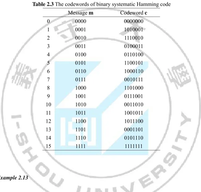
(37) 1 0 G 1  1. 1 0 1 0 0 0 1 1 0 1 0 0 . 1 1 0 0 1 0  0 1 0 0 0 1. There are 16 codewords for this linear code and they are shown as below. Table 2.3 The codewords of binary systematic Hamming code 0 1 2 3 4 5 6 7 8 9 10 11 12 13 14 15. Message m. Codeword c. 0000 0001 0010 0011 0100 0101 0110 0111 1000 1001 1010 1011 1100 1101 1110 1111. 0000000 1010001 1110010 0100011 0110100 1100101 1000110 0010111 1101000 0111001 0011010 1001011 1011100 0001101 0101110 1111111. Example 2.13. The linear combination of any set of codewords in Table 2.3 is also a codeword in Table 2.3. Let c1 + c2 + c3 + c4 = c4, then the resulting codeword c4 is also a codeword. Let c10 + c12, then the resulting codeword c6 is also a codeword.. 23.

(38) 2.3 The General Theory of Cyclic Codes Cyclic codes are a special class of error correcting codes. Within the family of cyclic codes there are certain special families of codes that are extremely powerful. These include the QR, BCH, and Reed-Solomon codes.. 2.3.1 The Properties of Cyclic Codes. Definition 2.20 A q-ary (n, k) linear code C is called a cyclic code if every cyclic shift of a code vector c = (cn-1, cn-2,…, c1, c0) in C is also a code vector c’ = (cn-2, cn-3,…, c0, cn-1) in C. If the codeword c’ is the right cyclic shift of the codeword c  C, then c’(x) = x·c(x) mod (xn – 1)  C. This can be seen as follows.. x·c(x)  x·(cn-1x n-1 + cn-2xn-2 + … + c1x + c0) mod (xn – 1)  (cn-1x n + cn-2xn-1 + … + c1x2 + c0x) mod (xn – 1)  (cn-2x n-1 + cn-3xn-2 + … + c0x + c n-1) mod (xn – 1)  c’(x) mod (xn – 1) In a similar manner, the cyclic shifts of c and the associated polynomials is represented as follows. c = (cn-1,…, c1, c0)  c(x) = cn-1x n-1 + … + c1x + c0 c’ = (cn-2,…, c0, cn-1)  c’(x) = cn-2x n-1 + … + c0x + cn-1 c’’ = (cn-3,…, cn-1, cn-2)  c’(x) = cn-3x n-1 + … + cn-1x + cn-2 . c(n-1) = (c0,…, c2, c1)  c’(x) = c0x n-1 + … + c2x + c1. 24. (2.1).

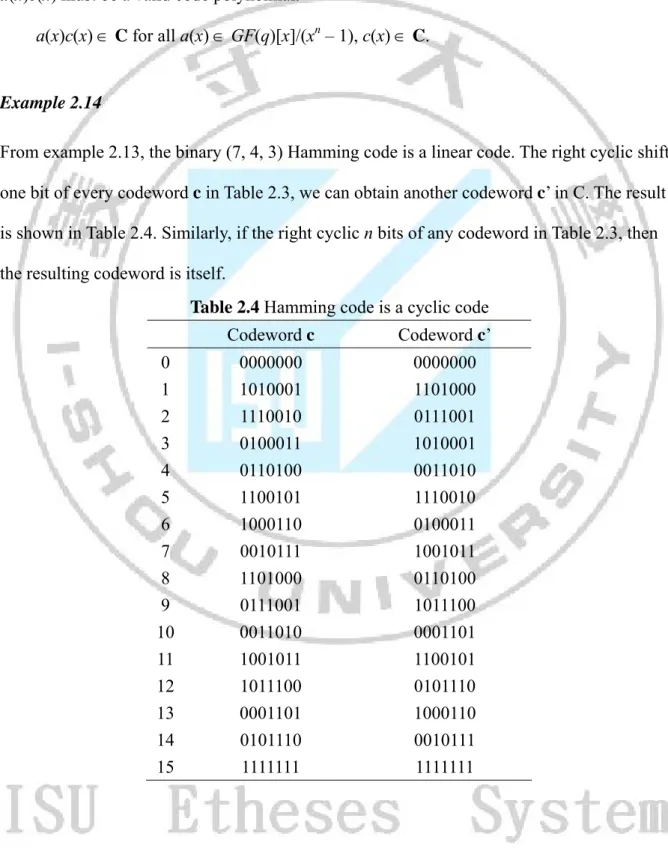
(39) Theorem 2.8 C is a q-ary linear cyclic code of length n if and only if the code polynomials in C form an ideal in GF(q)[x]/(xn – 1). Let a(x) = an-1x n-1 + … + a1x + a0 be an arbitrary polynomial in GF(q)[x]/(xn – 1). The product a(x)c(x) is a linear combination of cyclic shifts of c. Since C forms a vector space,. a(x)c(x) must be a valid code polynomial. a(x)c(x)  C for all a(x)  GF(q)[x]/(xn – 1), c(x)  C.. Example 2.14. From example 2.13, the binary (7, 4, 3) Hamming code is a linear code. The right cyclic shift one bit of every codeword c in Table 2.3, we can obtain another codeword c’ in C. The result is shown in Table 2.4. Similarly, if the right cyclic n bits of any codeword in Table 2.3, then the resulting codeword is itself. Table 2.4 Hamming code is a cyclic code 0 1 2 3 4 5 6 7 8 9 10 11 12 13 14 15. Codeword c. Codeword c’. 0000000 1010001 1110010 0100011 0110100 1100101 1000110 0010111 1101000 0111001 0011010 1001011 1011100 0001101 0101110 1111111. 0000000 1101000 0111001 1010001 0011010 1110010 0100011 1001011 0110100 1011100 0001101 1100101 0101110 1000110 0010111 1111111. 25.

(40) Theorem 2.9 Let C be a q-ary (n, k) linear cyclic code. 1.. Within the set of code polynomials in C there is a unique monic polynomial g ( x )  i 0 g i xi  g n  k x n  k    g 1 x g 0 with minimal degree (n–k) < n and g0  nk. 0, g(x) is called the generator polynomial of C. 2.. Every code polynomial c(x) in C can be expressed uniquely as c(x) = m(x)g(x), where g(x) is the generator polynomial of C and m(x) is a polynomial of degree less than k in GF(q)[x].. 3.. The generator polynomial g(x) of C is a factor of xn – 1 in GF(q)[x].. 2.3.2 Encoding and Examples The encoding of the cyclic codes is very important in FEC. In general, there are two kinds of encoding methods to generate codewords. In this section, we briefly describe two encoding processes of cyclic codes. Let m( x)  i 0 mi xi m k 1 x k 1    m1 x  m0  m = (mk-1,…, m1, m0), from the last k 1. theorem the codeword is obtained by. c(x) = m(x)g(x) = cn-1x n-1 + … + c1x + c0  c = (cn-1,…, c1, c0). (2.2). Definition 2.21 An encoder for a block code is systematic if the first k bits of every codeword are the same k bits of the message words; otherwise, it is called non-systematic.. Example 2.15. Let g(x) = x3 + x + 1 be the generator polynomial of the binary (7, 4, 3) Hamming code. Let m(x) = 1 be a message polynomial. Then, the corresponding codeword is obtained by c(x). 26.

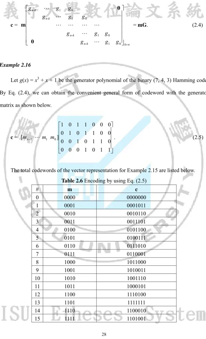
(41) = m(x)g(x) = 1(x3 + x + 1) = x3 + x + 1. The total 16 codewords are listed below. Table 2.5 Encoding by c(x) = m(x)g(x) #. m(x). 0. 0. c(x) 0 3. 1. 1. x +x+1. 2. x. x4 + x2 + x. 3. x+1. x4 + x3 + x2 + 1. 4. x2. x5 + x3 + x2. 5. x2 + 1. x5 + x2 + x + 1. 6. x2 + x. x5 + x4 + x3 + x. 7. x2+ x + 1. x5 + x4 + 1. 8. x3. x6 + x4 + x3. 9. x3 + 1. x6 + x4 + x + 1. 10. x3 + x. x6 + x3 + x2 + x. 11. x3 + x +1. x6 + x2 + 1. 12. x3 + x2. x6 + x5 + x4 + x2. 13. x3 + x2 + 1. x6 + x5 + x4 + x3 + x2 + x + 1. 14. x3 + x2 + x. x6 + x5 + x. 15. x3 + x2 + x + 1. x6 + x5 + x3 + 1. The polynomial multiplication in Eq. (2.2) can be reexpressed below by using matrix multiplication.. c(x) = m(x)g(x) = (mk-1x k-1 + … + m1x + m0)g(x) = mk-1x k-1g(x) + … + m1xg(x) + m0g(x). = [mk 1. (2.3).  x k 1 g ( x)    .   m1 m0 ]  xg ( x)     g ( x) . Eq. (2.3) provides a convenient general form of codeword with generator matrix for cyclic codes.. 27.

(42)  g n-k    m c=    0.  g n-k. g1  . g0 g1  g n-k. g0 . .  g n-k. g1 g 0  g1. 0    = mG.   g 0  k n. (2.4). Example 2.16. Let g(x) = x3 + x + 1 be the generator polynomial of the binary (7, 4, 3) Hamming code. By Eq. (2.4), we can obtain the convenient general form of codeword with the generator matrix as shown below.. c = [mk 1. 1 0  m1 m0 ] 0  0. 0 1 0 0. 1 0 1 0. 1 1 0 1. 0 1 1 0. 0 0 1 1. 0 0 . 0  1. (2.5). The total codewords of the vector representation for Example 2.15 are listed below. Table 2.6 Encoding by using Eq. (2.5) # 0 1 2 3 4 5 6 7 8 9 10 11 12 13 14 15. m 0000 0001 0010 0011 0100 0101 0110 0111 1000 1001 1010 1011 1100 1101 1110 1111. c 0000000 0001011 0010110 0011101 0101100 0100111 0111010 0110001 1011000 1010011 1001110 1000101 1110100 1111111 1100010 1101001 28.

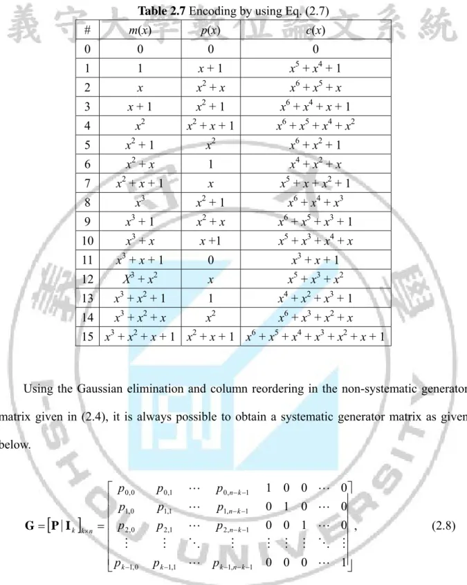
(43) The encoding method described above is called non-systematic encoding because the original message does not appear in the codeword. Linear codes may be systematic or non-systematic. For a systematic linear code, the original message appears unaltered in the. codeword. In a systematic code, every codeword consists of the original k message digits along with n – k additional parity check digits. Retrieving the original k message bits from the codeword is trivial in a systematic code. Non-systematic codes have codewords that bare no resemblance to the original unencoded information. Building good linear codes and designing efficient decoding algorithms forms the basis for most of the work in error control codes. Systematic codes are often preferred over the non-systematic codes because they allow quick look. The parity check digits of a systematic code can be obtained by parity check polynomial p(x) = m(x)xn-k mod g(x).. (2.6). Thus, the representation of the systematic codeword with parity check digits in the higher n – k positions is shown below.. c(x)= xk(m(x)xn-k mod g(x)) + m(x).. (2.7). Example 2.17. By using Eq. (2.7), the total 16 codewords of systematic (7, 4, 3) Hamming code are listed in Table 2.7.. 29.

(44) Table 2.7 Encoding by using Eq. (2.7) #. m(x). p(x). 0. 0. 0. c(x) 0 5. 1. 1. x+1. x + x4 + 1. 2. x. x2 + x. x6 + x5 + x. 3. x+1. x2 + 1. x6 + x4 + x + 1. 4. x2. x2 + x + 1. x6 + x5 + x4 + x2. 5. x2 + 1. x2. x6 + x2 + 1. 6. x2 + x. 1. x4 + x2 + x. 7. x2 + x + 1. x. x5 + x + x2 + 1. 8. x3. x2 + 1. x6 + x4 + x3. 9. x3 + 1. x2 + x. x6 + x5 + x3 + 1. 10. x3 + x. x +1. x5 + x3 + x4 + x. 11. x3 + x + 1. 0. x3 + x + 1. 12. X3 + x2. x. x5 + x3 + x2. 13. x3 + x2 + 1. 1. x4 + x2 + x3 + 1. 14. x3 + x2 + x. x2. x6 + x3 + x2 + x. 15 x3 + x2 + x + 1 x2 + x + 1 x6 + x5 + x4 + x3 + x2 + x + 1. Using the Gaussian elimination and column reordering in the non-systematic generator matrix given in (2.4), it is always possible to obtain a systematic generator matrix as given below.. G  P∣I k k n.  p 0, 0  p  1,0   p 2,0     p k 1, 0 . p 0,1 p1,1.  . p 0,n  k 1 p1,n  k 1. p 2,1.   . p 2,n  k 1.  p k 1,1.  p k 1,n  k 1. 1 0 0  0 0 1 0  0 0 0 1  0 ,       0 0 0  1. (2.8). where Ik is the k  k identity matrix and P is the matrix of size k  (n – k). The codeword c can be obtained from. c  mG.  [mk 1  m1 m0 ]P∣I k . .. (2.9).  [c n 1  c k 1 c k mk 1  m1 m0 ] 30.

(45) Example 2.18. Using the Gaussian elimination and column reordering in the non-systematic generator matrix given in Eq. (2.5), Eq. (2.8) can be rewritten as 1 0 G 1  1. 1 0 1 0 0 0 1 1 0 1 0 0 . 1 1 0 0 1 0  0 1 0 0 0 1. (2.10). Using Eq. (2.10), the total 16 codewords of systematic (7, 4, 3) Hamming code are listed in Table 2.8. Table 2.8 Encoding by using Eq. (2.10) #. m. c. 0. 0000. 0000000. 1. 0001. 1010001. 2. 0010. 1110010. 3. 0011. 0100011. 4. 0100. 0110100. 5. 0101. 1100101. 6. 0110. 1000110. 7. 0111. 0010111. 8. 1000. 1101000. 9. 1001. 0111001. 10. 1010. 0011010. 11. 1011. 1001011. 12. 1100. 1011100. 13. 1101. 0001101. 14. 1110. 0101110. 15. 1111. 1111111. 31.

(46) 2.4 The Basic Properties of QR Codes Let (n, (n + 1) / 2, d) denote a binary QR code with generator polynomial g(x) over a ground field GF(2) and let n be a prime number of the form n = 8l ± 1, where l is an arbitrary positive integer and m be the smallest positive integer such that n divides 2m – 1. The set Qn of quadratic residues modulo n is the set of nonzero squares modulo n; that is, Qn  { j j  x 2 mod n for 1  x  n  1}.. (2.11). Let m be the smallest positive integer such that n divides 2m – 1 and let  be a generator of the multiplicative group of all nonzero elements in GF(2m). Then the element  = u in. GF(2m), where u = (2m – 1)/n, is a primitive n-th root of unity in GF(2m). A binary (n, k, d) QR code is a cyclic code with the generator polynomial g(x) of the form, g ( x)   ( x   i ) .. (2.12). iQn. A codeword of the (n, k, d) QR code is a binary vector c = (cn-1,…, c1, c0) so that its associated polynomial c(x) = cn-1x n-1 + … + c1x + c0 is a multiple of g(x). If the codeword c is transmitted through a noisy channel, and if the vector r = (rn-1,…, r1, r0) is received, then the polynomial r(x) = rn-1x n-1 + … + r1x + r0 corresponding to r can be expressed as a sum of the code polynomial c(x) and the error (or error pattern) polynomial e(x) = en-1x n-1 + … + e1x + e0, namely r(x) = c(x) + e(x). The set of known syndromes is obtained by evaluating r(x) at the roots of g(x), i.e.,. 32.

(47) S i  r ( β i )  c ( β i )  e( β i )  e( β i ) n 1.  ej (βi ) j. .. (2.13). j 0 v.   Z ij , i  Qn j 1. The following lemma given in [16] shows that the mapping between the syndromes and error patterns is one-to-one. For a detailed proof, see [16].. Lemma 2.1 For a (n, k, d) binary cyclic code with the error-correcting capability. t  (d  1) / 2 , the mapping between the syndromes of a code and the error patterns e of weight ≤ t is one-to-one. If, during the data transmission, v errors occur in the received vector r, then the error polynomial has v nonzero terms, namely, e( x)  x l1    x lv , where 0  l1 <…< lv  n–1. And the syndrome S i can be written as S i  Z 1i    Z vi , where i  Qn and Z j  . lj. for. all 1  j  v, are called the error locators. Expanding Eq. (2.13), we obtain the following a sequence of 2t algebraic syndrome equations in the v unknown error locations. S1  Z 1  Z 2    Z v S 2  Z 12  Z 22    Z v2 S 3  Z 13  Z 23    Z v3. .. (2.14).  S 2t  Z 12t  Z 22t    Z v2t Eq. (2.14) is called Power-sum symmetric functions. Since they form s system of nonlinear algebraic equations in multiple variables, they are somewhat difficult to solve in a direct manner. For any binary QR codes, there is an obvious relation among syndromes, namely S 2i  S i2 , with sub-index modulo n if necessary. Assume that v errors occur: One. 33.

(48) defines the error-locator polynomial L(x) to be the polynomial of degree v v. v. j 1. j 1. L( x)   ( x  Z j )  x v   σ j x v  j ,. (2.15). where the coefficients of L(x) are v. σ1   Z i  Z1    Z v i 1. σ 2   Z i Z j  Z 1 Z 2  Z 1 Z 3    Z v 1 Z v i j. .. (2.16).  v. σ v   Z i  Z 1 Z 2  Z v 1 Z v i 1. The expressions in Eq. (2.16) are the elementary symmetric functions of the error locators. In order to develop the algebraic decoding algorithm, it is well known that the power sums Si and the elementary symmetric functions σj are related by the following Newton identities. For the detailed proof, see [2].. Theorem 2.10 (The Newton identities) For a binary QR code, there is a unique set of identities between the power sums Si and the elementary symmetric functions σj given in the following: i 1. S i   σ j S i  j  σ j  0 (1  i  v, i  odd ), j 1. i 1. S i   σ j S i  j  0 (1  i  v, i  even ),. (2.17). j 1 v. S i   σ j S i  j  0 (i  v ). j 1. If there is a sufficient number of consecutive known syndromes for a given number of errors, one can directly solve from Newton’s identities for σj, 1 ≤ j ≤ v. However, if there are not enough consecutive syndromes, one first tries to find the unknown syndromes, and then to. 34.

(49) find L(z) from the Newton identities. In either case, once L(z) is found, the error pattern is found by a Chien search method of the roots of L(z) over the set of all the n-th roots of unity. Finally, the error location numbers are the reciprocals of these roots. The parameters of binary QR codes with code length less than or equal to 241 are listed in Table 2.9. n. k. Table 2.9 The parameters of some binary QR codes d n k d n. 7 17 23 31 41 47 71 73. 4 9 12 16 21 24 36 37. 3 5 7 7 9 11 11 13. 79 89 97 103 113 127 137 151. 40 45 49 52 57 64 69 76. 35. 15 17 15 19 15 19 21 19. 167 191 193 199 223 233 239 241. k. d. 84 96 97 100 112 117 120 121. 23  27  27  31  31  25  31  31.

(50) Chapter 3 Algebraic Decoding Algorithm of the Binary Systematic (23, 12, 7) Golay Code 3.1 Background of the Binary Systematic (23, 12, 7) Golay Code To introduce the binary (23, 12, 7) Golay code, we first compute the set of quadratic residues, modulo 23, Q23 as follows: Q23  { j j  x 2 mod 23 for 1  x  22}. (3.1).  {1, 2, 3, 4, 6, 8, 9, 12, 13, 16, 18}.. Let  be a root of primitive polynomial p(x) = x11 + x2 + 1; that is, p() = 0 and m = 11. Obviously, an element  = u, where u = (2m – 1)/n = (211 – 1)/23 = 89, is a primitive 23-th root of unity in GF(211), and the power 11 is the smallest positive integer such that 23211–1. Let  be a primitive element in GF(211) such that  is a generator of the multiplicative group of 211–1 nonzero elements in GF(211). A binary (23, 12, 7) Golay code is a QR code or a cyclic code with the generator polynomial g(x) of the form. g ( x)  iQ ( x  β i )  x11  x 9  x 7  x 6  x 5  x  1, 23. (3.2). where the degree of g(x) is 11. Since  is a primitive root of g(x) and is also an element of order 23 in GF(211),  can be generated the cyclic subgroup of 23 elements, G 23  (1,  ,  2 ,  ,  22 ) in the multiplicative group of GF(211) by a use of Eq. (3.2). The (23, 12, 7) Golay code generated by g(x) in this manner is a perfect code in a sense that the codewords and their three error correction spheres. 36.

(51) exhaust the vector space of 23-bit binary vectors. Because the minimum distance of this code is d = 7, the inequality 2v + 1 ≤ 7 is valid, where v is the actual number of errors to be corrected. Hence, the (23, 12, 7) Golay code allows for the correction of up to t  (d  1) / 2  3 errors, where x  denotes the greatest integer less than or equal to x. From Section 2.5.1, we know that a binary vector c = (c22,…, c1, c0) is a codeword if and only if its associated polynomial c(x) = c22x 22 + … + c1x + c0 is a multiple of g(x), where ci  GF(2). If r = (r22,…, r1, r0) is a received vector, then its associated polynomial r(x) = r22x 22 + … + r1x + r0 can be expressed as a sum of the transmitted code polynomial c(x) and the error polynomial e(x) = e22x 22+ … + e1x + e0; that is, r(x) = c(x) + e(x) or r = c + e. From Eq. (2.13), the set of known syndromes is obtained by evaluating r(x) at the roots of g(x); that is, S i  e(  i )  e 22 (  i ) 22    e1 (  i )  e0 ,. (3.3). where i  Q23. If v  t errors occur in the received vector, then the error polynomial has v nonzero terms, namely, e( x )  x r1  x r2  x r3    x rv , where 0  r1 < r2 <…< rv  22. For i  Q23, the i-th syndrome S i is given by Si  (  r1 )i  (  r2 )i    (  rv )i = Z1i  Z 2i    Z vi , where the error locators are Z j  . rj. for all 1  j  v.. For the (23, 12, 7) Golay code, one has the following equalities among the known 2. 4. 3. 5. 6. 7. syndromes: S 2  S12 , S 4  S12 , S8  S12 , S16  S12 , S9  S12 , S18  S12 , S13  S12 , 8. 9. 10. S3  S12 , S6  S12 , S12  S12 . Thus, all the known syndromes can be expressed as some i. powers of S1. Table 3.1 shows the values of indices ti if S ti  S 2j for the (47, 24, 11) QR code. The numbers in the leftmost column and the first row indicate the indices j’s and i’s, respectively.. 37.

(52) Table 3.1 The values of indices S ti  S 2j. i. j 1. i. 0. 1. 2. 3. 4. 5. 6. 7. 8. 9. 10. 1. 2. 4. 8. 16. 9. 18. 13. 3. 6. 12. 3.2 Algebraic Decoding Algorithm Developed by Elia In ADA, the most important work for decoding the (23, 12, 7) QR code is to compute the unknown syndrome S5. Elia [7] developed an ingenious method to avoid the computation of. S5. Since  is a root of g(x),  3, and  9 are also roots of g(x). By using these roots, we can compute three syndromes as follows:. S1 = r()= e(), S3 = r( 3) = e( 3), and S9 = r( 9) = e( 9),. (3.4). where S1, S3, and S9 are called the known syndromes of this code. From Eq. (2.15), we have the following error-locator polynomial 3. 3. j 1. j 1. L ( x )   ( x  Z j )  x 3   σ j x 3 j  x 3  σ 1 x 2  σ 2 x  σ 3 ,. (3.5). where σ1 = Zl + Z2 + Z3, σ2 = ZlZ2 + Z2Z3 + Z3Z1, σ3 = ZlZ2Z3. Observe that S13  S 3 . Let. . a,b. denote the sum of all six terms of the type Z ia Z bj , i, j.  {1, 2, 3}, and set S a  Z 1a  Z 2a  Z 3a . Then S 9  S19  1,8  σ 2 S 7  σ 3 S 32. (3.6). S 7  S1 S 32  1, 6  σ 2 S 5  σ 3 S14. (3.7). S 5  S15  1, 4  σ 2 S 3  σ 3 S12 .. (3.8). 38.

(53) Furthermore, σ 3  S 3  σ 2 S1  S13 .. (3.9). Combining these, we find D ( S13  S 3 ) 2  ( S19  S 9 ) ( S13  S 3 )  (σ 2  S12 ) 3 .. (3.10). From (3.9) and (3.10) we have σ 2  S12  D 1 / 3 and σ 3  S 3  S1 D 1 / 3 .. (3.11). Of course, σ 1  S1 by definition. Note that σ 3  0 if two errors have occurred. The cube root D1/3 is in GF(211), and it can be computed as a power of exponent 1365, i.e., D1/3 =. D1365. Finally, once L(x) is known we can use the Chien search [5] to find the error locations. Elia’s algorithm for decoding the (23, 12, 7) Golay code is summarized as below. 0, no errors if S1 = 0.. x + S1, one error if S13  S 3 and S19  S 9 . L(x) =. x 2  S1 x  ( S12 . S3 ) , two errors if S1 D1 / 3  S 3 . S1. (3.12). x 3  S1 x 2  (S12  D1 / 3 ) x  (S 3  S1 D1 / 3 ) ; otherwise, 3 errors.. 3.3 The Decoding of the Binary (24, 12, 8) Golay Code A binary (24, 12, 8) Golay code can be formed by adding an overall parity-check bit to the (23, 12, 7) Golay code. The following extension of decoding algorithm for the (24, 12, 8) Golay code can be used to correct three errors and detect four errors. To illustrate this, let r denote the received word as expressed as the binary form without its overall parity bit p. It is convenient also to let the symbol P denote the decoding procedure of the (23, 12, 7) code. The. 39.

(54) decoding scheme of the code augmented by a parity bit given in [17] is summarized in the following: i) If there are v ≤ t – 1 = 3 – 1 = 2 errors occurred in the received word r, then it can be decoded by P regardless of the value of the overall parity bit. ii) If there are more than 2 errors occurred in the received word, then after using P to decode r, the parity p’ is recomputed and then compared with the received parity p. If. p’  p, four errors are detected from the decoder.. 3.4 A Fast Method for Computing the Multiplication and Inverse in GF(2m) The computation of the inverse and multiplication is very complicated in the Finite field. The following theorem given in [37] provides a very fast method to reduce the computational complexity in the Finite field. Thus, the decoding time can be significantly reduced.. Theorem 3.1 Let (n, k, d) be a binary QR code over GF(2) and let α be a primitive root of m. unity in GF(2m) such that α 2  α . If an element   GF(2m), then the inverse of  in GF(2m) has  -1   2. m. 2. . Let 2m – 2 be decomposed as 21 + 22 + 23 +…+ 2m-1, then -1 can be. expressed as. -1 =  2. 1.  2 2  2 3  2 m 1. 1. 2. 3. =  2  2  2  2. m 1. .. (3.13). For example, for the binary (23, 12, 7) Golay code, the inverse of an element   GF(211) is -1 = 2. m-2. = 2. 11-2. = 2046. However, the power of  is very large, thereby increasing the. computational complexity. Next, also by using Theorem 3.1, the power 2046 be first. 40.

(55) decomposed as the binary representation 21 + 22 +…+ 210, then -1 can be expressed as -1 =. 2. D1 6(2. 1. 1.  2 2  2 3   210. =. 1. 2. 3.  2  2  2  2. )  6 ( 2 2 )  4 ( 2 3 )  3( 2 4 )  3( 2 5 )  2 ( 2 6 )  2 ( 2 7 )  2 8  2 9. 10. .. D1/3. Moreover, 1. 2. =. D1365. =. 9. = D1 D 6 ( 2 ) D 6 ( 2 )  D 2 . Thus, the power of the. syndromes can easily be accomplished by using successive squaring operations and multipliers. Such a fast computational method can efficiently reduce the computer execution time up to hundreds of times when the power of the syndrome is very large. Therefore, the improved ADA is considerably faster in decoding time than that of the method given in [7].. 41.

(56) Chapter 4 Syndrome-Weight Decoding Algorithm of the Binary Systematic (23, 12, 7) Golay Code The syndrome decoder [5] is a very efficient method of decoding a linear code over a noisy channel. In essence, the syndrome decoder is a minimum distance decoding using the syndrome together with the corresponding error pattern (syndrome-error pattern) lookup table. Due to the linearity of the code, a binary (n, k, d) QR code with minimum distance d is capable of correcting up to t errors, where t  (d  1) / 2 . The full size of the syndromes-error pattern lookup table is Rn  i 1 t. code, R23 =.    3. 23 i 1 i.   . Therefore, for the (23, 12, 7) Golay n i. = 2047, and thus this table is called the full lookup table (FLT). Each. syndrome and error pattern needs 2 and 3 bytes, respectively, to store in the memory. Thus, the total memory size for the FLT is (2047  (2 + 3)) / 1024 ≒ 10 kbytes. However, such a large memory is somewhat less efficient in practice. For this reason, searching a syndrome in this large table requires highly computational complexity. In this chapter, the reduction of the memory requirement of the proposed algorithm is considered.. 4.1 Syndrome Decoder with a Reduced-Size Lookup Table To reduce the memory requirement, the well-known syndrome decoder with a RSLT [5, p118] is used. The syndrome decoder with a RSLT is a very efficient method of decoding linear cyclic codes over a noisy channel for moderate code lengths. In essence, the syndrome. 42.

(57) decoder is a minimum distance decoding using the syndromes corresponding to their error patterns in the lookup table. Due to the property of cyclic code, it allows for the lookup table to be reduced in memory size. In order to illustrate the syndrome decoder with a RSLT, the following theorem is needed. For a detailed proof, see [5, p118].. Theorem 4.1 Let s(x) be the syndrome polynomial corresponding to a received polynomial. r(x). Also, let r(1)(x) be the polynomial obtained by cyclically shifting the coefficients of r(x) one bit to the right. Then the remainder obtained when dividing xs(x) by g(x) is the syndrome. s(1)(x) corresponding to r(1)(x).. Definition 4.1 Using Theorem 4.1, if n is prime, then the number of the syndromes and error patterns of the syndrome decoder needs 1/n of the size of FLT, namely Rn / n . If n is not prime, then the number of the syndromes and error patterns of the syndrome decoder only needs Rn / n  , where x  denotes the least integer large than or equal to x. This reduced table is called the reduced-size lookup table (RSLT)..  3  For (15, 5, 7) cyclic code, the RSLT has R15 / 15 =  15 i  / 15 = 39 elements.  i 1  Therefore, the required memory size of the RSLT is 39  (2 + 2) = 156 bytes. For (23, 12, 7).   / 23 = 2047/23 = 89 elements. Therefore, the 3. Golay code, the RSLT has R23 / 23 =. i 1. 23 i. required memory size of the RSLT is 89  (2 + 3) = 445 bytes. For (31, 16, 7) QR code, the.   / 31 = 4491/31 = 161 elements. Therefore, the required memory 3. RSLT has R31 / 31 =. i 1. 31 i. size of the RSLT is 161  (2 + 4) = 966 bytes. For these codes, the relationship of the syndromes and their corresponding error patterns in the RSLT is shown in Appendix A. 43.

(58) For the binary systematic (23, 12, 7) Golay code, it follows from (2.8) that the k  n generator matrix G can be expressed as follows:. G  P∣I 12 1223.  p0, 0 p  1, 0   p 2, 0     p11,0 . p 0,1 p1,1 p 2,1  p11,1.  p0,10  p1,10  p 2,10    p11,10. 1 0 0  0. 0 1 0  0. 0 0 1  0.     . 0 0 0 ,   1 1223. (4.1). where Ik is the k  k = 12  12 identity matrix and P is the matrix of size k  (n – k) = 12  11 given by 1 1  1  1 1  0 P   0  1 0  0  1 0. 0 1 0 1 1 1 0 0 0 1 1 1 1 1 0 0 1 0 0 1 1 0 1 0 0 1 0 1 0 1  1 0 0 0 1 1 1 0 1 1 1 0 0 1 1 0 1 1 0 0  1 1 0 0 1 1 0 1 1 0 .  0 1 1 0 0 1 1 0 1 1  0 1 1 0 1 1 1 1 0 0 1 0 1 1 0 1 1 1 1 0  0 1 0 1 1 0 1 1 1 1  0 1 1 1 0 0 0 1 1 0 1 0 1 1 1 0 0 0 1 1 1211. (4.2). From Eq. (2.9), namely c = mG, one can obtain the systematic codeword.. Example 4.1. For the binary systematic (23, 12, 7) Golay code, assume that the message vector is m = (000000000001). Using Eq. (2.9) and Eq. (4.2), one obtains the codeword c = (01011100011000000000001).. The systematic parity check matrix H of size (n – k)  n = 23  47 can be expressed as. 44.

(59) follows:. . H  I nk | P T. . ( n-k ) n. 1 0   0   0 . 0 0  0 1 0  0. p0, 0 p 0,1. p1, 0 p1,1.  . 0 1  0. p0, 2. p1, 2. . . . . .   . 0 0  1. p 0,10. p1,10 . p11, 0  p11,1  p11, 2  ,    p11,10  1123. (4.3). where PT is a (n – k)  k = 11  12 transpose matrix of P and In-k is a (n – k)  (n – k) = 11  11 identity matrix. The vector form of syndrome can be defined by 1 0  s = rHT = (r22 , , r0 , r1 ) 0   0 . 0 0  0 1 0  0 0 1  0. p 0,0. p1, 0. . p 0,1. p1,1. . p1, 2 . .   . p 0, 2 . 0 0  1. p 0,10. p1,10 . . . T. p11, 0  p11,1  p11, 2  ,    p11,10 . (4.4). I  . where the HT denotes a n  (n – k) = 23  11 transpose matrix of H; that is, H T   11   P  2311 The syndrome decoder only needs to compute the syndrome of r for every received word, find the corresponding error pattern, and correct r. Thus, the computation of the error-locator polynomial L(z) needed in the ADA can be completely avoided. This is the reason why the syndrome decoder significantly reduces the computational complexity. If r occurs with no error, then the syndrome s = rHT = (c + 0)HT = cHT = 0, where 0 denotes a zero vector; otherwise, s = rHT = (c + e)HT = 0 + eHT = eHT.. Example 4.2. The codeword c is given in the Example 4.1. Assume that the error pattern is e = (00000000000000000000000000000000000000000000110), then the received word is r = c +. e = (11101110110111000110001000000000000000000000111) and the syndrome is s = rHT = (10111111011). 45.