一個關於先進製程技術關鍵區域分析工具之實作

國

國

國

立

立

立 交

交

交 通

通

通

大

大

大

學

學

學

電 機

_{學 院IC設 計 產 業 研 發 碩 士 班}

碩

碩

_{碩 士}

_士

_{士 論}

論

論 文

文

文

一個關於先進製程技術關鍵區域分析工具之實作

An Implementation of More Efficient Critical Area Analyzer for

Advanced Manufacturing Technology

研

_{究 生： 陳柏州}

指導教授： 陳宏明 博士

一個關於先進製程技術關鍵區域分析工具之實作

An Implementation of More Efficient Critical Area Analyzer for

Advanced Manufacturing Technology

研

_{究 生 ： 陳柏州}

_{Student: Bo-Zhou Chen}

指 導 教 授 ： 陳宏明 博士

Advisor: Prof. Hung-Ming Chen

國

立 交 通 大

學

電 機

_{學 院IC設 計 產 業 研 發 碩 士 班}

碩 士 論 文

A Thesis

Submitted to College of Electrical and Computer Engineering

National Chiao Tung University

in Partial Fulfillment of the Requirements

for the Degree of

Master

in

Industrial Technology R & D Master Program on IC Design

August 2008

Hsinchu, Taiwan, Republic of China

一個關於先進製程技術關鍵區域分析工具之實作

學生： 陳柏州

指 導 教 授 ： 陳宏明 博士

國立交通大

_{學電機學院產業研發碩士班}

摘

要

An Implementation of More Efficient Critical Area Analyzer for

Advanced Manufacturing Technology

Student: Bo-Zhou Chen

Advisor: Prof. Hung-Ming Chen

Industrial Technology R & D Master Program of

National Chiao Tung University

ABSTRACT

In this thesis, we present a method of computing critical area for short faults of an integrated circuit from the mask layout. The method is based on the concept of sampling framework and the geometry computation of critical area. By constructing the density table of layout, our weighted sampling approach can be more accurate and more suitable for the larger device. The algorithm has been implemented within OpenAccess platform to allow efficient extraction of the critical area from an arbitrary mask layout. The results show that this method can reduce computation cost; meanwhile, it can maintain the accuracy.

誌

誌

誌

謝

謝

謝

目

目

目

錄

錄

錄

2.1 Critical Area and Yield Models . . . 3

2.2 Previous Works . . . 5

2.2.1 Geometric Method . . . 5

2.2.2 Monte Carlo Method . . . 6

2.2.3 Stochastic Method . . . 7

2.4 Problem Formulation . . . 9

3 Algorithm . . . 10

3.1 Data Translation and Transformation . . . 10

3.2 Density Table Generation . . . 14

3.3 Sampling Framework . . . 15

3.3.1 Weighted Sampling . . . 15

3.3.2 Shape Expansion . . . 17

3.3.3 Polygon Clipping . . . 17

3.4 Critical Area Estimation . . . 21

4 Experimental Results . . . 23

5 Conclusions and Future Works . . . 26

參考文獻 . . . 27

表

表

表

目

目

目

錄

錄

錄

2.1 Yield model table . . . 4

3.1 Mapping table . . . 12

圖

圖

圖

目

目

目

錄

錄

錄

1.1 The definition of critical area. . . 2

2.1 CAA and yield prediciton workflow [2]. . . 4

2.2 An example for geometric methods : We can obtain the actual critical area by the geometric method, but the computational cost is expensive. . . 5

2.3 An example for monte carlo simulation : The more defects are sprinkled, the more accurate critical area will be obtained. . . 6

2.4 The OpenAccess support across flow [1] . . . 7

2.5 The OpenAccess modularization [1] : The conceptual modularization is re-flected in top-level header includes, link libraries, and required initialization calls. . . 8

3.1 The flow of our algorithm. . . 11

3.2 Translation [1] : Offset value of x and y. . . 13

3.3 The example for density table. . . 14

3.4 Region query flow of execution [1]: Taking oaShape as an example, show a code tracing using plug-in. . . 15

3.5 Shape expansion algorithm. . . 18

3.6 The examples for short failure by shape expansion : two different defect size. . . 18

3.7 The valid sample region : The shape of polygons inside sample region is valid. . . 19

3.8 The polygon clipping algorithm – Weiler-Atherton. . . 20

3.9 The example by Weiler-Athertion algorithm. . . 20

3.10 The example by sweep-line algorithm : scan-line from left to right. . . 21

3.11 Orthogonal segment sweep line algorithm. . . 22

4.1 The comparsion of single shape-expan and the different density table. . . 23

4.2 The comparsion of single sample region size and the two tpye sample region size. . . 25

第

第

_{第 1 章}

章

章

_Introduction

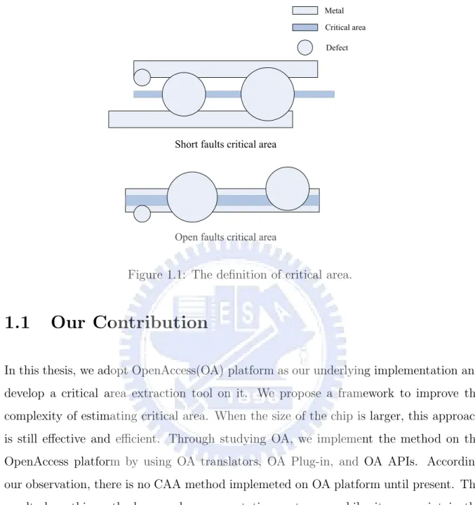
With the advancement of the deep sub-micron (DSM) VLSI design, the yield is becom-ing an urgent problem. With all aspects of the nano-era IC manufacturbecom-ing, yield has been traditionally limited only by defect density but now it is influenced greatly by the interaction of design elements and variation of the manufacturing. It means that many random defects will cause the loss of yield during the lithography on the manufacturing process. We usually used the rule-based style to predict the yield in the past, but it will not reflect the effect of process variation. Currently the model-based method is intro-duced for prediction and it can reflect the sensitivity of the random defects to the yield more accurately, thus we have adopted this concept in our critical area extraction, the definition of critical area is shown in Figure 1.1.

First, we show that why we need to compute critical area in the layout. The oc-currence of random defects is due to the contamination or particles sprinkled from the process equipments. These random defects will eventually cause a catastrophic functional failure which is an open or a short. Critical area is the region where random defects cause circuit failures. Based on the failure type(open or short) caused by random defects, they can be classified into two types “extra material” defect causing short faults,and “missing material ” defect causing open faults. Reducing yield loss is not only the foundries’ responsibility but also relies on the designer’s work. Therefore, critical area is a key layout attribute that can be measured a design’s sensitivity to the loss of yield [3], and it is treated as a yield metric. In the design, critical area can be defined as the area in the design where the circuit failures are most likely to occur, which is the region where the center of the particle must fall to create a short or open circuit, as shown in Figure 1.1.

Critical area provides an accurate metric for yield prediction. The need of implemen-tion tools that incorporate critical area analysis is necessary for improving the predicimplemen-tion of the yield. We are motivated to develop critical area analysis (CAA) technique by the fact that it is crucial to find the critical area (or minimize it) for yield improvement.

Metal Critical area Defect

Figure 1.1: The definition of critical area.

1.1

Our Contribution

In this thesis, we adopt OpenAccess(OA) platform as our underlying implementation and develop a critical area extraction tool on it. We propose a framework to improve the complexity of estimating critical area. When the size of the chip is larger, this approach is still effective and efficient. Through studying OA, we implement the method on the OpenAccess platform by using OA translators, OA Plug-in, and OA APIs. According our observation, there is no CAA method implemeted on OA platform until present. The result show this method can reduce computation cost; meanwhile, it can maintain the accuracy.

1.2

Thesis Organization

This thesis is organized as follows. Chapter 2 reviews some previous works and basic concepts of critical area. Chapter 3 presents the flow of this work and the algorithm we implement. Chapter 4 gives experimental results. We conclude our work in Chapter 5.

第

第

_{第 2 章}

章

章

_Preliminary

In this chapter, we first discuss the relations between critical area and yield models. Second, we will introduce previous works about the methods of critical area extaction. By these methods, we realize how to implement the critical area extraction in those previous works. Then we will describle the OpenAccess platform. A brief introduction about the goals and the advantages of OpenAccess will be presented. Last, we will give our problem formulation of this thesis.

2.1

Critical Area and Yield Models

When evaluating the yield, the defect size distribution and the critical area are essential . Generally, the defect size distribution is defined as 1/xp _{by experience, where x is the}

defect size and p is typically in the range of 2 and 3.5. More specifically [4], the defect size distribution function is the density function of the defect size. It is defined as follows : s(x) =    cx−q−1 0 xq, 0 ≤ x ≤ x0 cxp−10 x−p, x0 ≤x ≤ ∞ p 6= 1, q > 0, c = (q + 1)(p − 1)/(q + p)

Let Ac(x) be a critical area of defect size x. The average critical area Ac is defined as the

following equation :

Ac =

Z _∞

0

Ac(x)s(x)dx

The average defect density of all sizes is called D0 and average defect density of size x is

called D(x), the relationship between them is defined as :

D(x) = D0s(x)

Therefore, the average number u of faults caused by defects is defined as :

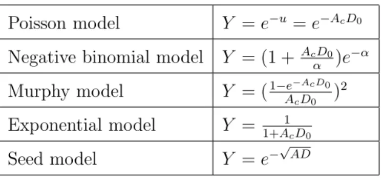
There are many different yield models proposed in the literature, which model should be used depends on the process versus die size. Table 2.1 shows some usual yield models.

Table 2.1: Yield model table

Poisson model Y = e−u _{= e}−AcD0

Negative binomial model Y = (1 + AcD0

α )e−α

Murphy model Y = (1−e−AcD0

AcD0 ) 2 Exponential model Y = 1 1+AcD0 Seed model Y = e− √ AD

Figure 2.1 shows the entire design flow and illustrates the relationship between CAA and yield prediction in the design flow. From Figure 2.1 we know that critical area and defect density are both essential when predicting the yield. However, the defect density is generally provided by the foundry. In other words, the accuracy of extracting critical area has great influence on the yield prediction.

2.2

Previous Works

Generally speaking, the methods of critical area extraction can be categorized by the following methods: geometric method, Monte Carlo mehtod, stochastic method.

2.2.1

Geometric Method

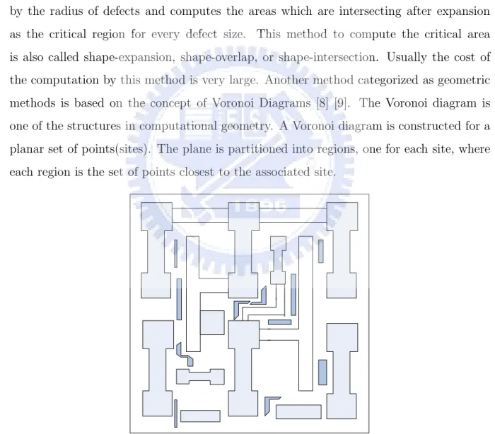
This method is based on the computational geometry [5] [6] [7]. It expands all polygons by the radius of defects and computes the areas which are intersecting after expansion as the critical region for every defect size. This method to compute the critical area is also called shape-expansion, shape-overlap, or shape-intersection. Usually the cost of the computation by this method is very large. Another method categorized as geometric methods is based on the concept of Voronoi Diagrams [8] [9]. The Voronoi diagram is one of the structures in computational geometry. A Voronoi diagram is constructed for a planar set of points(sites). The plane is partitioned into regions, one for each site, where each region is the set of points closest to the associated site.

Figure 2.2: An example for geometric methods : We can obtain the actual critical area by the geometric method, but the computational cost is expensive.

2.2.2

Monte Carlo Method

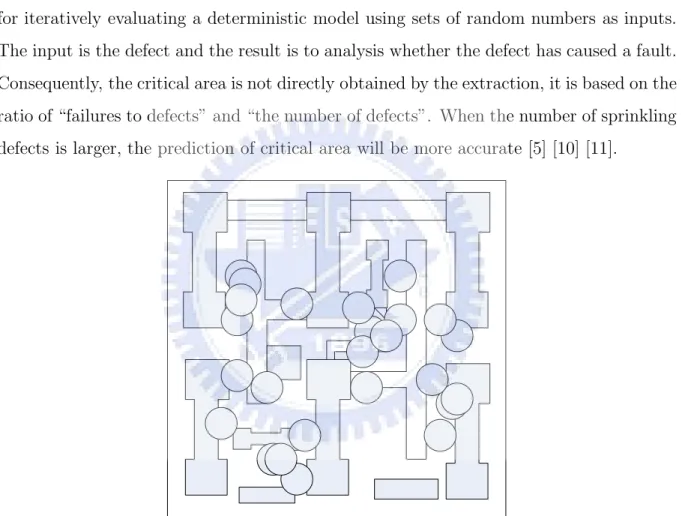
The method is also called “dot throwing” which was one of the methods used to find out the sensitivity of the layout to random defects. Taking the extra material defects as an example( shown in Figure 2.3 ), the implementation is to sprinkle a large number of defects with their radii distributed and they are randomly placed on the circuit layout, then check for each defect if it causes a failure. Monte Carlo simulation is a method for iteratively evaluating a deterministic model using sets of random numbers as inputs. The input is the defect and the result is to analysis whether the defect has caused a fault. Consequently, the critical area is not directly obtained by the extraction, it is based on the ratio of “failures to defects” and “the number of defects”. When the number of sprinkling defects is larger, the prediction of critical area will be more accurate [5] [10] [11].

Figure 2.3: An example for monte carlo simulation : The more defects are sprinkled, the more accurate critical area will be obtained.

2.2.3

Stochastic Method

With the complexity of design is growing, the computation cost of critical area extraction becomes large. Therefore, the sampling framework or analytical model [12] is adopted to estimate the critical area. One of the biggest advantage of the stochastic mehods is that it can extremely decrease the cost of the computation. Thus this method will be very useful for larger designs when this method can obtain good quality result within an acceptable degree. In the [13], they propose a method which is combined sampling framework with the actual critical area extraction,such as shape-expansion. The hybrid method can be performed efficiently and maintain accuracy.

2.3

OpenAccess : Modern EDA Database Adoption

OpenAccess(OA) is an up-to-date EDA database designed to enable interoperability among IC design tools. [14] The framework contains an open standard data access in-terface (API) and Reference Implementation of that API as shown in Figure 2.4.

The OpenAccess data model can be used to represent designs from post-synthesis netlists to tape out. The implementation was contributed by Cadence Design Systems. Now, the OpenAccess Coalition, a group of over 30 companies including EDA vendor and the correlation of semiconductor business administer the change to the OpenAccess API. The Silicon Integration Initiative manages the OpenAccess effort [14].

OpenAccess provides advantages to design flows and EDA tool developers. Today, the various data formats such as Verilog, DEF, and GDSII are usually incomplete and the translation between different tools is very inefficient. OpenAccess can solve these problems because it provides much tighter integration and the data model which can be read by applications through API is more complete. It is much more efficient than these data formats which are translated individually. Another advantage of OpenAccess is the capabilities provided by the API for developers.

Figure 2.5: The OpenAccess modularization [1] : The conceptual modularization is re-flected in top-level header includes, link libraries, and required initialization calls.

OpenAccess is an object-oriented API written by C++, which is provided for public usage. The API can be applied to a large portion of EDA domain. It contains the geometric support, routing, floorplanning, placement information, parasitic effects and even the technology information. It also supports the plug-in of Reference Implemention. These utilities such as Region Query, Multiple Design Management(DM) have been tuned for improved performance and memory efficiency.

In addition, some EDA vendors such as Matrix One, MentorGraphics, Silicon Navigator have products which use OA 2.2. In this thesis, we use OA platform to develop our critical area extraction framework. We use OA translator to translate the data very efficiently. OA APIs and PlugIns Reference Implemention can also improve the tool performance and memory efficiency .

2.4

Problem Formulation

In the i-th layer of the GDSII file, there is a set of the metal wires with n elements – W1, W2, . . . Wn. We want to extract the critical area from this metal wire set. Given a

set of the defect sizes with m values – x1, x2, . . . xm, the critical area A(x1) is defined as

the region that the centers of the defects with the size x1 falling in the midst of the wire

set to create the short or open failures. Hence, the critical area with defect sizes m in the n-th layer are A(x1), A(x2), . . . A(xm) individually. Our problem formulation is then

described as follows :

Given a layout description in the GDSII file, we will translate this layout information into an OA database and analyze the critical area with different defect sizes. Finally, the curve of critical area presenting in A(x1), A(x2), . . . A(xm) in the i-th layer will be

第

第

_{第 3 章}

章

章

_Algorithm

The methods in Section 2.2 have been proposed to extract the critical area, however there remains some problems about accuracy and efficiency of the computation. In this thesis, We will consider these issues and improve them. Because the random defects are distributed over the chip randomly, the main concept of our method is to use sampling by the distribution of density. Based on the attribute, the sampling framework can reduce computation time and maintain the accuracy of critical area analysis in the meanwhile.

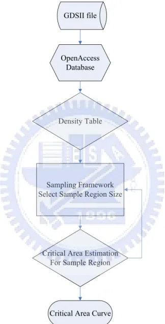
First, according to the critical area which is the most problematic area causing circuit failure, the density of layout will dominate this issue. If we obtain larger density in some region, the more potential failure will occur. We use the density table from one layer of the chip to illustrate this tendency. In order to reduce computation time, we attempt to divide the whole layout into a number of square grids and analyze the number of polygons in each grid. When we obtain the density table, we can determine the sample region and the number of sampling. Thus, the scale of the computation will descend from the entire layout to the local region. It means that it can decrease the quantity of computation. Next, we extract the critical area for sample regions respectively to estimate the critical area. According to previous works, the geometric methods are suitable for large layout, but the Monte Carlo methods are better for smaller layout. In our implementation, we will choose the shape-expansion method and sweep-line algorithm to implement critical area extraction. Finally, we can calculate the total critical area by summing up the critical area from each sample region. Because there are different defect sizes, each defect size has the corresponding critical area. The flow of our approach is shown in Figure 3.1.

3.1

Data Translation and Transformation

Since our method is implemented on OpenAccess platform, we have to translate the GDSII file into OA database. Then, we will introduce the functions of API adopting in

OpenAccess Database GDSII file

Density Table

Critical Area Estimation For Sample Region Sampling Framework Select Sample Region Size

Critical Area Curve

our algorithm. At first, the GDSII file is regarded as the input of our flow to translate the layout data into the OA database format. Consequently, we can access information from this OA database in the following steps of our flow. The command syntax of the translation is as follows [1]:

strm2oa -gds f ile -lib library [optional arguments]

• f ile is the GDSII file which will be translated.

• libray is the database name after translation.

• optional arguments is the user’s specific setup, here we use the default value.

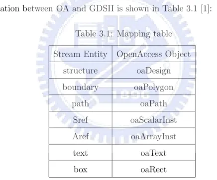
After executing this command, the OA database named as library will be produced. The mapping relation between OA and GDSII is shown in Table 3.1 [1]:

Table 3.1: Mapping table

Stream Entity OpenAccess Object structure oaDesign boundary oaPolygon path oaPath Sref oaScalarInst Aref oaArrayInst text oaText box oaRect

When the OA database is generated, the information needed for critical area ex-traciton is not ready yet, the translation only maps the data into OA database format. If we want to use the correct information, such as actual coordinates of the polygon, we have to execute some operations from other APIs. Due to the analysis of the critical area in one layer, we have to handle the information from the hierarchical structure into the flat structure. We will introduce OA API which we use the most during the translation. oaT ransf orm is the class implementing 2D Euclidean transformation, which includes two

parts : translation (Figure 3.2) and rotation direction (Table 3.2). Such as the follow-ing example, a constructor of oaTransform take an xof f set and yof f set value, and ”no ratation”.

oaTransform( oaInt4 xof f set, oaInt4 yof f set,oaOrient oacR0 );

• Translation – (X, Y) linear offsets

Figure 3.2: Translation [1] : Offset value of x and y.

• Orientation – angular rotation or mirror

Table 3.2: Orientation descriptions table [1]

oaOrientEnum Orientation Change oaOrientEnum Orientation Change oacR0 No change oacMX Mirror about X axis oacR90 Rotate 90◦ _{about origin oacMY Mirror about Y axis}

oacR180 Rotate 180◦ _{about origin oacMXR90 Mirror about X axis then rotate 90}◦

oacR270 Rotate 270◦ _{about origin oacMYR90 Mirror about Y axis then rotate 90}◦

From oaTransform, we can obtain the correct information about coordinates and translate them from hierarchical structure into flat structure.

3.2

Density Table Generation

The first step of our method is to construct a density table. A whole chip will be divided into n × n square grids on the specific layer and assigned a value(for each grid) which is the number of polygons appearing in this grid. An example of the density table is shown in Fgure 3.3.

Grid number

Polygons in this grid

Figure 3.3: The example for density table.

For example, grid 2 with a value 4, it describes that there are four polygons appear-ing in this grid and this value represents the degree of density in this area. Here, we called this value CountingNum. When the value is larger, it means that the density in this grid is denser. After building this table, we can obtain the layout

information about a whole chip, the distribution of the dense region and the sparse region. According to this density table and the characteristic of critical area, we can derive that the more crowded density is, the more critical areas we have. Hence, the density table can be regarded as a metric in the sampling framework(Section 3.3). Here we employ one OA API function to obtain the density table. The API function is a geometric analysis of a class called oaRegionQuery. oaRegionQuery is used to locate the geometric figures which might be touched, overlapped, or contained within a specified geometric rectangle. In OA, oaRegionQuery is a plug-in architecture. A default RegionQuery Plug-In, called “oaRQXY T ree”, is shipped with the Reference Implementation. The flow of execution is shown in Figure 3.4.

Figure 3.4: Region query flow of execution [1]: Taking oaShape as an example, show a code tracing using plug-in.

3.3

Sampling Framework

3.3.1

Weighted Sampling

The sampling strategy is based on random sampling, and the construction of the density table is built in the previous step. We will repeatedly do the random

sam-pling in the sample region until the value F calculated from the density table for each grid. The computation of the sampling value in each grid is shown as follows. The ratio that CountingNum is divided by the T otalCountingNum summed up by each grid is regarded as a weight, and it is multiplied by the total sample size. If the value is not an integer, we will round off. That is,

F = _{T otalCountingN um}CountingN um ×T otalSampleSize F : Sampling frequency of each grid

T otalCountingNum : sum up all CountingNum T otalSampleSize : the number of wanted sampling

Taking the Figure 3.3 as an example, the computing procedure is that CountingNum = 4, T otalCountingNum = 2 + 4 + 2 + 3 + 5 + 1 + 2 + 1 + 2 = 22, assumed the T otalSampleSize = 50, then F = (4/22) ∗ 50 = 9. It means that we will do ran-dom sampling 9 times in the grid 2. When executing ranran-dom sampling, we use a rectangle shape to extract the critical area in each action. We call it as a sample region. As shown in Figure 3.7, the setting of sample region has two constraints:

– Sample region size is smaller than the grid region size

– Sample region size is larger than the largest defect size

The reason in setting the rule 1 is that our purpose is for surveying sampling effects in this grid region. Therefore, the sample region size has to be smaller than this grid region size. In addition, for the rule 2, the sample region is used to estimate the critical area. The sample region size will affect the result. We find that when the sample region size is smaller than the largest defect size, it will cause the result inaccuracy. The explanation of this condition is related to the extraction method of critical area. The detail of this method will be discussed in the next section. When we use this extraction method, it will limit the sample region size in some range. Hence, the sample region size must be larger than the largest defect size, and it can ensure the accuracy of estimation. For the setting of total sample size, we adopt the

number of polygons appear in this layer multilied by a ratio as total sample size. This ratio is the number of CountingNum 6= 0 in n × n grids divided by n × n.

The selection of sample region size and total sample size has a great influence on the result. Both of them involve with the representation – accuracy and complexity of computation. Though using larger total sample size or larger region size improves the precision of result, it will actually increase the complexity of computation and the cost of resource. This is a trade-off problem.

3.3.2

Shape Expansion

After deciding sample region size and total sample size, we will introduce an ex-traction method of critical area. The method is called shape expansion, or shape intersection. Figure 3.5 shows a shape expansion algorithm that how to attain the critical area for short failures.

In this section, we only execute step 1 of this method in our flow. Step 2 to Step 4 will be discussed in the Section 3.4. At first, we must know that how many polygons appears in the sample region. Then, we can estimate the critical area depending on these polygons appearing in the sample region. We use oaShapeQuery API to query the shapes within the sample region. When we query a polygon, we will expand this geometry shape by radius R which originates from a defect size. There are different defect sizes to do the expansion, shown in Figure 3.6.

Κ Κ

Κ

Figure 3.6: The examples for short failure by shape expansion : two different defect size.

3.3.3

Polygon Clipping

In this section, we will handle the set of polygons within the sample region. These polygons are picked up if they are involving in the sample region except the special case. All of these selected polygons are the complete shapes. However, for the accuracy of computation, we only need the shape of the polygon within the sample region. Outside parts of the sample region must be cut, as shown in Figure 3.7. The special case is that the polygons are overlapping with the boundary of the sample region, but not intersecting with the sample region. When the special case happens, we will not query this polygon.

According to the analysis of polygons, we find that polygons could be the convex or concave polygons. Consequently, we use the Weiler-Atherton algorithm to cut valid polygons in the sample region. The Weiler-Atherton algorithm [15] is the most general clipping algorithm. The advantages of this algorithm are that it can handle polygons with any shape (convex or concave) and the process is very effective. The process is continued until the “in point” is reached. The procedure of this algorithm is shown in Figure 3.8.

Valid sample region

Figure 3.7: The valid sample region : The shape of polygons inside sample region is valid.

AlgorithmΚWeiler-Atherton

InputΚI/*points of the polgon*/,II/*points of the cutting window*/ OutputΚQ/*points after clipping*/

1 - sorting I by clockwise direction 2 - sorting II by clockwise direction

3 - find the points of intersection by I and II, and mark “1” or “-1” then insert these points into I by order to get III

at the same time insert into II by order to get IV 4 - initialize Q, let Q is empty

then find mark is “1” from III if not find “1”

the procedure is done

5 - if find “1” point, put this point into S temporarily

6 - save this point into Q and erase mark “1” of this point from III 7 - along III take point after mark “1”

if mark of point is not “-1”

save this point into Q, continue step 7 else

go to step 8

8 - along IV take point after mark “-1” if mark of point is not “1”

save this point into Q, continue step 8 else

go to step 9

9 - if point is not the same S back to step 6, along III else

return Q ; back to step 4, find other clipping polygon

1 2 3 4 5 6 A B C D a b (out) I 1 2 3 4 5 6 II A B C D III 1 2 a 3 4 5 b 6 IV A a B C D b Q a 3 4 5 b A 4 a (in) (Out) (In) (In) (Out)

Figure 3.9: The example by Weiler-Athertion algorithm.

One link records the sample region(as Figure 3.9- III), another records the shape which is cut(as Figure 3.9- IV ). The flag “1” represents the cutting polygon(as Figure 3.9- I ) enters the sample region(as Figure 3.9- II ) by this point which be called “in point”(as Figure 3.9- a ). The flag “-1” represents the cutting polygon(as Figure 3.9- I ) exit the sample region(as Figure 3.9- II ) from this point called “out point”(as Figure 3.9- b ). The flag “1” or “-1” is decided by the function of cross product. If the results of cross products are greater than zero, the flag of this point will be set to “1”. On the contrary, if the result is smaller than zero, the flag of this point will set to “-1”.

3.4

Critical Area Estimation

In Section 3.2.2, we only do the step 1 to expand all polygons within the sample region. Moreover, we will execute the step 2 to 4 in Figure 3.5 by a sweep-line algorithm. The basic concept of this algorithm is to simulate a vertical scan-line sweeping from left to right and to find all intersecting points each segment in the set of shapes ( Figure 3.10 ).

Considering our input that all polygon angles are perpendicular, it means that all edges of the polygons are vertical or horizontal. Based on this feature, we use a kind of sweep-line algorithm called orthogonal segment sweep line algorithm. The

Figure 3.10: The example by sweep-line algorithm : scan-line from left to right.

algorithm is shown in Figure 3.11:

AlgorithmΚorthogonal segment sweep line algorithm

InputΚE /*a set of line segments in the plane*/ T /*a red-black tree*/ OutputΚ S, the set of intersection points among the segments 1 - initialize an empty event queue E , sorting by x-axis 2 - initialize an empty status structure T

3 - for scanning the endpoint in the sorted E if endpoint is left point

insert y-axis of this endpoint into T if endpoint is right point

remove y-axis of this endpoint from T if segments is vertical

report intersection point with H-segment stored in T

Figure 3.11: Orthogonal segment sweep line algorithm.

In this algorithm, we use the data structure of the balance binary tree, red-black tree(T), to maintain sorted y-coordinates of H-segments currently intersected by the sweep line. The analysis of the timing complexity is illustrated as follows. First, sorting all V-segments and endpoints of H-segments by x-coordinates takes O(logn). Add to/delete from T takes O(logn) in each operation and total O(nlogn). When we hit a V-segment, it will report intersections with the H-segments sorted in T. It takes O(logn) per operation and total O(P logn), where n is the number of segments and P is the number of intersections. After the scan-line sweep from left to right,

we can obtain all intersection points to estimate the overlapping area. Finally, all these overlapping areas from each sample region are summed up as the critical area on one layer for a whole chip.

第

第

_{第 4 章}

章

章

_{Experimental Results}

We implemented our algorithm in the C++ language on the OpenAccess platform under the under Linux version CentOS 5.1. Hardware is a 1.83GHz Intel Core Duo machine with 2 GB memory. We use a 91.1um × 89.75um GDSII file to estimate the critical area in one layer.

We compared our algorithm with pure shape expansion method. The experimental result is the critical area in one layer with a range of defect sizes. That is, this critical area is not multiplied by defect size distribution function. Distribution function often is offered by foundry. Figure 4.1 shows the curve is the critical area curve between the defect size 0 ∼ 2um. The “shape-expan.txt” curve which only uses a

0 1e+09 2e+09 3e+09 4e+09 5e+09 6e+09 7e+09 8e+09 0 500 1000 1500 2000 "shape-expan.txt" "10x10" "20x20" "25x25"

Figure 4.1: The comparsion of single shape-expan and the different density table.

for our algorithm. They have the same sample region size and the total sample size. We set the sample region size is 2.7% of all chip area. And the total sample size is that the number of polygons appear in this layer multiplied by the ratio. The ratio dependeds on the density table which have how many number of CountingNum 6= 0. From Figure 4.1, we can see that there are different density tables, but the curves are very similar with the same sample region size and total sample size; meanwhile, all of these curves extremely are similar with the “shape-expan.txt”. The explanation about this condition is that this is very normal, according to the feature of density table and from the view of the whole chip, although there are different density tables, they do not affect the result. This is because the density table is to reflect where is dense and where is sparse, even if the different n × n density table will still reflect the same property. As long as the size of n × n grid don’t break the two rules which describe in the section 3.3.1.

In addition to, the different n × n density table will have the influence with the quantity of computation. If n is smaller, it will cause that CountingNum could be larger under the same sample region size and total sample size. The number of CountingNum is larger, the computation cost is larger. Therefore, the size of n and the computation cost are high-correlation. From Figure 4.1, our results become inaccurate in 1.5um. This is because when defect size becomes larger, the critical area will become large. However, the above results use the same sample region size. This is why the critical area becomes inaccurate. Figure 4.2 show that the accurate result when we increase the sample region size. According to our experiment,the sample region size increases slightly, then it can make the result accurate. We set original sample region size plus 1% of original sample region size to become a new sample region size. The result is shown in Figure 4.2 20x20 1% curve.

According to Figure 4.1 and Figure 4.2, we can find that our method has an error boundary. The boundary is dependent on the sample region size and totoal sample size. If we can select suitable values, we can obtain a precise result. An appropriate total sample size can be used to predict the result by a few samples and reduce the complexity cost.

0 1e+09 2e+09 3e+09 4e+09 5e+09 6e+09 7e+09 8e+09 0 500 1000 1500 2000 "shape-expan.txt" "20x20" "20x20_1%"

Figure 4.2: The comparsion of single sample region size and the two tpye sample region size.

By our experimental results, the runtime with full shape-expan method is 2193.43 sec. The timing cost with density table 10x10, 20x20, and 25x25 is 17.4275 sec, 16.6106 sec, and 19.2762 sec individually. We can find the timing has a great im-provement. Combining the sampling framework and geometry computation method can improve the complexity of computation. According to our observation, the com-plexity of computation has a high correlation with the sample region size and total sample size, especially on sample region size. When the sample region size is larger, it is possible to include more polygons and it means that the more computation cost is necessary. Sample region size will dominate the quantity of computation. From our experience, when sample region size is set up too large, the influence to the computation is more obvious.

第

第

_{第 5 章}

章

章

_{Conclusions and Future Works}

In conclusion, we have proposed an algorithm, which can reduce resource of compu-tation to get a high quality result rapidly. Experimental results have shown that our algorithm can improve timing consumption effectively. The compound framework combining the sampling structure and geometry computation is very suit for critical area analysis. Furthermore, the idea of density table can assist us with obtaining significant samples. According to our experience, this method is very suitable for large cases. This is due to the sampling properties that it can get an entire re-sult through a few representative samples. That is, it can limit the quantity of computation to the constant even though the chip is a large case.

In our work, we use the square as the shape of a defect to compute the critical area. It will affect the accuracy of critical area. However, it is a trade-off problem. If using more close to the realistic shape of the defect such as a round shape, it will consume more the quantity of computation. The precision of improvement should be a good future direction.

參

參

參 考

考

考 文

文

文

獻

獻

獻

[1] Silicon Integration Initiative. Inc. “Si2 OpenAccess API Tutorial”.

[2] T. Asami, H. Nasu, H. Takase, H. Oyamatsu, and M. Tsutsui. “Advanced yield enhancement methodology for SoCs”. Proceedings of IEEE/SEMI Advanced Semiconductor Manufacturing Conference and Workshop, pages 144–147, May 2004.

[3] F. Lee, A. Ikeuchi, Y. Tsukiboshi, and T. Ban. “Critical Area Optimizations Improve IC Yields”. EETimes, Jan 2006.

[4] W. Kuo and T. Kim. “An Overview of Manufacturing Yield and Reliability Modeling for Semiconductor Products”. Proceedings of the IEEE, pages 1329– 1344, Aug 1999.

[5] G. A. Allan. “A Comparison of Efficient Dot Throwing and Shape Shifting Extra Material Critical Area Estimation”. Proceedings of IEEE International Symposium on Defect and Fault Tolerance in VLSI Systems, pages 44–52, 1998. [6] H. Xue, C. Di, and J.A.G. Jess. “Fast Multi-Layer Critical Area Computation”. Proceedings of IEEE Workshop on Defect and Fault Tolerance in VLSI Systems, pages 117–124, Oct 1993.

[7] H. Xue, C. Di, and J.A.G. Jess. “A Net-Oriented Method for Realistic Fault Analysis”. Proceedings of IEEE/ACM International Conference on Computer-Aided Design, pages 78–83, Nov 1993.

[8] D. N. Maynard adn J. D. Hibbeler. “Measurement and Reduction of Critical Area using Voronoi Diagrams”. Proceedings of IEEE/SEMI Advanced Semicon-ductor Manufacturing Conference and Workshop, pages 243–249, April 2005. [9] D. Lee and E. Papadopoulou. “Critical Area Computation - A New Approach”.

Proceedings of ISPD, pages 89–94, April 1998.

[10] J. Segal, S. Bakarian, and R. Ross. “Impact of Simulation Parameters on Critical Area Analysis”. Proceedings of IEEE International Symposium on Defect and Fault Tolerance in VLSI Systems, pages 14–19, Nov 1999.

[11] Inc. Ponte Solutions. “White Papers : Understanding Design For Yield”. Men-tor Graphics, 2006.

[12] P. Zarkesh-Ha and K. Doniger. “Stochastic interconnect layout sensitivity model”. Proceedings of International Workshop on System Level Interconnect Prediction, March 2007.

[13] G. A. Allan. “Yield Prediction by Sampling IC Layout”. Proceedings of IEEE Transactions on Computer-Aided Design of Integrated Circuits and Systems, pages 359–371, MAR 2000.

[14] M. Guiney and E. Leavitt. “An Introduction To OpenAccess An Open Source Data Model and API for IC Design ”. Proceedings of IEEE Asia and South Pacific Conference on Design Automation, pages 434– 436, Jan 2006.

[15] K. Weiler and P. Atherton. “Hidden Surface Removal Using Polygon Area Sorting ”. Proceedings of the 4th Annual Conf. on Computer Graphics and Interactive Techniques, pages 214–222, 1977.

[16] S.K. Sharif, P. Sagar, and A. Markosian. “Enhancing Defect limited Yield using Astro/ICC Advanced Features”. EDACafe, Sep 2006.

[17] G. A. Allan and A. J. Walton. “Hierarchical Critical Area Extraction with the EYE tool”. Proceedings of IEEE Workshop on Defect and Fault Tolerance in VLSI Systems, pages 28–36, Nov 1995.

[18] J. H. N. Mattick, R. W. Kelsall, and R. E. Miles. “Reliability Prediction through Critical Area Analysis”. Proceedings of IEEE Integrated Reliability Workshop, page 167, Oct 1995.

[19] O. Rizzo and H. Melzner. “Concurrent Wire Spreading, Widening, and Fill-ing”. Proceedings of IEEE/ACM International Conference on Computer-Aided Design, pages 350–353, June 2007.

[20] J. T. Yan and B. Y. Chiang. “Timing-Constrained Yield-Driven Wiring Recon-struction for Critical Area”. Proceedings of IEEE VLSI Design International Conference on Embedded Systems, pages 899–906, Jan 2007.

[21] G. J. Gaston and G. A. Allan. “Yield Prediction using Calibrated Critical Area Modelling”. Proceedings of IEEE International Conference on Microelectronic Test Structures, pages 7–10, Mar 1997.

[22] G. A. Allan and A. J. Walton. “Efficient Extra Material Critical Area Al-gorithms”. Proceedings of IEEE Transactions on Computer-Aided Design of Integrated Circuits and Systems, 18:1480–1486, Oct 1999.

自

自

自

傳

傳

傳

陳柏州，民國六十九年十月出生於嘉義市。民國九十二年六月畢業於輔仁大學電 子工程學系，並於民國九十五年三月進入國立交通大學IC設計產業研發碩士班就 讀，從事VLSI實體設計自動化的相關研究。於民國九十七年八月取得碩士資格， 碩士論文題目為「一個關於先進製程技術關鍵區域分析工具之實作」。