Scheduling Integrated Circuit Assembly
Operations on Die Bonder
W. L. Pearn, S. H. Chung, and C. M. Lai
Abstract—Solving the integrated circuit (IC) assembly
sched-uling problem (ICASP) is a very challenging task in the IC manufacturing industry. In the IC assembly factories, the jobs are assigned processing priorities and are clustered by their product types, which must be processed on groups of identical parallel machines. Furthermore, the job processing time depends on the product type, and the machine setup time is sequentially depen-dent on the orders of jobs processed. Therefore, the ICASP is more difficult to solve than the classical parallel machine scheduling problem. In this paper, we describe the ICASP in detail and for-mulate the ICASP as in integer programing problem to minimize the total machine workload. An efficient heuristic algorithm is also proposed for solving large-scale problems.
Index Terms—Integer programing, integrated circuit (IC)
as-sembly and packaging (ICASP), parallel machine scheduling, thin small outline package (TSOP).
I. INTRODUCTION
I
N ORDER to increase a company’s competition edge and profitability, an integrated circuit (IC) manufacturer needs to utilize its existing capacity efficiently and effectively. In this paper, we consider the IC assembly scheduling problem (ICASP), which has many real-world applications, particularly, in the IC manufacturing industry. This paper studies the sched-uling problem for the IC assembly factory mainly producing memory products. The die bonders are considered the most critical resources. Therefore, developing efficient scheduling methods to minimize the total die bonder workload and enhance the utilization of the die bonder is essential. For the ICASP investigated in this paper, the jobs are assigned processing priorities and are clustered by their product families with each family containing several product types, which must be pro-cessed on a group of identical parallel machines. Furthermore, the job processing time may vary, depending on the product type (job cluster) of the job process on. Setup times for two consecutive jobs of different product types (job clusters) on the same machine are sequence dependent.The major four process stages of the IC manufacturing in-clude wafer fabrication, wafer probe, IC assembly, and final testing, as shown in Fig. 1. Wafer fabrication and wafer probe are referred to as the “front-end,” while IC assembly and final
Manuscript received July 5, 2005; revised June 15, 2006 and November 21, 2006.
The authors are with the Department of Industrial Engineering and Management, National Chiao-Tung University, Hsinchu 300, Taiwan, R.O.C. (e-mail: wlpearn@mail.nctu.edu.tw; shchung@mail.nctu.edu.tw; chunmei.iem88g@nctu.edu.tw)
Color versions of one or more of the figures in this paper are available online at http://ieeexplore.ieee.org.
Digital Object Identifier 10.1109/TEPM.2007.899091
testing are referred as the “back-end.” In the back-end opera-tions, there is a great proliferation of product types, and lots may vary in size from several individual circuits to several thousand [1]. In addition, because of different product profit rates and the varied importance level of customers, there often exists more than one priority level of orders [2], [3].
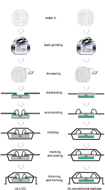
There are two types of IC packaging, namely ceramic and plastic. Most of the commercial IC chips use plastic packaging. For the IC assembly factory mainly producing memory prod-ucts, the conventional packages and thin small outline package, type 2 (TSOP2) package dominant the production lines. Fig. 2 shows the process flows of conventional packages and TSOP2 packages. As we can see in Fig. 2, the process flows of conven-tional packages and TSOP2 packages are the same. Actually, in the floor shop, the machines at each stage can process the op-erations for these two packages, except for at the die bonding stage. For conventional packages, the die bonding process is to position the good dies on the paddle of the leadframe (using epoxy). While, for TSOP2 packages, the die bonding process is lead on chip (LOC), which the device is fixed with an LOC tape underneath the leadframe, and no curing is needed. There-fore, due to the machine difference and cost consideration, the capacity expansion of the die bonder is usually carefully evalu-ated. Though the critical resources in most IC assembly facto-ries are die bonders and wire bonders [4]–[6], for memory prod-ucts, the package lead count of each die is relatively small, and the throughput of the wire bonders is satisfied. Therefore, in the assembly facility mainly producing memory products, the die bonders are treated as the bottleneck.
In contrast to the front-end processes that are highly re-en-trant, the back-end process follows a more linear, assembly-line type of flow [6], [7]. In the ICASP, the bottleneck (the die-bonders) is scheduled to be utilized as efficiently as possible, and this implies the reduction of number of setups is crucial. After completing the scheduling on the bottleneck, the lot re-lease time and the scheduling on all the non-bottlenecks facili-tate the feeding of the bottleneck.
Since the IC assembly scheduling problem involves con-straints on processing priority, job cluster, job-cluster dependent processing time, machine capacity, and sequentially dependent setup times, it is more difficult to solve than the classical par-allel-machine scheduling problem. In this paper, we consider a more general version of ICASP and formulate the ICASP as an integer programing problem. The programing model considers the processing priority constraint, and the processing time and the setup time in the capacity constraints. An efficient heuristic is also proposed to obtain the near-optimal solution for large-scale problems.
Fig. 1. Four stages of the IC manufacturing.
Fig. 2. Process flows of plastic packaging products.
II. LITERATUREREVIEW
The recent increase in device complexity has led to the devel-opment of complex capital-intensive assembly systems. The de-velopments in the area of planning and scheduling IC assembly operations, therefore, have seized more attention from the aca-demic world than before. Liu et al. [4] developed a computer-aided scheduling system. Potoradi et al. [5] developed a simu-lation-based scheduling to maximize demand fulfillment. Liu et al. [8] developed a lot release methodology for minimizing ma-chine conversion. Yin et al. [9] developed a rule-based finite-ca-pacity daily scheduling system. Tovia et al. [6] considered a simple version of the ICASP for the high production volume and
high production mix environment and provided a mathematical model. Tovia et al. [6] also presented a rule-based heuristic ap-proach to solve the problem approximately. Unfortunately, their models do not consider sequence-dependent setup times and job processing priority simultaneously, which may not reflect the real situation accurately.
A number of papers addressed the machine scheduling involving sequence-dependent setup times. Lee and Pinedo [10] considered the identical parallel machine problem with sequence-dependent setup times. Schutten and Leussink [11] presented a branch-and-bound algorithm for solving the iden-tical parallel machine problem with release date, due dates, and family setup times, with the objective of minimizing the max-imum lateness of any job. Webster and Azizoglu [12] presented two dynamic programing algorithms for solving the identical parallel machine problem with family setup times to minimize total weighted flowtime. Dunstall and Wirth [13] proposed a branching scheme to the identical parallel-machine problem with family setups to minimize the weighted sum of comple-tion times. Chern and Liu [14] constructed five family-based scheduling rules, and built a simulation model to examine these five rules. In those research works, the constraint of multiple processing priorities has never been considered; therefore, their models may not be applicable to the ICASP.
The survey papers [15], [16] provide a wide range of par-allel-machine scheduling with precedence constraint. However, the precedence relations studied in these papers can be pre-sented by graphs in tree-types: in-tree type precedence (each job has at most one successor), out-tree type precedence (each job has at most one predecessor), and chain-type precedence (each job has at most one predecessor and at most one successor). In the ICASP, the jobs are completely partitioned and a prece-dence relation defined by the processing priority. Therefore, the algorithms for solving scheduling problems with tree-type precedence constraint may not be applied to the ICASP. Cheng and Diamond [17] considered the parallel machine scheduling problem for minimizing total flowtime, and provided a dynamic programing algorithm. Unfortunately, their model is developed only for two-class priority and does not consider the sequen-tially dependent setup times.
The parallel-machine scheduling problem with precedence constraints and sequence-dependent setup times is a combi-nation of a partitioning (assigning jobs to machines) and a sequencing (sequencing the jobs on each machine) problem. Hurink and Knust [18] considered this parallel machine problem of the objective of minimizing the makespan. Hurink and Knust [18] concluded that no efficient list scheduling algorithm can lead to a dominant set of schedules, and recommended that the solution approach needs to consider partitioning and se-quencing simultaneously.
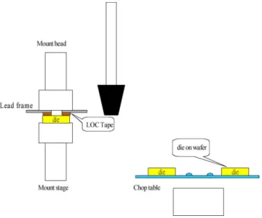
Fig. 3. Die bonding on the LOC die bonder.
III. DESCRIPTION OFICASP
The IC assembly scheduling problem is to seek a schedule for the jobs to be processed in the time horizon, which min-imizes the total die bonder workload, satisfying the job pro-cessing priority without violating the machine capacity con-straint. In ICASP, the jobs are processed on groups of identical die bonders, and the total processing time is constant. Thus, re-ducing the total setup time is essential to the minimization of the total machine workload. Process characteristics modeled in-clude sequence dependent setup times, processing priority con-sideration, and machine capacity constraint.
These integrated circuits, or dies, are formed on wafers that are typically grouped into lot sizes of 25. The size of each lot may vary which depends on the design of dies and die yield. Note that, at the die bonding stage, a lot flowing into the die bonding area is in the form of a complete wafer, and it flows out of this area in the form of a die on leadframe.
A. Sequence-Dependent Setup Times
Since different types of dies must be operated on the LOC die bonder with some specific size of chop table, mount head, and mount stage, and some parameter setting on the machines, some setup operations may be required. Fig. 3 shows the die bonding on the LOC die bonder. The requirement for parameter settings can be regarded as a fixed constant. In the situation, where the current job is formed on 12-in wafers, and the next job is formed on 8-in wafers, and vice versa, the next job would have to put on hold until the chop table is changed. Furthermore, in the situation, where the current job is performed with a small mount head and mount stage and the die size of next job is large, the next job would have to be put on hold until the mount stage and mount head is changed.
Thus, the setup time required for switching one product type to another depends on the size of wafer and die. As the jobs come from several product families with each family including a few product types, switching a job to another among different product types within the same product family only requires the
parameter setting operations on the machine. In other cases, switching a job from one to another among different product types from different product families must consider the total cor-responding setup time occurring due to changing the chop table, changing mount stage and mount head, and the parameter set-ting operations on the machine.
B. Processing Priority Consideration
Due to different product profit rates and the varied impor-tance level of customers, there often exist more than one pri-ority level of orders in most semiconductor companies. Based on the processing priority, for any two jobs scheduled on the same machine, job A with higher processing priority must be completed before job B with lower processing priority can be begun. Throughout this paper, we assume that each lot is as-signed a value of processing priority, which is known at the be-ginning of the planning horizon. The assignment of processing priority method is beyond the scope of this work, and we refer the interested reader to [5] and [8] for approaches to assign pri-ority value.
C. Machine Capacity Constraint
Normally, the lead time for the total assembly portion is 4 to 6 days. By deducting the setup times and processing times on the non-bottleneck machines, the time horizon of the bottleneck is set to 2 days. Due to the variety of lot size and the importance of the process lot in the initial status, a rolling horizon approach is used in the ICASP. In addition, the preventive maintenance (PM) may be frequent and time consuming. When PM of ma-chine is scheduled to perform in the planning horizon, we need to deduct the times from the available machine capacity and update the initial status. In real-life applications, the pacity for each machine can be set based on the available ca-pacity in the time horizon, and the processing time unit can be “minute” or “hour.” Throughout this paper, we have set the “minute” as the unit of the processing time, setup time, machine workload, and machine capacity in our investigation.
Problem Complexity: The ICASP is NP-hard. Even without the multiple processing priority constraint, the ICASP special case which minimizes makespan on a single machine in the presence of sequence-dependent setup times is equivalent to the Traveling Salesman Problem, and it has been shown to be NP-hard [3], [19].
IV. INTEGERPROGRAMMINGFORMULATION
A mathematical programing formulation is a natural way to solve machine scheduling problems [20]. The IP formulations for ICASP have been investigated, but our IP formulation in-cludes both sequentially dependent setup times and processing priority conditions at the same time; therefore, is considerably more complicated than those in [6].
We first define containing
clusters of jobs, each job cluster
containing ( ) jobs to be processed and one pseudojob ( ) which is used as the initial status of a machine. Thus, job cluster contains one pseudojob,
job cluster contains jobs,
and job cluster contains jobs. We also define as the set of pro-cessing priority code containing priority levels. Let ( ) be the processing priority code of job . This code is in the form of a non-negative integer, in such a way, a smaller priority code of job indicates that this job has a higher
pro-cessing priority. Thus, set if job
has a higher processing priority than job .
We also define as the group of
machines containing a set of identical machines. Let be the predetermined machine capacity expressed in terms of processing time unit. Further, let be the lot size of job , and be the unit processing time for each job in cluster ( ) on machine . Therefore, the job processing time for job is . Let be the sequence-dependent setup time between any two consecutive jobs and from different job clusters ( ). Note that the priority codes and lot size for the job should be set to zero so that these pseudojobs should be scheduled as the first jobs on each machine, which indicates the initial status of each ma-chine.
Let be the variable indicating whether the job is scheduled on machine , with if job is sched-uled on machine , and otherwise. Let be the precedence variable defined on two jobs and sched-uled on machine , with if job precede job (not necessarily directly), and otherwise. Let
be the direct-precedence variable defined on two jobs and scheduled on machine , with if job direct precede job , and otherwise.
To find a schedule for the jobs which minimize the total ma-chine workload without violating the mama-chine capacity and pro-cessing priority constraints, we consider the following integer programing model. Although the first summation term (the total processing time) in the objective function of the integer graming model is constant, it is necessary to be used to pro-vide the information of total machine workload in the solutions because managers prefer to know the total machine workload instead of only the total setup time. In addition, with the cessing time included in the objective function, the integer pro-graming model can be used to solve a more general ICASP problem, where the machines are unrelated.
Minimize subject to for all (1) for all (2) for all (3) for all (4) for all (5) for all (6) for all (7) for all (8) for all (9) for all (10) for all (11) for all (12) for all (13) for all (14) for all (15) for all (16) for all (17)
The objective function seeks to minimize the sum of the total processing time and the total setup time over the identical machines. The constraints in (1) assigns the initial status of each machine . For example, in the situation, where the initial status of machine is pseudojob , we will assign and . The constraints in (2) guarantee that only one pseudojob is scheduled on a machine. Constraints in (3) guarantee that job is processed by one machine exactly once. The constraints in (4) state that each machine workload does not exceed the machine capacity.
The constraints in (5) ensure that the precedence variables
and should be set to zero ( )
if any two jobs and are not scheduled on the machine ( ). The number is a constant, which is chosen to be sufficiently large so that the constraints in (5) are satisfied for ( ). The constraints in (6) and (7) ensure that the precedence variables and should be set to zero ( ) if any two jobs
and are not scheduled on the same machine . The constraints in (6) indicates the case that job is scheduled on machine and the job is scheduled on another machine
( ), and the constraints in (7) indicates the case that job is scheduled on machine , and the job is scheduled on another machine ( ). The constraints in (8) and (9) ensure that one job should pre-cede another if two jobs and are scheduled on the same machine ( ). In the situation where these two jobs have the same priority code ( ), the con-straints in (8) and (9) ensure that one job should precede an-other ( ). In the situation where these two jobs have different priority codes ( ), the con-straints in (8) and (9) ensure that job with smaller priority code (higher processing priority) should precede the other job with larger priority code (lower processing priority) (
and if ) or ( and
if ). The constraints in (10) ensure that the job precedes job ( ) when the job precedes
job ( ) and the job precedes job
( ).
The constraints in (11) ensure that job could precede job
directly ( ) only when and job
could not precede job directly ( ) if job is scheduled after ( ). The constraints in (12) state that there should exist direct-precedence variables, which are set to one, on the schedule with jobs. The constraints in (13) guarantee that at most one job could be scheduled after job directly for all the jobs scheduled on the same ma-chine . The constraints in (14) guarantee that at most one job could be scheduled precede job directly for all the jobs scheduled on the same machine .
In the aforementioned integer programing formulation, the total number of variables and equations increase as the number of machines or the number of jobs increase. The computational complexity of the integer programing model is as follows. For a parallel-machine problem with job clusters and machines, containing a total of
jobs, the integer programing model contains variables
of , variables of , and
variables of . Further, the constraint sets in (1), (2), (4), and (12) each contains equations, the constraint set in (3) contains equations, constraint sets in (5)-(9) and (11) each contains equations, the constraint sets in (10) contains equations, and the constraint sets in (13) and (14) contains . Thus, the total number of variables is , and the total number of
equations is .
To accelerate the execution in solving the integer programing problem, we use both a depth-first search strategy by choosing the most recently created node, and a strong branching rule causing variable selection based on partially solving a number of subproblems with tentative branches to find the most promising branch. By using the depth-first search strategy, when the tree size or the number of fully developed branches exceeds limi-tations induced by computation time or memory requirements, the program terminates and returns the best solution achieved. The implementation thus allows us to set various limits on the number of memory nodes so that feasible solutions may be ob-tained efficiently within reasonable amount of computer time. The node limit is set to determine the maximum number of
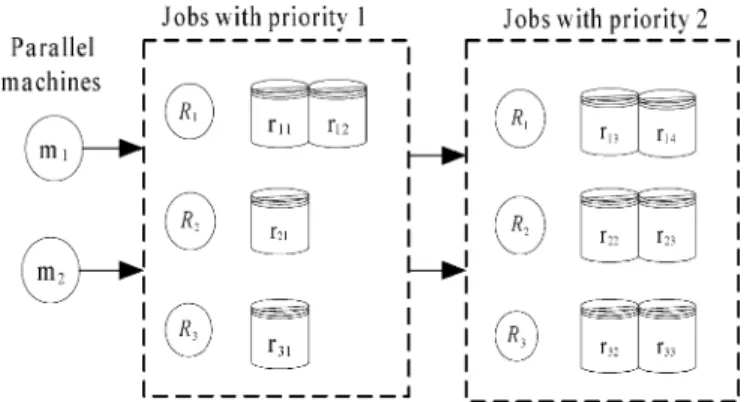
Fig. 4. ICASP example with two parallel machines, two priority levels, and three job clusters.
TABLE I
SETUPTIMESREQUIRED FORSWITCHINGONEPRODUCT
TYPE TOANOTHER FORR , R ,ANDR
TABLE II
JOBPROCESSINGTIMES FORR , R ,ANDR ON THEMACHINESm ANDm
nodes solved before the program terminates, without reaching optimality [21].
V. SOLUTIONS FOR THEICASP
Consider the following ICASP example with two parallel ma-chines ( and ), two processing priority levels (1 and 2, in which a job with priority 1 has a higher processing priority than the jobs with priority 2), and three clusters of jobs ( , , and ) ready for processing initially, as shown in Fig. 4. Job cluster contains four jobs, both and with priority 1 and both and with priority 2. Job cluster contains three jobs, with priority 1 and both and with priority 2. Job cluster contains three jobs, with priority 1 and both and with priority 2. Table I displays the setup times required for switching one product type to another for the three types 1, 2, and 3. In Table I, the label denotes that the machine is in idle status. Table II displays the job processing times for job clusters , , and on the machines and . Note that the setup times and the processing times are associated with the product types, regardless of processing priority levels. The capacity of each machine is set to 140 min in this example. The initial status of machine is , and that of machine is .
To solve the integer programing problem for the ICASP ex-ample, we adopt ILOG OPL [21] to generate the constraints and variables of the model. For the ICASP example with two ma-chines, two processing priority levels, three job clusters, and ten jobs, the model contains 756 variables and 6626 equations. We run the integer programing model using the IP software ILOG
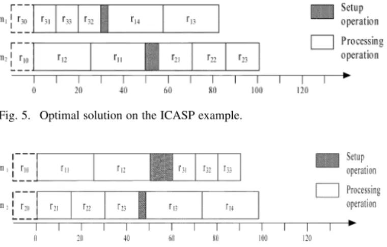
Fig. 5. Optimal solution on the ICASP example.
Fig. 6. Optimal solution on the ICASP example with initial status ofr and r .
CPLEX on a Pentium IV 3.0-GHz PC. The optimal solution for this example is shown in Fig. 5. The total machine workload is 184. For machine , the total machine workload is 83 with setup time 3 and processing time 80. For machine , the total machine workload is 101 with setup time 6 and processing time 95.
Note that the solution will be different when the initial sta-tuses of machines are different. When the initial status of ma-chine is and that of machine is , the optimal solu-tion will become 188, as shown in Fig. 6. For machine , the total machine workload is 90 with setup time 10 and processing time 80. For machine , the total machine workload is 98 with setup time 3 and processing time 95.
As we can see from the solutions of these two examples, in the situation where the initial status of machine is and that of machine is , the first job scheduled on is and the first job scheduled on is . Total machine workload is 184. In the situation where the initial status of machine is and that of machine is , the first job scheduled on machine becomes , and the first job scheduled on becomes . The total machine workload becomes 188.
VI. HEURISTICALGORITHM
For large-scale problems, the depth-first strategy can solve the problem with more computation effort. However, if the com-putational run time is primary concern, the following heuristic algorithm may be considered.
The proposed algorithm essentially consists of two phases. Phase I creates a multiple of machine schedules simulta-neously by finding the feasible job with the smallest setup times to add it to the end of partial schedule PS . Note that a job is feasible and is added to the machine schedule only if the capacity constraint and the processing priority restric-tions are not violated. After Phase I, partial schedules like
PS should be generated,
in which represents the initial status of the machine , represents the job be scheduled at position on machine , and represents the total number of jobs in the schedule PS . For the jobs left unscheduled in Phase I due to the processing priority constraint, in Phase II, we calculate the insertion cost of every unscheduled job at every possible position of each partial
TABLE III DATASET
TABLE IV SUMMARYRESULTS
schedule to insert the job to the lowest insertion cost posi-tion. Note that a job is inserted into the machine schedule only if the capacity constraint and the processing priority restrictions are not violated. Let be the additional setup cost when job is inserted between position and in schedule . Note that the setup time is determined by the product types, and , of job and .
The procedures of the proposed heuristic algorithm are de-scribed as follows.
Phase I- Schedule construction
Step 1) For each machine , let partial schedule
PS initially.
Step 2) Sort the setup times for all pairs of job type and and create a list in ascending order of magnitude. Step 3) Starting from the top of the setup time list, find
the first feasible link in the list, which can be used to extend the end of without violating the machine capacity constraints and the priority restrictions. If there is a tie for the feasible jobs, choose the job with the highest priority.
Step 4) Repeat Step 3 until no feasible job can be added to extend the end of any PS . If there are jobs left unscheduled, proceed to Phase II. Otherwise, stop. Phase II- Job Insertion
Step 1) For each unscheduled job , first compute its best feasible insertion position, by in each machine’s partial schedule
TABLE V
PRODUCTTYPES, PROCESSINGTIME,ANDPROCESSINGPRIORITY IN THEREAL-WORLDEXAMPLE
Step 2) The job is inserted into the lowest insertion cost position of the machine determined by the
lowest insertion cost .
Step 3) Repeat Steps 1 and 2 until all jobs are scheduled. VII. COMPUTATIONALTEST
In this section, two computational tests are presented. The purpose of the first test is to show the results for the problems of small or moderate size. The second test is the scheduling problem based on real-world applications.
A. Computational Test 1
In this test, computational results were presented by a set of randomly generated test problems, with similar characteristics to industrial data. Twelve jobs are to be completed within two days. Thus, the machine capacity is set to 2880 min. Table III shows the data set used to generate the test problems. We con-sider two values of number of job clusters ( ), two sets of level of priority ( ), and three values of number of ma-chines ( ). The unit processing time for the product types are 40, 45, and 50. The lot size of each job was generated using uniform [10, 15] for three machines, uniform [14, 19] for four machines, and uniform [18, 23] for five machines. Thus, we have a total of 12 combinations of problem parameters. For each combination, we generate ten instances, yielding a total of 120 problems.
The IP model was tested using a computer program coded in ILOG OPL language and solved with ILOG CPLEX on a
Pentium IV 3.0-GHz PC. The heuristic algorithm was coded in Compaq Visual Fortran 6.6. For evaluating the solution quality,
percentage error is employed,
where is the average setup time of the heuristic solution, and is the optimal average setup time obtained from the IP model. Table IV lists the results. The proposed heuristic is effective, and each percentage error is less than 3%.
Using the combination of depth-first search strategy and strong branching rule showed to be powerful. For every test problems of three and four machines in the data set, the optimal solution was reached with the 15 000 nodes created (within 5 min of execution time). For every test problem of five ma-chines in the data set, the optimal solution was reached with the 17 000 nodes created (within 10 min of execution time). B. Computational Test 2
In this section, we consider the following example taken from an IC assembly shop-floor in an IC manufacturing factory located in the Science-Based Industrial Park, Tainan, Taiwan, R.O.C. For the case we investigated, there are 20 product types of TSOP2 packaging being processed on 33 parallel LOC die bonders.
This real example contains 105 wafer lots with processing priority, lot size, and unit processing time, which would be die bonding under certain size of chop table, mount stage, and mount head, as shown in Table V. These jobs are to be completed on the 33 parallel die bonders within two days. Therefore, the machine capacity is set to 2880 min.
The setup time required for switching one product type to an-other depends on the chop table changes, mount stage and mount head changes, and parameter settings, as shown in Table VI. The time to change chop table is 240 min, the time to change mount
TABLE VI
SETUPTIMESREQUIRED FORSWITCHINGONEPRODUCTTYPE TOANOTHER IN THEREAL-WORLDEXAMPLE
stage and mount head is 120 min, and parameter settings is 30 min in this case.
Solving the real-world ICASP by our proposed algorithm (the program codes of the algorithm are written in Compaq Visual Fortran 6.6), the sets of machine schedule are generated. The proposed algorithm takes only 0.07 CPU s to obtain the solution with total machine workload 87 602 with setup time 6480 and processing time 81 122 on 33 die bonders.
VIII. CONCLUSION
In this paper, we considered the ICASP, which is a variation of the parallel-machine scheduling problem and is often found in real-world practice. The ICASP is first described in detail to capture the unique structure and characteristics of the IC as-sembly process. We then formulate the ICASP as an integer pro-graming model to minimize the total machine workload. An effi-cient heuristic algorithm is also proposed for solving large-scale problems. From the computational tests, the performances of the proposed model and heuristic algorithm are quite satisfactory. A real-world example taken from an IC assembly shop-floor in an IC manufacturing factory, where 105 jobs to be processed on 33 machines, is solved by the proposed algorithm to obtain the near optimal solution within 0.07 CPU s.
REFERENCES
[1] R. Uzsoy, C. Y. Lee, and L. A. Martin-Vega, “A review of production planning and scheduling models in the semiconductor industry, part I: System characteristics, performance evaluation and production plan-ning,” Trans. Inst. Electron. Eng., vol. 24, no. 4, pp. 47–60, 1992. [2] R. Uzsoy, L. A. Martin-Vege, C. Y. Lee, and P. A. Leonard,
“Pro-duction scheduling algorithms for a semiconductor test facility,” IEEE
Trans. Semicond. Manuf., vol. 4, no. 4, pp. 270–280, Nov. 1991.
[3] T. Freed and R. C. Leachman, “Scheduling semiconductor device test operations on multihead testers,” IEEE Trans. Semicond. Manuf., vol. 12, no. 4, pp. 523–530, Nov. 1999.
[4] T. H. Liu, A. J. C. Trappey, and F. W. Chan, “A scheduling system for IC packaging industry using STEP enabling technology,” IEEE Trans.
Compon., Packag., Manuf. Technol., vol. 20, no. 4, pp. 256–267, Dec.
1997.
[5] J. Potoradi, O. S. Boon, S. J. Mason, J. W. Fowler, and M. E. Prund, E. Yiicesan, C.-H. Chen, J. L. Snowdon, and J. M. Charnes, Eds., “Using simulation-based scheduling to maximize demand fulfillment in a semiconductor assembly facility,” in Proc. 2002 Winter Simulation
Conf., 2002, pp. 1857–1861.
[6] F. Tovia, S. J. Mason, and B. Ramasami, “A scheduling heuristic for maximizing wirebonder throughput,” IEEE Trans. Electron. Packag.
Manuf., vol. 27, no. 2, pp. 145–150, Apr. 2004.
[7] P. Peter and T. Yang, “Integrated facility layout and material handling system design in semiconductor fabrication facilities,” IEEE Trans.
Semicond. Manuf., vol. 15, no. 3, pp. 91–101, Aug. 2002.
[8] W. Liu, T. J. Chua, T. X. Cai, F. Y. Wang, and W. J. Yan, “Practical lot release methodology for semiconductor back-end manufacturing,”
Production Planning Control, vol. 16, no. 3, pp. 297–308, 2005.
[9] X. F. Yin, T. J. Chua, F. Y. Wang, M. W. Liu, T. X. Cai, W. J. Yan, C. S. Chong, J. P. Zhu, and M. Y. Lam, “A rule-based heuristic finite capacity scheduling system for semiconductor backend assembly,” Int.
J. Comput. Integr. Manuf., vol. 17, no. 8, pp. 733–749, 2004.
[10] Y. H. Lee and M. Pinedo, “Scheduling jobs on parallel machines with sequence-dependent setup times,” Eur. J. Oper. Res., vol. 100, pp. 464–474, 1997.
[11] J. M. J. Schutten and R. A. M. Leussink, “Parallel machine sched-uling with release dates, due dates and family setup times,” Int. J. Prod.
Econ., vol. 46–47, pp. 119–125, 1996.
[12] S. Webster and M. Azizoglu, “Dynamic programing algorithms for scheduling parallel machines with family setup times,” Comput. Oper.
Res., vol. 28, pp. 127–137, 2001.
[13] S. Dunstall and A. Wirth, “A comparison of branch-and-bound algorithms for a family scheduling problem with identical parallel machines,” Eur. J. Oper. Res., vol. 167, pp. 283–296, 2005. [14] C. C. Chern and Y. L. Liu, “Family-based scheduling rules of a
se-quence-dependent wafer fabrication system,” IEEE Trans. Semicond.
Manuf., vol. 16, no. 1, pp. 15–25, Feb. 2003.
[15] T. C. E. Cheng and C. C. S. Sin, “A state-of-art review of parallel-machine scheduling research,” Eur. J. Operational Res., vol. 47, pp. 271–292, 1990.
[16] E. Mokotoff, “Parallel machine scheduling problems: A survey,”
Asia–Pacific J. Oper. Res., vol. 18, pp. 193–242, 2001.
[17] T. C. E. Cheng and J. E. Diamond, “Scheduling two job classes on parallel machines,” Trans. Inst. Electron. Eng., vol. 27, pp. 689–693, 1995.
[18] J. Hurink and S. Knust, “List scheduling in a parallel machine environ-ment with precedence constraints and setup times,” Oper. Res. Lett., vol. 29, pp. 231–239, 2001.
[19] C. Y. Liu and S. C. Chang, “Scheduling flexible flow shops with se-quence-dependent setup effects,” IEEE Trans. Robot. Autom., vol. 16, no. 4, pp. 408–419, Aug. 2000.
[20] A. H. G. R. Kan, Machine Scheduling Problems: Classification,
Com-plexity and Computations. The Hague, The Netherlands: Martinus Nijhoff, 1976.
[21] ILOG OPL Studio 3.6 User’s Manual. Gentilly Cedex, France: ILOG SA, 2002.
W. L. Pearn received the Ph.D. degree in operations research from the University of Maryland, College Park.
He is a Professor of Operations Research and Quality Assurance at National Chiao-Tung Uni-versity (NCTU), Hsinchu, Taiwan, R.O.C. He was with AT&T Bell Laboratories as a member of quality research staff before joining NCTU. His research interests include process capability, network optimization, and production management. His publications have appeared in the Journal of the
Royal Statistical Society, Series C, Journal of Quality Technology, Journal of Applied Statistics, Statistics and Probability Letters, Quality and Quantity, Metrika, Statistics, Journal of the Operational Research Society, Operations Research Letters, Omega, Networks, International Journal of Productions Research, and others.
S. H. Chung received the Ph.D. degree in industrial engineering from Texas A&M University, College Station.
She is a Professor of the Department of Industrial Engineering and Management, National Chiao-Tung University, Hsinchu, Taiwan, R.O.C. Her research interests include production planning, scheduling, cycle time estimation, and performance evaluation. She has published and presented research papers in the areas of production planning and scheduling for IC manufacturing.
C. M. Lai received the Ph.D. degree in indus-trial engineering and management from National Chiao-Tung University, Hsinchu, Taiwan, R.O.C, in 2007.
Her research interests include production plan-ning, scheduling, and cycle time estimation.