異質變異之穩健模型估計

行政院國家科學委員會專題研究計畫 成果報告

異質變異之穩健模型估計

研究成果報告(精簡版)

中 華 民 國 96 年 09 月 17 日

行政院國家科學委員會補助專題研究計畫

■ 成 果 報 告

□期中進度報告

（計畫名稱）

異質變異之穩健模型估計

計畫類別：■ 個別型計畫 □ 整合型計畫

計畫編號：NSC

95

－

2118

－

M

－

004

－0

05

－

執行期間： 2006 年 8 月 1 日至 2007 年 8 月 31 日

計畫主持人： 鄭宗記

共同主持人：

計畫參與人員：

成果報告類型(依經費核定清單規定繳交)：■精簡報告 □完整報告

本成果報告包括以下應繳交之附件：

□赴國外出差或研習心得報告一份

□赴大陸地區出差或研習心得報告一份

■出席國際學術會議心得報告及發表之論文各一份

□國際合作研究計畫國外研究報告書一份

處理方式：除產學合作研究計畫、提升產業技術及人才培育研究計畫、

列管計畫及下列情形者外，得立即公開查詢

□涉及專利或其他智慧財產權，□一年□二年後可公開查詢

執行單位：

國立政治大學 統計學系

Robust Diagnostics for the Heteroscedastic Regression

Model

Tsung-Chi Cheng

September 17, 2007

Abstract

The assumption of equal variance in the normal regression model is not always ap-propriate. Cook and Weisberg (1983) provide a score test to detect heteroscedastic-ity, while Patterson and Thompson (1971) propose the residual maximum likelihood (REML) estimation to estimate variance components in the context of an unbalanced incomplete-block design. REML is often preferred to the maximum likelihood esti-mation as a method of estimating covariance parameters in a linear model. However, outliers may have some effect on the estimate of the variance function. This paper in-corporates the maximum trimming likelihood estimation of Hadi and Luce˜no (1997) in REML to obtain a robust estimation of modelling variance heterogeneity. The forward search algorithm of Atkinson (1994) is employed to find the resulting estimator. Sim-ulation and real data examples are used to illustrate the performance of the proposed approach.

Keywords: Forward search algorithm; heteroscedasticity; maximum trimmed likelihood

estimator; residual maximum likelihood estimator; outlier; robust diagnostics.

1

Introduction

The assumption of equal variance in the normal regression model is not always appropriate. Cook and Weisberg (1983) provide a score test to detect heteroscedasticity. In an attempt to eliminate variance heterogeneity, a transformation is often used, but the evidence for transformations may sometimes depend crucially on one or a few observations. Several authors point out that data transformations can be very sensitive to outliers (eg. Tsai and Wu, 1990). Furthermore, it may be the case that modelling the variance itself is of great interest or a simple transformation is inadequate to correct for the unequal variance.

∗_{Department of Statistics, National Chengchi University, 64 ZhihNan Road, Section 2, Taipei 11605,}

Apart from the maximum likelihood estimation (MLE) for the linear regression model with heteroscedastic error (see Harvey, 1976; Aitkin, 1987), Patterson and Thompson (1971) propose the residual maximum likelihood (REML) estimation to estimate variance compo-nents in the context of an unbalanced incomplete-block design. REML is often preferred to MLE as a method for estimating covariance parameters in a linear model. Alternative and more general derivations of REML are given by Harville (1974), Cooper and Thompson (1977) and Verbyla (1990). Applying the conditional likelihood representation, Smyth and Verbyla (1996) extend the concept of REML to the generalized linear models with varying dispersion and a canonical link. One of the advantages about REML is it provides a tool to estimate the varying variance function during the iterative procedure.

Carroll and Ruppert (1988, chapter 5) discuss issues about regression transformation and weighting in an effort to robustify the analysis. More general discussions on estimating the heteroscedastic regression models are given by Welsh, Carroll and Ruppert (1994). One of the shortcomings in their approaches is that they can have a low breakdown point. Verbyla (1993) extends the deletion diagnostic approach to detect the dependence, estimation, and tests of homogeneity based on full and residual maximum likelihoods. However, it is known that case deletion diagnostics has its limitation in terms of masking and swamping effects when multiple outliers exist in the data. This essentially requires a robust estimator. One of the desirable properties for a robust estimator is one with a high breakdown point that is capable of handling multiple outliers. Several approaches have been proposed for the purposes of the identification of outliers and robust estimation in the last two decades. Among these methods, Hadi and Luce˜no (1997) propose the trimmed likelihood estimator, which is based on trimming the likelihood function rather than directly trimming the data. They refer to this method as the maximum trimmed likelihood (MTL) method and the corresponding estimator as the maximum trimmed likelihood estimator (MTLE).

M¨uller and Neykov (2003) discuss the relationships of the least trimmed squares (LTS) estimator and MTLE for a generalized linear model. Employing the concepts of the least trimmed squares (LTS) estimator and the maximum trimmed likelihood estimator (MTLE), Cheng (2005) unifies robust statistics and a diagnostic approach to deal with the outlier problem in the regression transformation. Cheng and Biswas (2007) apply the MTL approach to obtain the robust estimators of the multivariate location and shape, especially for data mixed with continuous and categorical variables. The purpose of this article is to develop a robust method of modelling variance heterogeneity that will not be influenced by potential outliers.

estimation for the problem of variance heterogeneity when outliers are present in the data. This paper is outlined as follows. Section 2 briefly reviews the literature about modelling heteroscedasticity for the linear regression model. Section 3 discusses the idea of the trimmed likelihood approach. A new estimation procedure is then proposed in combination with both REML and MTL approaches, which is named as the residual trimmed maximum likelihood (RTML) estimator. It is given in oreder to deal with estimating the heteroscedastic regres-sion model in the presence of outliers. The forward search algorithm of Atkinson (1994) is adapted for the resulting RTML estimator. Section 4 conducts a simulation study to com-pare the performance of the REML and RTML estimators. Section 5 illustrates the proposed procedure using three real data examples. New findings are discovered by the RTML results. Section 6 concludes.

2

Model of heteroscedasticity

Consider the linear model

yi = xTi β + ²i, i = 1, 2, · · · , n, (1)

where yi is the response variable, xi is a p × 1 vector of explanatory variables, β is a vector

of unknown parameters, and ²i is the random error that is assumed to be independent and

follows N(0, σ2

i(γ)). The variance model is the log-linear form

log σ2

i = zTi γ, (2)

where zi is a k × 1 vector of explanatory variables and γ is a vector of unknown parameters.

It is noted that zi may and often does have common components as xi. The first component

of each zi is 1, so that if γ2 = · · · = γk = 0, then this leads to a constant variance σ2 = exp γ1.

2.1

Maximum likelihood estimation

The maximum likelihood estimation for the heteroscedastic regression model has been dis-cussed by Harvey (1976) and Aitkin (1987), which is briefly described as follows. The log-likelihood under models (1) and (2) is

log L(β, γ; y) = −1 2 ( _n X i=1 log σ_i2+ n X i=1 (yi− xTi β)2 σ2 i ) , (3)

where y be a n × 1 vector of the response variable. Let d be the vector with ith element

respectively, and Σ is the diagonal variance matrix with ith element σ2

i. If 1n denotes the

n × 1 vector of unit elements, then the score vector and the Fisher expected information of (3) are u(β, γ; y) = Ã XTΣ−1(y − Xβ) 1 2Z T_(Σ−1_{d − 1} n) ! and I(β, γ) = Ã XTΣ−1X 0 0 1 2Z T_Z ! . (4)

This yields an iterative procedure for the estimates as ˆ

β_(t+1) = (XTΣ−1_(t)X)−1XTΣ−1_(t)y, ˆ

γ_(t+1) = ˆγ_(t)+ (ZT_Z)−1_ZT_(Σ−1

(t)d − 1n),

where t indicates the tth iterate. Cook and Weisberg (1983) provide a diagnostic test based on results (4) for a non-constant variance of models (1) and (2).

2.2

Residual maximum likelihood estimation

With a variance model, REML takes into account the loss of degrees of freedom in estimating the mean. The REML estimate of γ is founded by using the marginal likelihood (Patterson and Thompson, 1971; Harville, 1974; Cooper and Thompson, 1977; Verbyla, 1990 and 1993)

log LR(γ; y) = −1 2 n log |Σ| + log |XTΣ−1X| + yTP yo = −1 2 ( _n X i=1 zT_i γ + log |XTΣ−1X| + yTP y ) , (5)

where P = Σ−1_{− Σ}−1_X(XT_Σ−1_X)XT_Σ−1_{. The score vector for γ is given by}

uR(γ) =

1

2Z

T_(Σ−1_{d − 1}

n+ h),

where h is the vector of the diagonal elements of

H = Σ−1/2X(XTΣ−1X)−1XTΣ−1/2.

This is the hat matrix in a weighted regression. The expected information matrix is

IR(γ) =

1

2Z

T_{V Z,}

where V = V ar(Σ−1_{d)/2. V is an n × n matrix with diagonal elements (1 − h}

ii)2 and

off-diagonal elements h2

ij, where hij denotes the (i, j) entry of H.

The method of scoring leads to the estimate when evaluated at iterate t as being ¯

γ_(t+1) = ¯γ_(t)+ (ZTV Z)−1ZT(Σ−1_(t)d − 1n+ h).

REML is often preferred to MLE as a method of estimating covariance parameters in the linear model. An R package, statmod, is provided by Smyth (2002) to fit heteroscedastic and varying dispersion models by REML.

3

Robust heteroscedastic regression model

It is known that outliers can have effects on REML (eg. Verbyla, 1993). Therefore this section considers a robust estimation for the heteroscedastic regression model. The method extends the maximum trimmed likelihood approach to REML.

3.1

The maximum trimmed likelihood estimator

Hadi and Luce˜no (1997) propose a trimmed likelihood principle based on trimming the likelihood function rather than directly trimming the data. It is always possible to order and trim observations according to their contributions to the likelihood function, because the likelihood is scalar-valued. For any given value of θ,

l(θ; x1) ≥ l(θ; x2) ≥ · · · ≥ l(θ; xn), (6)

where l(θ; xi) = ln f (xi; θ) is the contribution of the ith observation to the log likelihood

function. Therefore, the ML estimator maximizes the log likelihood function as

n

X

i=1

l(θ; xi).

The method proposed by Hadi and Luce˜no (1997) replaces the log likelihood function by the trimmed log likelihood function:

b

X

i=a

wil(θ; xi), (7)

where a ≤ b, (a, b) ∈ {1, 2, · · · , n}, and wi ≥ 0 are weights. The estimator θ(a, b, w) is

obtained by maximizing (7). They call this method as the maximum trimmed likelihood

(MTL) method and ˆθ(a, b, w) is the maximum trimmed likelihood estimator (MTLE).

Hadi and Luce˜no (1997) show that this trimming likelihood principle produces many ex-isting estimators, such as MLE, least median squares (LMS), least trimmed squares (LTS), and minimum volume ellipsoid (MVE) estimators. Cheng and Biswas (2007) present the re-lation of MTLE with the minimum covariance determinant (MCD) estimator for multivariate data.

3.2

Residual trimmed maximum likelihood estimation

In combination with both MTL and REML approaches, we propose a residual trimmed

the parameters for a specific value of q. If Q denotes the subset with q cases and the

corresponding data are denoted by y_qand Xq, then the trimmed log-likelihood under models

(1) and (2) is log Lq(βq, γq; yq) = − 1 2    X i∈Q log σ2 qi + X i∈Q (yi− xTi βq)2 σ2 qi   . (8)

The corresponding RTML estimator is analogous to (5), which is to maximize log LRq(γq; yq) = − 1 2 n log |Σq| + log |XTqΣ−1q Xq| + yTqPqyq o = −1 2    X i∈Q zT i γq+ log |XTqΣ−1q Xq| + yTqPqyq   , (9)

where Pq = Σ−1q − Σ−1q Xq(XTqΣ−1q Xq)XTqΣ−1q and Σq is the diagonal variance matrix with

ith element σ2

qi. The resulting RTML estimator evaluated at q is denoted by ˆθq = (ˆβq, ˆγq).

This corresponds to the REML estimator based on the subset Q. Therefore, the analogous expression of the score vector and expected information matrix for γ remain the same in subsection 2.2. The details are expressed in the subsequent subsection. The difficulty here is to find the subset Q.

3.3

Computing algorithm

To obtain the RTML estimate of θq, this subsection employs the forward search algorithm

of Atkinson (1994). The forward search algorithm starts with a randomly selected subset of observations. The observations of the subset are incremented in such a way that outliers are unlikely to be included.

For a specific value of q, we now give the details about using the forward search algorithm to an approximate solution of ˆθq.

• Step 0. Choose the initial subset:

The forward search algorithm starts with the selection of a subset of m = m0 units,

where m0 must be large enough to estimate the unknown parameters θ. Here, we

suggest using m0 = p + k. The subset is denoted by M.

• Step 1. Obtain the ordered log-likelihood:

We first compute the REML estimate of θ based on the subset M, which is to maximize log LRm(γm; ym) = − 1 2 n log |Σm| + log |XTmΣ−1m Xm| + yTmPmym o , (10)

where Pm = Σ−1m − Σ−1m Xm(XmTΣ−1m Xm)XTmΣ−1m . The method of scoring leads to the

estimate when evaluated at iterate t as ˆ β_m,(t+1) = (XT_mΣˆ−1_m,(t)Xm)−1XTmΣˆ −1 m,(t)ym, ¯ γ_m,(t+1) = ¯γ_m,(t)+ (ZT mVmZm)−1ZTm( ˆΣ −1 m,(t)dm− 1m+ hm).

Here, hm is the vector of the diagonal elements of the corresponding hat matrix

Hm = ˆΣ −1/2 m,(t)Xm(XTmΣˆ −1 m,(t)Xm)−1XTmΣˆ −1/2 m,(t),

where ˆΣm,(t) denotes an m × m matrix with the ith diagonal element ˆσmi2 . Moreover,

Vm is an m × m matrix with diagonal elements (1 − hii)2 and off-diagonal elements

h2

ij, where hij denotes the (i, j) entry of Hm, and dm is the vector with ith element

di = (yi− xTi βˆm,(t))2, i ∈ M.

The resulting estimate is denoted by ˆθm = (ˆβm, ¯γm). Here, ˆθmcan be directly obtained

by using Smyth’s (2002) approach based on the chosen m observations. We then calculate the value of the log-likelihood for each case as:

lim(ˆβm, ¯γm) ∝ − 1 2 ( zT i γ¯m+ (yi− xTi βˆm)2 ˆ σ2 mi ) , i = 1, · · · , n, (11) where ˆσ2 mi= zTi γ¯m.

• Step 2. Calculate the value of the objective criterion:

The objective function of the RTML estimation evaluated at q is `qm =

q

X

i=1

l(i)m, (12)

where l(i)m is the ordering of the log likelihood lim as

l(1)m ≥ l(2)m ≥ · · · ≥ l(n)m. (13)

• Step 3. Add observations during the forward search:

Let m = m0+ s (usually s = 1). We then choose those cases with the largest m values

of the ordered log-likelihood (13). These new m cases form a new subset, also denoted by M.

• Step 4. Iterate Step 1 to Step 3 until the size of the subset equals n:

At each forward iteration, a new REML estimate ˆθm is obtained from the new subset,

and hence so is the value of the log-likelihood (11), lim, for i = 1, 2 · · · , n and ordering

l(i)m. As a sequence, this leads a series of `qm, m = m0+ s, m0+ 2s, · · ·. The maximum

Steps 0 to 4 form a forward search. One hundred forward searches are suggested by

Atkinson (1994), which yield a series of `q’s. The maximum value of these `q’s provides the

approximate solution of the RTML estimate of θ, which is also indicated by ˆθq for simplicity.

It is noted that the resulting RTML estimate can be viewed as the REML one based on those q observations.

Once ˆθq is obtained, the so-called weighted residual

si = ei ˆ σqi = yi− x T iβˆq ˆ σqi , i = 1, 2 · · · , n, (14)

can be used to flag the outlying cases. Here, ˆσ2

qi = zTi γ¯q, i = 1, 2 · · · , n. The corresponding

hat matrix is then

Hq = ˆΣ −1/2 q(n)X(XTqΣˆ −1 q Xq)−1XTΣˆ −1/2 q(n) ,

where ˆΣq(n) denotes an n × n matrix with the ith diagonal element, ˆσqi2, and ˆΣq denotes an

q × q matrix corresponding to those q cases in the chosen subset. Let hqi denote the ith

diagonal element of Hq. It can be used to identify the leverage point.

4

Simulation study

In this section we conduct a simulation study to show the performance of the proposed approach.

4.1

Data generating process

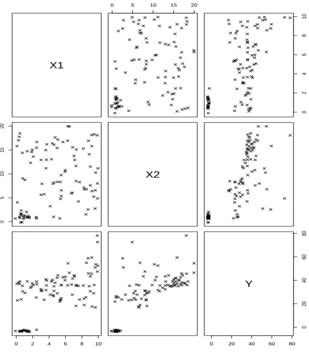
To generate data for the heteroscedastic regression model with high leverage points, we adapt the process of Rousseeuw (1984), in which a well-known simulated data example for the linear regression model with high contamination is present. To illustrate the proposed

approach, p = 2 is used. For “good” data, x1 is generated from the uniform distribution

U(0, 10) and x2 follows U(0, 20), and the response variable is as follows

yi = 20 + x1i+ x2i+ ²i,

where ²i ∼ N(0, σi2) and

log σ_i2 = 0.001 + 0.6x1i.

The “bad” data points are generated from a multivariate normal distribution    x1 x2 y   ∼ MN       1 1 ym− 20   ,    0.252 _{0 0} 0.252 ₀ 0 0.252      ,

where ym denotes the smallest values of those good yi’s.

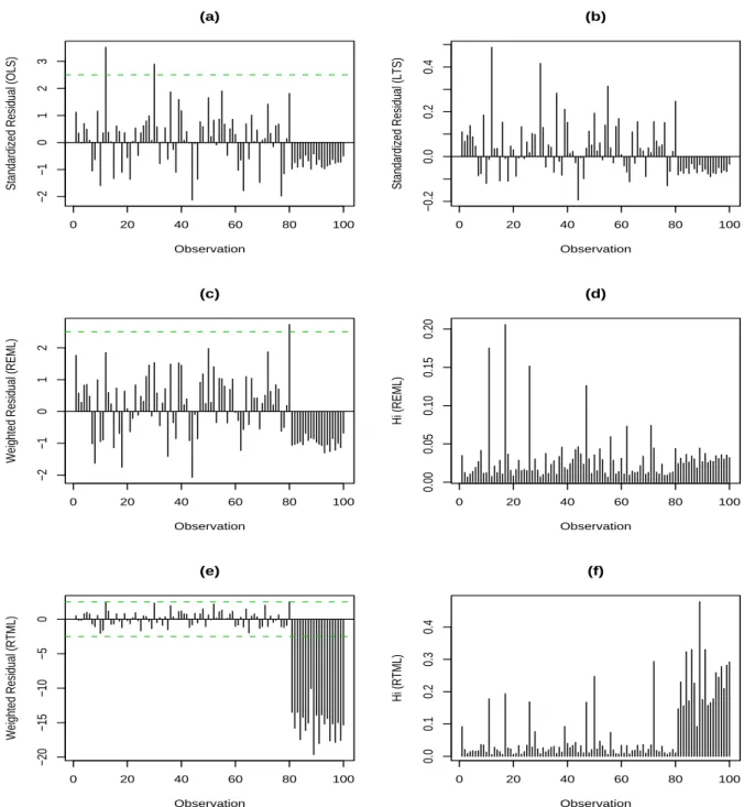
Figure 1 presents the scatter matrix of the simulated data with sample size 100, in which the last 20 observations are assigned to be outlying. Parts (a) and (b) of Figure 2 are the standardized residuals computed by OLS and LTS (75% of data used for the fitting), respectively. There is no outlier revealed by LTS, whereas OLS identifies a couple of points as outliers. Parts (c) and (e) of Figure 2 are the weighted residuals computed by the REML and RTML approaches, respectively. Only one case revealed as an outlier based on REML,

while those 20 outlying cases are successfully identified by RTML. The values of hi obtained

by REML and RTML are shown in parts (d) and (f) of Figure 2, respectively. They result in quite different patterns by these two approaches.

===Figure 1 is here=== ===Figure 2 is here===

4.2

Simulation result

To see the capability of the proposed procedure, we conduct a simulation for models (1) and (2). The data are generated in a similar manner as the previous subsection. The good

data are generated by model (1) setting parameter β0 = 20 and all other β’s being 1. The

values of x1 are generated from a uniform distribution with values between 0 and 10, while

other x variables have values between 0 and 20. In order to simplify the study, p = 5 is used

and only one explanatory variable, x1, is related to the error function. The heteroscedastic

errors follow (2) using the parameter values as γ0 = 0.001, and γ1 = 0.3, 0.6, or 0.9 (for the

different values of γ1, denoted by data types I, II and III, respectively). All other γ’s are then

zero. The values of γ1 are assigned to produce a relatively moderate to a very severe degree

of heteroscedasticity, while the “bad” data are generated from a multivariate distribution with the following form

à xT i yi ! ∼ MN Ãà 1T ym− 20 ! , diag(0.252_{, · · · , 0.25}2₎ ! ,

where ym denotes the smallest values of those good yi’s. This will allow more distinct

distances between bad and good data for more heteroscedastic data. It is noted that the simulated data belong to data type II. The range of data type III is larger than the other two types, so that those outlying points will be farther away from the good data at the same values of x1.

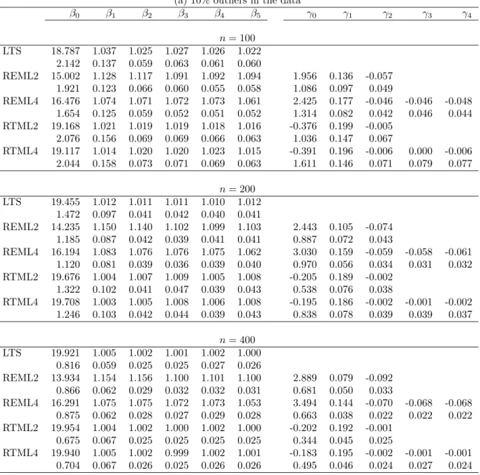
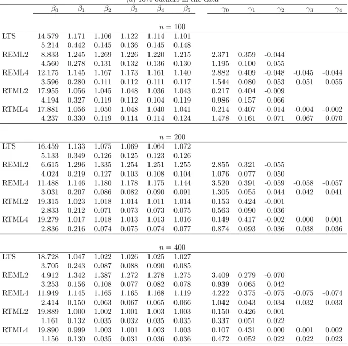
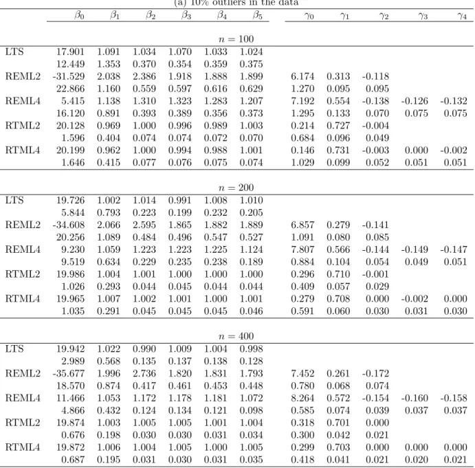
The comparison between REML and RTML is the main concern herein. Tables 1, 2, and 3 present the simulation results of data types I, II, and III, respectively. For each data type,

sample sizes 100, 200, and 400 are considered. Each data set contains 10% or 20% outliers, and 300 replicates are carried out to compare the average estimates of β and γ, which are shown on the first line in the tables. The values on the second line for every β and γ are the sample standard deviation of the 300 estimates. To examine the effects of variance functions,

two kinds of error functions are considered in the model fitting. One includes regressors X1

and X2, and the other considers the extra effect of X3 and X4. REML2 and RTML2 denote

the former, while REML4 and RTML4 indicate the latter. ===Table 1 is here=== ===Table 2 is here=== ===Table 3 is here===

It is clear to see that RTML outperforms REML, especially when heteroscedasticity becomes more severe. For every data type, both RTML2 and RTML4 provide quite close results in estimating the mean functions, whereas the difference between RTML2 and RTML4 becomes larger when the degree of heteroscedasticity is more severe. This may due to the

choice of the error function model. The estimate of γ2 for RTML2 and that of (γ2, γ3, γ4)

for RTML4 are close to zero. This concludes that the different choices of the error functions do not lead to different results by RTML, but do have an effect on estimating variance parameters by REML.

The higher the sample size is, the better the performance of RTML is in terms of both the smaller bias and smaller sample standard deviation. However, the behavior of REML does not depend on the sample size when outliers exist.

It is noted that the LTS (under the assumption of constant errors) provides quite reason-able results when the sample size is large, but the sample standard deviations are relatively large. This is due to a neglect of the heteroscedastic errors. This becomes serious when the degree of heteroscedasticity is severe (data type III). All results of LTS fit based on 75% of the data.

The results for data type III also seem to be better than the other two data types. This is due to the outliers for type III being more distant than the other two.

Other effects on the performance of the proposed approach are the value of q for the RMTL and the value of s for the forward searches. For the simulation results above, the values of q are set to be [0.75n] for both RTML and LTS, and s is 2, 3, and 6 for sample size 100, 200, and 400, respectively. Atkinson and Cheng (1999) conclude that the higher the value of q is, the higher the efficiency of LTS will be, and the more stable the identification of outliers is, provided that the value of q is not large enough to include the existing outliers. A similar result can be expected for the RTML estimates. On the other hand, the smaller

values of s will consume more computation time. We do not explore both issues further here, but the different values of q will be examined for real data examples in the next section.

5

Examples

In this section three real data examples are used to illustrate the RTML approach.

5.1

Mussels data

Mussels data have been used to illustrate transformations of response and explanatory vari-ables for the regression analysis by Cook and Weisberg (1994). The data were collected as part of a larger ecological study of mussels. There are 82 mussels in this data set. The mass (M) of the mussel’s muscle is measured as the response variable. There are four explanatory variables related to the physical measurements of each mussel’s shell, including the length (L), width (W ), height (H), and mass (S). Apart from the following linear regression model

M = β0+ βLL + βWW + βHH + βSS + ², (15)

Cook and Weisberg (1997) employ the marginal model plot which reveals the nonconstant variance for this model. Therefore, they consider a dispersion model to improve the above mean model as follows

V ar(²|L, W, H, S) = exp(γ0+ γLL + γWW + γHH + γSS). (16)

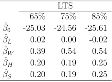
Firstly, two available approaches are suggested to inspect heteroscedasticity. The first one applies LTS regression approach using several different proportions of data to fit the model under the assumption of constant errors. Atkinson and Cheng (1999) present this to evaluate the stability of the estimates and the identification of outliers. Table 4 shows the estimation results by LTS based on 65%, 75%, and 85% of data fitting for model (15). The

estimate of βL varies from the positive sign to a negative sign when the proportion of data

increases in the fitting. The estimate of βW based on 65% of data is different from those

based on 75% and 85% of data. While the estimates of βH and βS remain the same for

65% and 75% of data, different values are obtained when 85% of data are fitted in LTS. The instable estimation may be due to outliers and/or heteroscedastic errors.

===Table 4 is here===

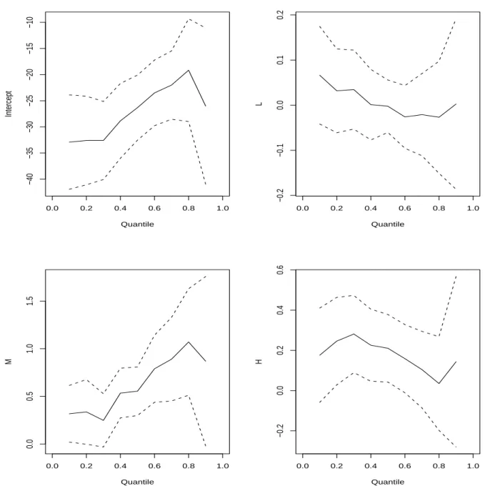
The second approach to reveal heteroscedasticity is to apply the quantile regression anal-ysis of Koenker and Bassett (1978). The test for heteroscedasticity by means of regression

quantiles have been discussed by Koenker and Bassett (1982) and Welsh, Carroll and Rup-pert (1994). Similar to the previous one for LTS, here we also use quantile regression as an exploratory tool rather than confirmatory analysis for revealing heteroscedasticity. Figure 3 presents the estimates evaluated at quantiles 0.1 to 0.9 for model (15) without S. The solid line denotes the point estimate and the dashed lines indicate the bound of the 95% confidence interval for the estimates. These results are obtained through the approach of Kocherginsky, He and Mu (2005). It is clear to see that the values of the estimated coefficient for variable L declines from the lower quantile to the higher one, whereas those for variable M increase from the lower quantile to the higher one. It also features that the confidence intervals of the estimates are wider for higher quantiles. This may imply that heteroscedastic errors exist in the data.

===Figure 3 is here===

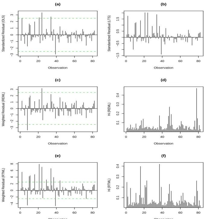
We then apply REML and RTML to these data by fitting models (15) and (16). Parts (a) and (b) of Figure 4 are the plots of the standardized OLS and LTS residuals, respectively, which are based on model (15) under constant errors. Part (c) is the plot of the weighted residuals based on the REML approach. In general, these three residual plots present quite a similar pattern although different outlying cases are identified, while part (e) is the plot of the weighted residuals by RTML. It shows a similar pattern as the previous three plots, but larger values of residuals are given for several observations. Cases 2, 8, 10, 11, 16, 21, 24, 29, 34, 37, 39, and 44 are revealed as outlying by RTML, whereas only cases 8 and 24 are

outliers by REML. Parts (d) and (f) depict the values of hi obtained by REML and RTML,

respectively. However, they appear to be quite different patterns by these two approaches. Apart from model (16), another two variance functions are also examined. Similar results for the identification of outliers are obtained based on the other two models. We omit this part, because there are similar plots as in Figure 4 for these two models. Table 5 presents the estimation results, in which all these three models yield quite similar estimates for the mean function based on each approach, REML and RTML. Nevertheless, the estimates under the same models are quite different between these two approaches.

To verify the difference, a case-deletion based on REML is used. REMLS _{denotes the}

result applying the REML approach based on subset S being excluded from the data. Here,

S1 denotes those 12 outlying observations revealed by RTML, whereas S2 includes 2 outlying

cases by REML. It is clear to see that the results of RTML and REMLS1 are similar, and

there is a slight difference between REML and REMLS1, and REMLS1 and REMLS2 are

quite different from each other. Furthermore, if we look at the values of deviance and the score statistic of Cook and Weisberg (1983), the difference is distinct when fitting the model

without those cases in S1. This also confirms that the score test is clearly influenced by

outliers.

A comparison among these tree models is not significantly different in terms of deviance

for REMLS1 and the objective value for RTML. The latter one is denoted by MTL

q in Table

5, which shows the maximum values of `q’s. It is noted that q = [0.85n] is used for RTML

and LTS for the presentation. Other values of q, such as [0.65n], [0.75n] and [0.9n], have been examined as well, but similar results are obtained.

===Figure 4 is here=== ===Table 5 is here===

5.2

Cherry trees data

The cherry tree data set is used by several authors to illustrate the problems of a regression transformation and a transform-both-sides model. This is a set of measurements on the volume (Y ), diameter (D), and height (H) of 31 black cherry trees. Atkinson (1985, pp. 124-129) compares some candidate models to provide a means of predicting the volume of timber in unfelled trees. If the first-order regression model is considered, which includes the response variable, volume, and two explanatory variables, girth and height, then the score statistic suggests strong evidence of a transformation on the response variable and the

estimated transformation parameter ˆλ = 0.3066. Tsai and Wu (1990) conclude that the cube

root transformation (the quick estimate of Cook and Wang (1983) for λ is 0.2931) to the dependent variable with the weighted regression model provides a reasonable explanation of the data. Cheng (2005) obtains the different estimated values of λ (between 0.21 and 0.36) when different proportions of data are used for LTS, which may be due to the heteroscedastic error structure in the data (Tsai and Wu, 1990). Cook and Weisberg (1983) use the score test to examine several heteroscedastic error functions for these data. Verbyla (1993) also uses these data, but different error functions are inspected. We then explore this data set further here.

According to the previous studies mentioned above, the following model is reasonable for these data

Y1/3 = β0+ βHH + βDD + ².

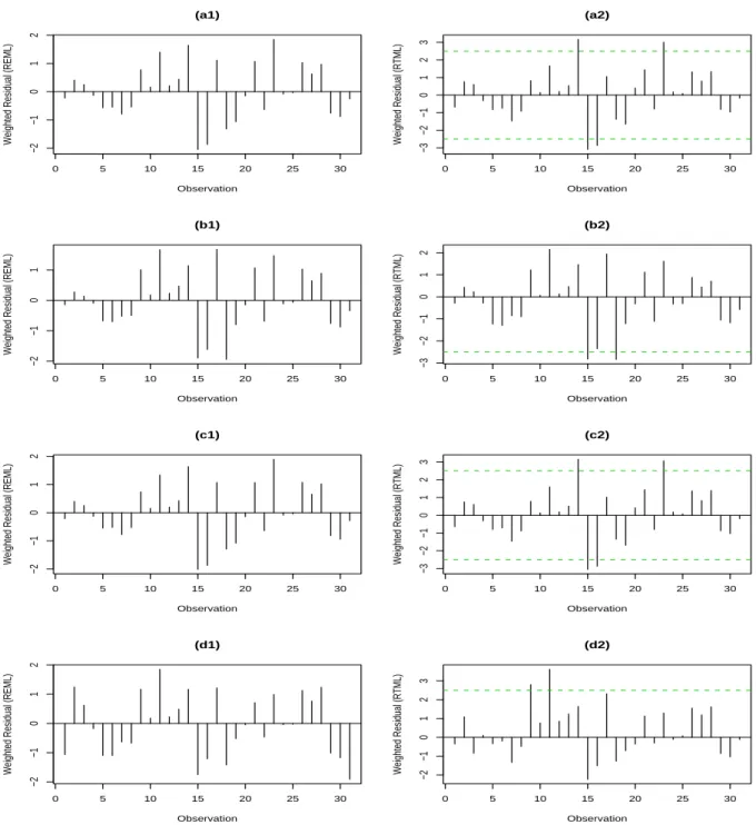
Four kinds of variance functions for the above model are considered as shown in Table 6. Here, models A, B, and C were examined by Cook and Weisberg (1983), while model D was discussed by Verbyla (1993). Figure 5 compares the weighted residuals between REML and RTML for these four models. No matter which model is used, there is no other outlier

revealed by REML as shown in parts (a1), (b1), (c1), and (d1) of Figure 5. However, RTML detects different outliers under different models. For models A and C, cases 14, 15, 16, and 23 are outliers as shown in parts (a2) and (c2) of Figure 5, while part (b2) of Figure 5 flags out cases 15 and 18 as outliers for model B, and cases 9 and 11 for model D in part (d2). The different outliers are identified based on different variance functions. This coincides with the findings of Cheng (2005). He shows that different subsets of deleted cases are obtained when estimating the robust transformation parameter as different proportions of data are used for LTS. The results confirm that this is due to the different heteroscedastic errors.

The case-deletion approach is used again to verify the different results obtained by REML and RTML. Table 6 presents the estimation results. Firstly, no matter what heteroscedastic error structures are considered, the estimates of the mean function for these four models are quite similar based on each approach, REML and RTML. However, the estimates of the coefficients vary for different variance functions. The values of deviance and the score statistic of Cook and Weisberg (1983) are also distinct when those outliers are excluded or included in the analysis.

It is noted that the RTML results based on q = [0.9n] are reported here, and other values of q yield similar results.

===Figure 5 is here=== ===Table 6 is here===

5.3

Gas vapours data

This is a set of experimental data relating the quantity of hydrocarbons recovered (Y ) to

four explanatory variables, including initial tank temperature (X1), temperature of gasoline

(X2), initial vapour pressure (X3), and vapour pressure of dispensed gasoline (X4). It is a

series of 32 fillings of a tank with gasoline for the purpose of studying a device for capturing emitted hydrocarbons. A linear regression model is considered by Cook and Weisberg (1983) as

Y = β0+ β1X1+ β2X2+ β3X3+ β4X4+ ²,

and the assumption of homoscedasticity is examined.

Cook and Weisberg (1982) conclude that there is no other influence case in the data. We reach a similar conclusion when applying the REML approach to these data under four kinds of heteroscedastic errors as shown in parts (a1), (a2), (a3), and (a4) of Figure 4, in which there appear only one or two outlying cases. All these four variance models are examined by Cook and Weisberg (1983). The variables related to the variance functions are referred to

in Table 7. However, parts (b1), (b2), (b3), and (b4) of Figure 6 show that there are around 18 to 20 outliers under different heteroscedastic error structures when the RTML approach is used.

Table 7 reports the estimation results. Unlike the previous two examples, the estimated coefficients for both mean functions and variance functions based on each approach, REML and RTML, are quite different when fitting different variance functions. Moreover, the esti-mation results are also quite different for every model when RTML and REML are applied. Case 1 appears to have a very large negative value of residual in part (a2) of Figure 6, and cases 25 and 86 are outliers in part (a1) under model A. We therefore compare the results of RTML and REML based on the whole data and excluding those observations. All four estimation results under model A appear quite different from each other.

RTML and REML also yield quite different estimation results for the three other variance models, models B, C, and D. The values of the score statistic for all four models are distinct when outliers are included or excluded from the data. They are all significant.

It is noted that q = [0.85n] is used for RTML for the presentation. The small values of q tend to reveal more extra outliers for this data set. The slight different results are obtained when different heteroscedastic error structures are considered. We do not report the details here.

===Figure 6 is here=== ===Table 7 is here===

6

Conclusions

In this paper we extend the trimmed likelihood approach to the residual likelihood estimation and adapt the forward search algorithm to find the proposed estimates, RTML. A simulation study shows that RTML performs better than REML when an appropriate proportion of outliers exist in the data. The illustrations of real data obtain new findings based on RTML. It is natural that different variance functions lead to different weights for each case, so that different outliers are then revealed. The REML estimates and the score test of Cook and Weisberg (1983) are influenced by outliers. The case-deletion based on REML confirms the results.

Some aspects related to the present paper merit future research in this area. Firstly, several candidate models for variance structures are used for the real data illustration in section 5. All are based on the literature. The model selection approach proposed by Shi and Tsai (2002) could be extended to the current paper for the choice of an optimal model in

the presence of outliers. Nevertheless, the simulation study leads to RTML providing robust estimates even though the variance function is over-fitting. Secondly, the work of Wen, Chen, and Chen (2007) on testing a subset of regression parameters under heteroscedasticity would be another extension for the present paper. Finally, it is of particular interest to employ the results of Atkinson and Riani (2006) and Atkinson, Riani, and Cerioli (2006). This would enhance the current results, but more computational efforts are expected.

Acknowledgement

This research is supported by a grant from the National Science Council in Taiwan (Project NSC95-2118-M-004-005).

References

Aitkin, M. (1987) “Modelling Variance Heterogeneity in Normal Regression Using GLIM,” Applied Statistics, 36, 332-339.

Atkinson, A. C. (1985) Plots, Transformations and Regression, Oxford: Oxford University Press.

Atkinson, A. C. (1994) “Fast Very Robust Methods for the Detection of Multiple Outliers,” Journal of the American Statistical Association, 89, 1329-1339.

Atkinson, A. C. and Cheng, T.-C. (1999) “Computing Least Trimmed Squares Regression with the Forward Search,” Statistics and Computing, 9, 251-263.

Atkinson, A. C. and Riani, M. (2006) “Distribution Theory and Simulations for Tests of Outliers in Regression,” Journal of Computational and Graphical Statistics, 15, 460V476.

Atkinson, A. C., Riani, M. and Cerioli, A. (2006) “Random Start Forward Searches with Envelopes for Detecting Clusters in Multivariate Data,” in Data Analysis, Classification and the Forward Search (eds. S. Zani, A. Cerioli M. Riani and M. Vichi), pp. 163V171. Berlin: Springer.

Carroll, R., Ruppert, D. (1988) Transformations and Weighting in Regression, London: Chapman & Hall.

Cheng, T.-C. (2005) “Robust Regression Diagnostics With Data Transformations,” Com-putational Statistics and Data Analysis, 49, 875-891.

Cheng, T.-C. and Biswas, A. (2007) “Maximum Trimmed Likelihood Estimator for Multi-variate Mixed Continuous and Categorical Data,” Computational Statistics and Data Analysis, in press.

Cook, R. D. and Wang, P. C. (1983) “Transformations and Influential Cases in Regression,” Technometrics, 25, 337-343.

Cook, R. D. and Weisberg, S. (1982) Residuals and Influence in Regression, London: Chap-man & Hall.

Cook, R. D. and Weisberg, S. (1983) “Diagnostics for Heteroscedasticity in Regression,” Biometrika, 70, 1-10.

Cook, R. D. and Weisberg, S. (1994) An Introduction to Regression Graphics, New York: Wiley.

Cook, R. D. and Weisberg, S. (1997) “Graphics for Assessing the Adequacy of Regression Models,” Journal of the American Statistical Association, 92, 490-499.

Cooper, D. M. and Thompson, R. (1977) “A Note on the Estimation of the Parameters of the Autoregressive-moving Average Process,” Biometrika, 64, 625-628.

Hadi, A. S. and Luce˜no, A. (1997) “Maximum Trimmed Likelihood Estimators: a Unified Approach, Examples, and Algorithms,” Computational Statistics & Data Analysis, 25, 251-272.

Harvey, A. C. (1976) “Estimating Regression Models with Multiplicative Heteroscedastic-ity,” Econometrika, 38, 375-386.

Harville, D. A. (1974) “Bayesian Inference for Variance Components Using Only Error Contrasts,” Biometrika, 61, 383-385.

Kocherginsky, M., He, X. and Mu, Y. (2005) “Practical Confidence Intervals for Regression Quantiles,” Journal of Computational and Graphical Statistics, 14, 41-55.

Koenker, R. and Bassett, G. (1982) “Robust Tests for Heteroscedasticity Based on Regres-sion Quantiles,” Econometrica, 50, 43-61.

M¨uller, C. H., Neykov, N. (2003) “Breakdown Points of Trimmed Likelihood Estimators and Related Estimators in Generalized Linear Models,” Journal of Statistical and Planning Inference, 116, 503-519.

Patterson, H. D. and Thompson, R. (1971) “Recovery of Inter-block Information When Block Sizes are Unequal,” Biometrika, 54, 545-554.

Rousseeuw, P. J. (1984) “Least Median of Squares Regression,” Journal of the American Statistical Association, 79, 871-880.

Shi, P. and Tsai, C. L. (2002) “Regression Model Selection - a Residual Likelihood Ap-proach,” Journal of the Royal Statistical Society, B, 64, 237-252.

Smyth, G. K. (2002) “An efficient algorithm for REML in heteroscedastic regression,” Journal of Computational and Graphical Statistics, 11, 836-847.

Smyth, G. K. and Verbyla, A. P. (1996) “A Conditional Likelihood Approach to Residual Maximum Likelihood Estimation in Generalized Linear Models,” Journal of the Royal Statistical Society, B, 58, 565-572.

Tsai, C. L. and Wu, X. (1990) “Diagnostic in Transformation and Weighted Regression,” Technometrics, 32, 315-322.

Verbyla, A. P. (1990) “A Conditional Derivation of Residual Maximum Likelihood,” Aus-trian Journal of Statistics, 32, 221-224.

Verbyla, A. P. (1993) “Modelling Variance Heterogeneity: Residual Maximum Likelihood and Diagnostics,” Journal of the Royal Statistical Society, B, 55, 493-508.

Welsh, A. H., Carroll, R. J. and Ruppert, D. (1994) “Fitting Heteroscedastic Regression Models,” Journal of the American Statistical Association, 89, 100-116.

Wen, M.-J., Chen, S.-Y. and Chen, H. J. (2007) “On testing a subset of regression pa-rameters under heteroskedasticity,” Computational Statistics and Data Analysis, 51, 5958-5976.

Table 1. The simulation results for data type I. (a) 10% outliers in the data

β0 β1 β2 β3 β4 β5 γ0 γ1 γ2 γ3 γ4 n = 100 LTS 18.787 1.037 1.025 1.027 1.026 1.022 2.142 0.137 0.059 0.063 0.061 0.060 REML2 15.002 1.128 1.117 1.091 1.092 1.094 1.956 0.136 -0.057 1.921 0.123 0.066 0.060 0.055 0.058 1.086 0.097 0.049 REML4 16.476 1.074 1.071 1.072 1.073 1.061 2.425 0.177 -0.046 -0.046 -0.048 1.654 0.125 0.059 0.052 0.051 0.052 1.314 0.082 0.042 0.046 0.044 RTML2 19.168 1.021 1.019 1.019 1.018 1.016 -0.376 0.199 -0.005 2.076 0.156 0.069 0.069 0.066 0.063 1.036 0.147 0.067 RTML4 19.117 1.014 1.020 1.020 1.023 1.015 -0.391 0.196 -0.006 0.000 -0.006 2.044 0.158 0.073 0.071 0.069 0.063 1.611 0.146 0.071 0.079 0.077 n = 200 LTS 19.455 1.012 1.011 1.011 1.010 1.012 1.472 0.097 0.041 0.042 0.040 0.041 REML2 14.235 1.150 1.140 1.102 1.099 1.103 2.443 0.105 -0.074 1.185 0.087 0.042 0.039 0.041 0.041 0.887 0.072 0.043 REML4 16.194 1.083 1.076 1.076 1.075 1.062 3.030 0.159 -0.059 -0.058 -0.061 1.120 0.081 0.039 0.036 0.039 0.040 0.970 0.056 0.034 0.031 0.032 RTML2 19.676 1.004 1.007 1.009 1.005 1.008 -0.205 0.189 -0.002 1.322 0.102 0.041 0.047 0.039 0.043 0.538 0.076 0.038 RTML4 19.708 1.003 1.005 1.008 1.006 1.008 -0.195 0.186 -0.002 -0.001 -0.002 1.246 0.103 0.042 0.044 0.039 0.043 0.838 0.078 0.039 0.039 0.037 n = 400 LTS 19.921 1.005 1.002 1.001 1.002 1.000 0.816 0.059 0.025 0.025 0.027 0.026 REML2 13.934 1.154 1.156 1.100 1.101 1.100 2.889 0.079 -0.092 0.866 0.062 0.029 0.032 0.032 0.031 0.681 0.050 0.033 REML4 16.291 1.075 1.075 1.072 1.073 1.053 3.494 0.144 -0.070 -0.068 -0.068 0.875 0.062 0.028 0.027 0.029 0.028 0.663 0.038 0.022 0.022 0.022 RTML2 19.954 1.004 1.002 1.000 1.002 1.000 -0.202 0.192 -0.001 0.675 0.067 0.025 0.025 0.025 0.025 0.344 0.045 0.025 RTML4 19.940 1.005 1.002 0.999 1.002 1.001 -0.183 0.195 -0.002 -0.001 -0.001 0.704 0.067 0.026 0.025 0.026 0.026 0.495 0.046 0.024 0.027 0.024

Table 1. (Continued) (b) 20% outliers in the data

β0 β1 β2 β3 β4 β5 γ0 γ1 γ2 γ3 γ4 n = 100 LTS 15.051 1.162 1.097 1.100 1.097 1.098 3.761 0.210 0.094 0.095 0.092 0.094 REML2 13.014 1.203 1.146 1.139 1.137 1.139 1.376 0.171 -0.015 3.443 0.168 0.088 0.078 0.084 0.092 0.937 0.089 0.039 REML4 13.847 1.163 1.121 1.126 1.129 1.116 1.622 0.182 -0.016 -0.019 -0.020 2.915 0.159 0.078 0.073 0.083 0.083 1.265 0.083 0.043 0.047 0.044 RTML2 15.706 1.116 1.086 1.092 1.090 1.087 0.015 0.135 -0.001 3.926 0.242 0.113 0.118 0.113 0.107 0.766 0.183 0.073 RTML4 15.285 1.130 1.094 1.100 1.100 1.095 0.149 0.124 -0.001 -0.005 -0.016 4.108 0.262 0.120 0.121 0.121 0.115 0.794 0.198 0.088 0.083 0.084 n = 200 LTS 15.052 1.152 1.097 1.098 1.099 1.102 4.320 0.180 0.090 0.094 0.097 0.093 REML2 10.915 1.245 1.196 1.175 1.177 1.181 1.881 0.132 -0.021 2.685 0.118 0.075 0.062 0.062 0.067 0.840 0.073 0.035 REML4 12.273 1.189 1.154 1.154 1.158 1.147 2.241 0.147 -0.025 -0.025 -0.027 2.280 0.112 0.061 0.062 0.058 0.066 1.204 0.066 0.037 0.037 0.038 RTML2 16.199 1.100 1.073 1.077 1.079 1.083 0.080 0.180 0.003 4.374 0.171 0.100 0.100 0.107 0.104 0.475 0.114 0.036 RTML4 16.230 1.100 1.074 1.078 1.077 1.081 0.030 0.174 0.001 0.004 0.005 4.408 0.180 0.102 0.103 0.106 0.103 0.571 0.118 0.036 0.036 0.039 n = 400 LTS 17.221 1.092 1.055 1.055 1.054 1.054 4.144 0.144 0.088 0.085 0.085 0.085 REML2 9.445 1.301 1.229 1.203 1.196 1.199 2.384 0.096 -0.032 1.956 0.093 0.056 0.044 0.044 0.048 0.757 0.057 0.033 REML4 11.744 1.207 1.163 1.167 1.162 1.143 2.936 0.117 -0.039 -0.039 -0.038 1.695 0.082 0.046 0.044 0.045 0.054 1.091 0.045 0.035 0.033 0.031 RTML2 18.299 1.050 1.033 1.035 1.033 1.035 0.018 0.222 0.001 3.633 0.124 0.075 0.081 0.079 0.081 0.384 0.072 0.024 RTML4 18.252 1.052 1.035 1.035 1.034 1.036 -0.004 0.224 0.001 0.001 0.002 3.689 0.127 0.078 0.081 0.078 0.083 0.439 0.077 0.024 0.023 0.022

Table 2. The simulation results for data type II. (a) 10% outliers in the data

β0 β1 β2 β3 β4 β5 γ0 γ1 γ2 γ3 γ4 n = 100 LTS 14.579 1.171 1.106 1.122 1.114 1.101 5.214 0.442 0.145 0.136 0.145 0.148 REML2 8.833 1.245 1.269 1.226 1.220 1.215 2.371 0.359 -0.044 4.560 0.278 0.131 0.132 0.136 0.130 1.195 0.100 0.055 REML4 12.175 1.145 1.167 1.173 1.161 1.140 2.882 0.409 -0.048 -0.045 -0.044 3.596 0.280 0.111 0.112 0.111 0.117 1.544 0.080 0.053 0.051 0.055 RTML2 17.955 1.056 1.045 1.048 1.036 1.043 0.217 0.404 -0.009 4.194 0.327 0.119 0.112 0.104 0.119 0.986 0.157 0.066 RTML4 17.881 1.056 1.050 1.048 1.040 1.041 0.214 0.407 -0.014 -0.004 -0.002 4.237 0.330 0.119 0.114 0.114 0.124 1.478 0.161 0.071 0.067 0.070 n = 200 LTS 16.459 1.133 1.075 1.069 1.064 1.072 5.133 0.349 0.126 0.125 0.123 0.126 REML2 6.615 1.296 1.335 1.254 1.251 1.255 2.855 0.321 -0.055 4.024 0.219 0.127 0.103 0.108 0.104 1.076 0.077 0.050 REML4 11.488 1.146 1.180 1.178 1.175 1.144 3.520 0.391 -0.059 -0.058 -0.057 3.031 0.207 0.086 0.082 0.090 0.091 1.305 0.055 0.044 0.042 0.041 RTML2 19.315 1.023 1.018 1.014 1.011 1.014 0.153 0.424 -0.001 2.833 0.212 0.071 0.073 0.073 0.075 0.563 0.090 0.036 RTML4 19.279 1.017 1.018 1.013 1.013 1.016 0.149 0.417 -0.002 0.000 0.001 2.836 0.216 0.074 0.075 0.074 0.077 0.874 0.093 0.036 0.038 0.036 n = 400 LTS 18.728 1.047 1.022 1.026 1.025 1.027 3.705 0.243 0.087 0.088 0.090 0.085 REML2 4.912 1.342 1.387 1.272 1.278 1.275 3.409 0.279 -0.070 3.253 0.156 0.108 0.077 0.082 0.078 0.939 0.065 0.042 REML4 11.949 1.145 1.165 1.165 1.168 1.119 4.222 0.375 -0.075 -0.075 -0.074 2.414 0.150 0.063 0.067 0.065 0.066 1.042 0.043 0.034 0.032 0.033 RTML2 19.889 1.000 1.002 1.001 1.003 1.003 0.150 0.426 0.001 1.161 0.132 0.035 0.032 0.035 0.035 0.337 0.051 0.022 RTML4 19.890 0.999 1.003 1.001 1.003 1.003 0.107 0.431 0.000 0.001 0.002 1.156 0.130 0.035 0.031 0.036 0.036 0.472 0.052 0.022 0.022 0.023

Table 2. (Continued) (b) 20% outliers in the data

β0 β1 β2 β3 β4 β5 γ0 γ1 γ2 γ3 γ4 n = 100 LTS 7.177 1.365 1.264 1.262 1.246 1.278 6.561 0.573 0.187 0.197 0.181 0.189 REML2 6.042 1.325 1.303 1.298 1.297 1.305 1.706 0.388 0.006 6.793 0.331 0.184 0.187 0.169 0.180 1.000 0.101 0.038 REML4 6.467 1.313 1.293 1.286 1.296 1.301 1.662 0.386 0.004 0.004 0.001 6.570 0.341 0.179 0.182 0.176 0.190 1.215 0.098 0.040 0.041 0.042 RTML2 8.128 1.215 1.244 1.249 1.252 1.283 0.464 0.309 0.028 7.111 0.540 0.227 0.266 0.241 0.249 0.691 0.188 0.077 RTML4 8.110 1.192 1.256 1.249 1.250 1.285 0.388 0.268 0.003 0.019 0.022 7.182 0.573 0.242 0.267 0.241 0.252 0.780 0.216 0.088 0.088 0.097 n = 200 LTS 3.983 1.510 1.318 1.329 1.319 1.326 6.783 0.465 0.159 0.180 0.153 0.176 REML2 2.062 1.424 1.377 1.384 1.380 1.392 2.240 0.334 0.005 6.980 0.287 0.156 0.166 0.161 0.181 0.864 0.086 0.027 REML4 3.014 1.390 1.356 1.367 1.361 1.369 2.288 0.337 0.000 -0.003 -0.002 6.139 0.266 0.140 0.162 0.149 0.172 1.179 0.076 0.036 0.034 0.034 RTML2 8.018 1.229 1.255 1.261 1.258 1.262 0.563 0.332 0.037 8.605 0.415 0.217 0.222 0.218 0.224 0.522 0.154 0.048 RTML4 7.814 1.222 1.265 1.262 1.269 1.264 0.467 0.284 0.020 0.023 0.025 8.624 0.431 0.220 0.220 0.224 0.218 0.503 0.179 0.047 0.047 0.047 n = 400 LTS 2.579 1.601 1.347 1.355 1.348 1.343 7.680 0.404 0.176 0.166 0.164 0.166 REML2 -1.415 1.537 1.464 1.453 1.441 1.448 2.723 0.290 -0.002 6.827 0.261 0.162 0.142 0.151 0.150 0.825 0.071 0.023 REML4 0.607 1.470 1.414 1.417 1.401 1.400 2.878 0.299 -0.009 -0.010 -0.009 5.599 0.239 0.136 0.135 0.131 0.144 1.260 0.060 0.037 0.036 0.037 RTML2 11.140 1.221 1.186 1.190 1.190 1.190 0.509 0.372 0.029 9.323 0.319 0.207 0.214 0.211 0.216 0.508 0.158 0.037 RTML4 10.203 1.209 1.213 1.213 1.215 1.208 0.406 0.343 0.019 0.020 0.019 9.613 0.300 0.225 0.223 0.221 0.220 0.469 0.183 0.029 0.031 0.030

Table 3. The simulation results for data type III . (a) 10% outliers in the data

β0 β1 β2 β3 β4 β5 γ0 γ1 γ2 γ3 γ4 n = 100 LTS 17.901 1.091 1.034 1.070 1.033 1.024 12.449 1.353 0.370 0.354 0.359 0.375 REML2 -31.529 2.038 2.386 1.918 1.888 1.899 6.174 0.313 -0.118 22.866 1.160 0.559 0.597 0.616 0.629 1.270 0.095 0.095 REML4 5.415 1.138 1.310 1.323 1.283 1.207 7.192 0.554 -0.138 -0.126 -0.132 16.120 0.891 0.393 0.389 0.356 0.373 1.295 0.133 0.070 0.075 0.075 RTML2 20.128 0.969 1.000 0.996 0.989 1.003 0.214 0.727 -0.004 1.596 0.404 0.074 0.074 0.072 0.070 0.684 0.096 0.049 RTML4 20.199 0.962 1.000 0.994 0.988 1.001 0.146 0.731 -0.003 0.000 -0.002 1.646 0.415 0.077 0.076 0.075 0.074 1.029 0.099 0.052 0.051 0.051 n = 200 LTS 19.726 1.002 1.014 0.991 1.008 1.010 5.844 0.793 0.223 0.199 0.232 0.205 REML2 -34.608 2.066 2.595 1.865 1.882 1.889 6.857 0.279 -0.141 20.256 1.089 0.484 0.496 0.547 0.527 1.091 0.080 0.085 REML4 9.230 1.059 1.223 1.223 1.225 1.124 7.807 0.566 -0.144 -0.149 -0.147 9.519 0.634 0.229 0.235 0.238 0.189 0.884 0.104 0.054 0.049 0.051 RTML2 19.986 1.004 1.001 1.000 1.000 1.000 0.296 0.710 -0.001 1.026 0.293 0.044 0.045 0.044 0.044 0.409 0.057 0.029 RTML4 19.965 1.007 1.002 1.001 1.000 1.001 0.279 0.708 0.000 -0.002 0.000 1.035 0.291 0.045 0.045 0.045 0.046 0.591 0.060 0.030 0.031 0.030 n = 400 LTS 19.942 1.022 0.990 1.009 1.004 0.998 2.989 0.568 0.135 0.137 0.138 0.128 REML2 -35.677 1.996 2.736 1.820 1.831 1.793 7.452 0.261 -0.172 18.570 0.874 0.417 0.461 0.453 0.448 0.780 0.068 0.074 REML4 11.466 1.053 1.172 1.178 1.181 1.072 8.264 0.572 -0.154 -0.160 -0.158 4.866 0.432 0.124 0.134 0.121 0.098 0.585 0.074 0.039 0.037 0.037 RTML2 19.874 1.003 1.005 1.005 1.001 1.004 0.318 0.701 0.000 0.676 0.198 0.030 0.030 0.031 0.034 0.300 0.042 0.021 RTML4 19.872 1.006 1.004 1.005 1.000 1.005 0.299 0.703 0.000 0.000 0.000 0.687 0.195 0.031 0.030 0.031 0.035 0.418 0.041 0.021 0.020 0.021

Table 3. (Continued) (b) 20% outliers in the data

β0 β1 β2 β3 β4 β5 γ0 γ1 γ2 γ3 γ4 n = 100 LTS -43.588 3.391 2.180 2.294 2.298 2.237 40.790 2.442 0.950 1.055 1.015 0.927 REML2 -67.352 3.284 2.876 2.809 2.881 2.837 5.168 0.303 0.004 36.035 1.543 1.013 0.930 1.031 0.969 1.336 0.101 0.064 REML4 -39.246 2.573 2.243 2.244 2.303 2.279 5.765 0.396 -0.042 -0.050 -0.041 41.890 1.695 0.994 1.020 1.065 1.137 2.246 0.151 0.102 0.103 0.098 RTML2 13.154 1.120 1.128 1.172 1.153 1.152 0.165 0.774 0.019 17.547 0.784 0.397 0.476 0.433 0.433 0.756 0.187 0.060 RTML4 12.048 1.142 1.174 1.172 1.174 1.177 0.075 0.762 0.014 0.008 0.007 19.232 0.814 0.484 0.454 0.493 0.474 1.014 0.215 0.057 0.061 0.060 n = 200 LTS -29.928 2.729 1.966 2.013 1.994 1.974 45.747 2.016 0.974 0.979 0.968 0.967 REML2 -81.304 3.663 3.178 3.086 3.085 3.058 5.853 0.246 -0.012 30.871 1.328 0.728 0.815 0.819 0.821 1.058 0.072 0.055 REML4 -34.887 2.329 2.117 2.165 2.168 2.112 6.848 0.394 -0.073 -0.074 -0.078 42.178 1.581 0.911 0.962 0.928 1.095 1.950 0.151 0.095 0.094 0.095 RTML2 18.491 1.042 1.030 1.036 1.034 1.028 0.137 0.810 0.005 9.129 0.370 0.202 0.215 0.214 0.187 0.468 0.097 0.035 RTML4 18.312 1.039 1.042 1.038 1.036 1.031 0.130 0.799 0.004 0.000 0.003 9.440 0.348 0.243 0.217 0.214 0.196 0.618 0.126 0.032 0.032 0.030 n = 400 LTS -8.922 2.061 1.560 1.581 1.566 1.572 44.319 1.845 0.890 0.911 0.884 0.922 REML2 -97.174 4.083 3.571 3.355 3.332 3.333 6.445 0.201 -0.023 29.111 1.067 0.671 0.678 0.668 0.693 0.844 0.054 0.044 REML4 -28.337 2.111 2.002 2.020 1.995 1.888 7.748 0.408 -0.103 -0.104 -0.099 44.395 1.472 0.935 0.965 0.950 1.015 1.627 0.159 0.087 0.089 0.084 RTML2 19.974 1.018 1.001 1.000 0.998 1.000 0.175 0.803 0.000 0.672 0.164 0.033 0.032 0.032 0.031 0.266 0.036 0.019 RTML4 19.961 1.020 1.002 1.000 0.999 1.000 0.165 0.809 0.000 -0.001 0.001 0.689 0.164 0.034 0.032 0.033 0.031 0.371 0.036 0.019 0.018 0.019

Table 4. LTS analysis for mussels data. LTS 65% 75% 85% ˆ β0 -25.03 -24.56 -25.61 ˆ βL 0.02 0.00 -0.02 ˆ βW 0.39 0.54 0.54 ˆ βH 0.20 0.19 0.25 ˆ βS 0.20 0.19 0.25

T able 5 . Mussels data. Mo del A Mo del B Mo del C REML R TML REML S 1 REML S 2 REML R TML REML S 1 REML S 2 REML R TML REML S 1 REML S 2 ˆ β0 -6.717 -7.217 -7.135 -6.933 -6.661 -7.255 -7.140 -6.883 -6.934 -7.131 -7.077 -7.019 (2.643) (1.903) (1.932) (2.197) (2.485) (1.809) (1.966) (2.109) (2.882) (2.105) (2.164) (2.426) ˆ βL -0.012 0.021 0.022 -0.014 -0.011 0.017 0.021 -0.014 -0.012 0.020 0.021 -0.014 (0.032) (0.021) (0.022) (0.027) (0.032) (0.021) (0.022) (0.026) (0.033) (0.022) (0.023) (0.028) ˆ βW 0.047 0.005 -0.006 0.081 0.045 -0.004 -0.010 0.080 0.047 0.006 -0.013 0.059 (0.115) (0.080) (0.081) (0.082) (0.114) (0.078) (0.081) (0.081) (0.118) (0.078) (0.081) (0.100) ˆ βH 0.133 0.094 0.094 0.135 0.132 0.107 0.096 0.134 0.135 0.095 0.098 0.141 (0.063) (0.045) (0.046) (0.049) (0.061) (0.045) (0.046) 0.048 (0.065) (0.046) (0.048) (0.055) ˆ βS 0.107 0.091 0.090 0.098 0.106 0.089 0.091 0.098 0.108 0.091 0.091 0.102 (0.014) (0.008) (0.008) (0.012) (0.014) (0.008) (0.008) (0.012) (0.015) (0.008) (0.009) (0.013) ˆγ0 -0.605 -0.873 -0.943 -0.603 -1.901 -1.351 -0.695 -1.359 0.859 0.773 0.776 0.441 (1.776) (1.946) (1.945) (1.777) (1.081) (1.153) (1.137) 1.088 (0.299) (0.322) (0.322) 0.302 ˆγL 0.004 0.011 0.009 -0.014 0.005 0.011 0.008 -0.013 (0.014) (0.018) (0.018) (0.014) (0.011) (0.013) (0.013) (0.011) ˆγW 0.038 -0.021 0.008 0.130 0.072 -0.003 -0.001 0.155 (0.063) (0.071) (0.071) (0.064) (0.049) (0.057) (0.057) (0.049) ˆγH -0.004 0.003 -0.002 0.001 (0.029) (0.040) (0.040) (0.029) ˆγS 0.006 -0.001 -0.001 0.004 0.012 0.003 0.004 0.013 (0.006) (0.007) (0.007) (0.006) (0.002) (0.002) (0.002) (0.002) Deviance 450.65 312.13 415.14 451.77 312.19 415.71 451.78 313.18 420.02 MTL q -70.594 -70.744 -71.294 Score 33.8 ∗∗∗ 3.102 45.8 ∗∗∗ 27.7 ∗∗∗ 2.999 39.5 ∗∗∗ 30.9 ∗∗∗ 2.094 39.3 ∗∗∗ (1) REML Si denotes the result applying the REML approac h based on subset Si b eing deleted, where S1 = (2 ,8 ,10 ,11 ,16 ,21 ,24 ,29 ,34 ,37 ,39 ,44) and S2 = (8 ,24). (2) The value in the paren thesis is the standard error of the estimate. (3) Score denotes the score test of Co ok and W eisb erg (1983). “ ∗∗∗ ” denotes significance at the 1% lev el.

T able 6 . Cherry trees data. Mo del A Mo del B Mo del C Mo del D REML R TML REML S1 REML R TML REML S2 REML R TML REML S1 REML R TML REML S3 ˆ β0 -0.101 -0.138 -0.138 -0.083 -0.129 -0.192 -0.105 -0.141 -0.141 0.030 0.119 -0.045 (0.140) (0.087) (0.087) (0.170) (0.126) (0.151) (0.141) (0.087) (0.087) (0.089) (0.054) (0.146) ˆ βD 0.150 0.148 0.148 0.152 0.153 0.150 0.150 0.148 0.148 0.151 0.153 0.153 (0.005) (0.003) (0.003) (0.006) (0.005) (0.005) (0.005) (0.003) (0.003) (0.003) (0.002) (0.005) ˆ βH 0.015 0.016 0.016 0.014 0.015 0.016 0.015 0.016 0.016 0.013 0.011 0.014 (0.002) (0.001) (0.001) (0.003) (0.002) (0.002) (0.002) (0.001) (0.001) (0.002) (0.001) (0.002) ˆγ0 -12.880 -19.296 -19.296 -6.391 -8.101 -6.965 -12.854 -19.309 -19.309 -29.421 -32.925 -59.441 (3.644) (3.931) (3.931) (1.232) (1.270) (1.246) (3.570) (3.831) (3.831) (7.157) (7.646) (39.958) ˆγD 0.031 0.028 0.028 0.104 0.192 0.126 3.419 3.744 1.329 (0.105) (0.106) (0.106) (0.091) (0.092) (0.091) (1.058) (1.137) (1.061) ˆγH 0.096 0.172 0.172 0.101 0.177 0.177 (0.054) (0.058) (0.058) (0.047) (0.050) (0.050) ˆγD 2 -0.115 -0.123 -0.008 (0.038) (0.041) (0.007) Deviance -42.735 -48.025 -39.399 -42.482 -42.679 -47.965 -47.571 -40.765 MTL q 66.192 62.643 66.158 69.620 Score 3.322 8.283 ∗∗ 0.471 1.025 3.238 ∗ 7.985 ∗∗∗ 3.696 4.247 Notes: (1) REML Si denotes the result applying the REML approac h based on subset Si b eing deleted, where S1 = (14 ,15 ,16 ,23), S2 = (15 ,18), and S3 = (9 ,11). (2) The value in the paren thesis is the standard error of the estimate. (3) Score denotes the score test of Co ok and W eisb erg (1983). “ ∗ ”, “ ∗∗ ”, and “ ∗∗∗ ” denote significance at the 10%, 5%, and 1% lev els, resp ectiv ely .

T able 7 . Gas vap ours data. Mo del A Mo del B Mo del C Mo del D REML R TML REML S 1 REML S 2 REML R TML REML R TML REML R TML ˆ β0 -1.720 -1.506 -0.630 -2.758 -0.276 -1.647 0.199 -1.632 0.728 -1.114 (0.761) (0.308) (0.626) (0.590) (0.978) (0.556) (1.028) (0.702) (1.073) (0.741) ˆ β1 -0.169 -0.238 -0.141 -0.249 -0.064 -0.204 -0.054 -0.231 -0.050 -0.231 (0.039) (0.021) (0.034) (0.032) (0.039) (0.022) (0.040) (0.029) (0.043) (0.033) ˆ β2 0.276 0.247 0.211 0.309 0.196 0.213 0.187 0.265 0.184 0.262 (0.023) (0.010) (0.022) (0.018) (0.033) (0.017) (0.035) (0.024) (0.040) (0.030) ˆ β3 4.012 3.712 -0.410 6.959 -2.323 1.987 -2.431 5.125 -2.620 5.199 (1.194) (0.879) (1.386) (0.919) (1.421) (0.884) (1.453) (1.129) (1.522) (1.255) ˆ β4 2.275 3.732 6.885 0.226 7.890 5.483 7.869 2.039 7.894 1.871 (0.921) (0.735) (1.172) (0.659) (1.377) (0.813) (1.448) (1.067) (1.583) (1.239) ˆγ0 -1.219 -0.932 -1.630 -1.603 0.482 -2.205 0.112 -1.370 0.241 -0.769 (0.553) (0.610) (0.558) (0.553) (0.497) (0.526) (0.456) (0.507) (0.494) (0.529) ˆγ1 0.007 0.022 0.049 -0.007 0.053 0.147 0.031 0.041 (0.026) (0.027) (0.026) (0.026) (0.021) (0.023) (0.008) (0.009) ˆγ2 0.107 0.218 0.147 0.155 (0.025) (0.028) (0.025) (0.025) ˆγ3 3.192 5.731 3.401 5.375 (0.890) (1.030) (0.900) (0.890) ˆγ4 -4.040 -8.612 -5.292 -6.642 -0.386 -1.282 0.403 0.436 (0.961) (1.105) (0.983) (0.967) (0.303) (0.325) (0.112) (0.121) Score 13.76 ∗∗∗ 32.667 ∗∗∗ 17.352 ∗∗∗ 15.665 ∗∗∗ 11.778 ∗∗∗ 29.302 ∗∗∗ 9.706 ∗∗∗ 22.534 ∗∗∗ 5.500 ∗∗ 19.444 ∗∗∗ Notes: (1) REML Si denotes the result applying the REML approac h based on subset Si b eing deleted, where S1 = 1 and S2 = (25 ,86). (2) The value in the paren thesis is the standard error of the estimate. (3) Score denotes the score test of Co ok and W eisb erg (1983). The values under R TML are calculated b y those iden tified outliers b eing excluded from the analysis. “ ∗ ”, “ ∗∗ ”, and “ ∗∗∗ ” denote significance at the 10%, 5%, and 1% lev els, resp ectiv ely .

X1 0 5 10 15 20 0 2 4 6 8 10 0 5 10 15 20 X2 0 2 4 6 8 10 0 20 40 60 80 0 20 40 60 80 Y

0 20 40 60 80 100 −2 −1 0 1 2 3 (a) Observation

Standardized Residual (OLS)

0 20 40 60 80 100 −0.2 0.0 0.2 0.4 (b) Observation Standardized Residual (LTS) 0 20 40 60 80 100 −2 −1 0 1 2 (c) Observation

Weighted Residual (REML)

0 20 40 60 80 100 0.00 0.05 0.10 0.15 0.20 (d) Observation Hi (REML) 0 20 40 60 80 100 −20 −15 −10 −5 0 (e) Observation Weighted Residual (RTML) 0 20 40 60 80 100 0.0 0.1 0.2 0.3 0.4 (f) Observation Hi (RTML)

Figure 2: Diagnostic analyses for the simulated data: (a) the plot of the standardized OLS residuals; (b) the plot of the standardized LTS residuals; (c) the plot of the weighted REML

residuals; (d) the plot of hibased on the REML approach; (e) the plot of the weighted RTML

0.0 0.2 0.4 0.6 0.8 1.0 −40 −35 −30 −25 −20 −15 −10 Quantile Intercept 0.0 0.2 0.4 0.6 0.8 1.0 −0.2 −0.1 0.0 0.1 0.2 Quantile L 0.0 0.2 0.4 0.6 0.8 1.0 0.0 0.5 1.0 1.5 Quantile M 0.0 0.2 0.4 0.6 0.8 1.0 −0.2 0.0 0.2 0.4 0.6 Quantile H

0 20 40 60 80 −3 −2 −1 0 1 2 3 (a) Observation

Standardized Residual (OLS)

0 20 40 60 80 −1.5 −0.5 0.5 1.5 (b) Observation Standardized Residual (LTS) 0 20 40 60 80 −3 −2 −1 0 1 2 3 (c) Observation

Weighted Residual (REML)

0 20 40 60 80 0.1 0.2 0.3 0.4 (d) Observation Hi (REML) 0 20 40 60 80 −4 −2 0 2 4 6 8 (e) Observation Weighted Residual (RTML) 0 20 40 60 80 0.1 0.2 0.3 0.4 (f) Observation Hi (RTML)

Figure 4: Diagnostic analyses for the mussels data: (a) the plot of the standardized OLS residuals; (b) the plot of the standardized LTS residuals; (c) the plot of the weighted REML

residuals; (d) the plot of hi based on REML approach; (e) the plot of the weighted RTML

residuals; and (f) the plot of hi based on RTML approach (REML and RTML are based on

0 5 10 15 20 25 30 −2 −1 0 1 2 (a1) Observation

Weighted Residual (REML)

0 5 10 15 20 25 30 −3 −2 −1 0 1 2 3 (a2) Observation Weighted Residual (RTML) 0 5 10 15 20 25 30 −2 −1 0 1 (b1) Observation

Weighted Residual (REML)

0 5 10 15 20 25 30 −3 −2 −1 0 1 2 (b2) Observation Weighted Residual (RTML) 0 5 10 15 20 25 30 −2 −1 0 1 2 (c1) Observation

Weighted Residual (REML)

0 5 10 15 20 25 30 −3 −2 −1 0 1 2 3 (c2) Observation Weighted Residual (RTML) 0 5 10 15 20 25 30 −2 −1 0 1 2 (d1) Observation

Weighted Residual (REML)

0 5 10 15 20 25 30 −2 −1 0 1 2 3 (d2) Observation Weighted Residual (RTML)

Figure 5: Diagnostic analyses for the cherry tree data: (a1), (b1), (c1), and (d1) are the plots of the weighted REML residuals; (a2), (b2), (c2), and (d2) are the plots of the standardized RTML residuals. a, b, c, and d correspond to models A, B, C, and D in Table 6, respectively.

0 20 40 60 80 100 120 −3 −2 −1 0 1 2 3 (a1) Observation

Weighted Residual (REML)

0 20 40 60 80 100 120 −40 −30 −20 −10 0 (a2) Observation Weighted Residual (RTML) 0 20 40 60 80 100 120 −3 −2 −1 0 1 2 (b1) Observation

Weighted Residual (REML)

0 20 40 60 80 100 120 −10 −5 0 5 (b2) Observation Weighted Residual (RTML) 0 20 40 60 80 100 120 −2 −1 0 1 2 (c1) Observation

Weighted Residual (REML)

0 20 40 60 80 100 120 −6 −4 −2 0 2 4 (c2) Observation Weighted Residual (RTML) 0 20 40 60 80 100 120 −2 −1 0 1 2 (d1) Observation

Weighted Residual (REML)

0 20 40 60 80 100 120 −4 −2 0 2 4 (d2) Observation Weighted Residual (RTML)

Figure 6: Diagnostic analyses for the gas vapours data: (a1), (b1), (c1), and (d1) are the plots of the weighted REML residuals; (a2), (b2), (c2), and (d2) are the plots of the weighted RTML residuals. a, b, c, and d correspond to models A, B, C, and D in Table 7, respectively.

出席國際學術會議心得報告

會議時間地點 Lisbon, 22 August-29 August 2007

會議名稱 The 56th Session of the International Statistical Institute (ISI)

發表論文題目 Robust Diagnostics for the Heteroscedastic Regression Model

一、參加會議經過

本人於 8 月 22 日出發至葡萄牙里斯本，參與本年度之 The 56th Session of ISI，於 8 月 24 日早上發表上述之論文；與會期間並出席其他場論文發表，獲得甚多。

會議期間與其他國家學者多有交誼，其中與任教於 Indian Statistical Institute 之 Dr Atanu Biswas 討論未來合作研究之主題與方向。另外，個人博士論文指導教授 Prof A. C. Atkinson 在此次會中亦主導一場名為「Discovering data structure with the forward search」的邀請演 講主題，此主題為個人這些年的研究重心。

二、與會心得

由於 ISI 之特殊性，主辨國（葡萄牙）此次對於我國參與者的名牌是以「Taiwan, Province of China」稱之。本次大會為個人第四次參與 ISI session，但個人認為在名稱上，此為最 不友善之一次。雖然本次大會，台灣統計學者參與者甚多。除政治名稱外，就各方面而 言，此次的與會有相當大的收穫。在個人研究方面，此行與幾位學者的接觸，與聆聽演 講，都引發一些可能的研究主題與方向。