A new robust MRAC using variable structure design for relative degree two plants

Automatica, Vol. 28, No. 5, pp. 911-925, 1992 Printed in Great Britain.

0005-1098/92 $5.00 + 0.00 Pergamon Press Ltd 1992 International Federation of Automatic Control

A New Robust MRAC Using Variable

Structure Design for Relative Degree Two

Plants*t

L I - C H E N FU~

Variable structure design concept has been successfully incorporated to establish a new model reference adaptive controller for SISO plants with relative degree two with an aim to achieve good robustness, well-behaved transient responses, and good tracking performances.

Key Word~--Model reference adaptive control; variable structure systems; robustness; global stability; output tracking.

Abstract--Variable structure design concept has been shown not only useful in dealing with uncertain systems but also useful in establishing controllers in the adaptive context. Continuing the work, this research proposed a new robust model reference adaptive control for single-input-single- output linear plants with relative degree two, a class which encompasses a large number of linearized mechanical systems. When compared with the conventional MRAC schemes, the current approach drastically improves the transient behavior and the tracking performance of the closed loop system from several numerical simulations. Furthermore, if the reference input satisfies the persistently exciting condition or if the prior knowledge about the interval in which the true parameter vector lies is available, the magnitude of the input force can be considerably reduced into a more realistic level. In the presence of mild unmodelled dynamics and bounded output disturbances, the proposed scheme possesses similar well behaved properties. It can be shown that the tracking error will, in fact, fail into a residual set whose size can be directly related to the size of unmodelled dynamics and of output disturbances.

1. INTRODUCTION

IN THE RECENT adaptive literature, a great deal of concentration is placed on the robustification of the adaptive control schemes e v e r since R o h r s et al. (1985) p o i n t e d out the e x t r e m e sensitivity of these schemes to assumptions such as k n o w n relative degree and f r e e d o m of disturbances. Unfortunately, instability has b e e n o b s e r v e d and investigated, e.g. in Krause et al. (1983),

* Received 8 November 1989; revised 28 January 1991; received in final form 20 January 1992. The original version of this paper was not presented at any IFAC meeting. This paper was recommended for publication in revised form by Associate Editor R. R. Bitmead under the direction of Editor P. C. Parks.

t The research is supported by National Science Council under the grant NSC'/9o0404-E-002-03.

~: Department of Electrical Engineering and Department of Computer Science & Information Engineering, National Taiwan University, Taipei, Taiwan, R.O.C.

911

l o a n n o u and K o k o t o v i c (1984a), Riedle and Kokotovic (1985), A s t r o m (1985) and Fu and Sastry (1987a, b) when s o m e of the assumptions are violated. So far, these researches can be classified into three categories: (i) to ensure the condition of persistency of excitation (PE) in order to achieve the robustness of the controller; (ii) to modify the p a r a m e t e r adaptation law; (iii) to apply the variable structure design ( V S D ) concept. In the first category, a p r o p e r t y of exponential stability of the nominal system is first g u a r a n t e e d when the P E condition is satisfied and then either results with local stability are shown (e.g. in Kosut and J o h n s o n , 1984; B o d s o n and Sastry, 1984; Chert and C o o k , 1984; Bodson, 1986; Fu and Sastry, 1987b; Kokotovic et al., 1985) or those with global stability are o b t a i n e d (e.g. in Kosut and Friedlander, 1985; A n d e r s o n et al., 1986). Several results have b e e n o b t a i n e d in the second category such as: concept of a d e a d zone is introduced in E g a r d t (1980), Peterson and N a r e n d r a (1982), Sastry (1984) and Kreisselmeier and A n d e r s o n (1986); restriction on the search region in the p a r a m e t e r space b a s e d on s o m e prior bounds is given in the w o r k in E g a r d t (1979) and Kreisselmeier and N a r e n d r a (1982); addition of a linear t e r m - o 0 in the p a r a m e t e r update law, generally referred to as o- modification, is a d o p t e d in I o a n n o u and Kokotovic (1984b), I o a n n o u (1986), I o a n n o u and Tsakalis (1986) and O r t e g a et al. (1987); and later el-modification is p r e s e n t e d in N a r e n d r a and A n n a s w a m y (1987) which differs f r o m the a f o r e m e n t i o n e d ones mainly in the additional term which is now replaced by

--el0.

In the last one, the first a t t e m p t to apply V S D concept into

912 LI-CHEN Fu model reference adaptive control (MRAC)

scheme was made in Ambrosino et al. (1984) but the resulting controller is generally ill-posed; the so called VS-MRAC scheme (Hsu, 1990) incorporates switching on the adjustable para- meters 0 to achieve tracking performance; and the work in Fu (1991) applies switching not only to parameter adaptation but also to plant control input.

Continuing the work in Fu (1991), this paper presents a new robust continuous-time M R A C scheme for single-input-single-output (SISO) linear plants with relative degree two, a class which encompasses a huge number of linearized mechanical systems. Since the reference models for this class of plants fail to be strictly positive real (SPR), direct extension of the previous work to the present case is hardly achievable. Therefore, the proposed scheme incorporates the similar BSD concept in Fu (1991), but is based on the modified M R A C scheme proposed in Narendra and Valavani (1978) particularly for the case with relative degree two. Although this scheme shares the similarity with that in Ambrosino et al. (1984), the controller here is well-posed and the parameter update process, if not turned off, not only has contributed to the stabilization of the overall system but also has shared the load upon the plant input in handling the parameter uncertainties. The latter turns out to reduce the magnitude of the input force considerably. However, if some prior knowledge of the tight intervals in which the system parameters lie is available, then the update process can, in fact, be turned off so as to lower down the input level even more. On the other hand, the main difference of our scheme from the VS-MRAC scheme introduced in Hsu (1990) is that there they applied the VSD concept successively to the parameter adapta- tion, namely, parameter switching, to handle the parameter uncertainties whereas here that concept is mainly applied to the input synthesis. Further, the effect of replacing the so called equivalent control by the so called average control in the general VS-MRAC scheme may require further assessment in terms of stability and convergence properties. As opposed to this, the present scheme has taken into account the implementation issues and has been well investigated with complete analysis.

The striking features of the proposed M R A C scheme in this paper are the drastic improve- ment of both transient behavior and tracking performance from the conventional schemes (Narendra and Valavani, 1978; Narendra et al., 1980; Ioannou and Tsakalis, 1986) which are clearly demonstrated in several numerical

simulations. Moreover, the magnitude of the input force here in general can be reduced considerably into a more realistic level, which allows one to avoid the occasion with input saturation. Besides, it is worth mentioning that the scheme is robust to unmodelled dynamics and bounded output disturbance, and the tracking accuracy can be directly related to the size of the non-ideal factors. Because of these properties, such a robust control has a potential to become a pragmatically feasible M R A C scheme.

The paper is organized as follows: in Section 2, we formulate the model reference adaptive control problem for continuous-time, SISO linear plants with relative degree two; Section 3 describes the structure of the adaptive control- ler; investigation of the proposed M R A C scheme in the absence of unmodelled dynamics and output disturbances but in face of various situations is given in Section 4; in Section 5, robustness of the proposed scheme is analyzed in the presence of unmodelled dynamics and bounded output disturbance, and the tracking accuracy is related to the degree of those non-ideality; some numerical simulation ex- amples are provided in Section 6 to demonstrate the effectiveness of the proposed M R A C scheme; finally, some conclusions are drawn in Section 7.

2. PROBLEM FORMULATION

The problem to be treated in this paper is similar to the one in Fu (1991) but with relative degree two. In addition, some slightly different assumptions on the plant are made to pose the problem properly. It is now stated in the following:

Consider an SISO, linear time-invariant plant described by the following transfer function:

, , M s )

= r , a - ~ (1 + #A/~,(s)) + #AP2(s), (1) where P(s) represents the nominal plant transfer function of order n, and #API(S) and #A/~:(s) are the multiplicative and additive unmodelled dynamics, respectively with some # e R (Ioannou, 1986; Narendra and Annas- wamy, 1987), satisfying the following.

Assumptions.

(A1) f~p(s) and dp(S) are monic coprime polynomials of known degrees n - 2 and n, respectively.

(A2) The sign of kp is known, and we assume it is positive without loss of generality.

New robust M R A C using VSD 913

(A3)

(A4)

The nominal plant transfer function /~(s) is minimum phase, i.e. ~p(s) is a Hurwitz polynomial.

API(S) and P-IAP2(s ) are both stable proper transfer functions. Furthermore, suppose that the plant is operated subject to a bounded piecewise differentiable output disturbance ¢0, i.e.

Yp =Yp + ~o, (2)

where I~ol -< P and, for almost everywhere in t, I~01 -< Pd for some p, Pd> O.

The reference model is then described by the following transfer function:

=km am(s)'

(3)

where Am(S) and a~,,(s) are monic but not necessarily coprime polynomials of degree n - 2 and n, respectively. The model transfer function satisfies the following.

Assumptions.

(A5) /~/(s) is chosen to be stable and minimum phase. In addition, there exists L ( s ) = (s + a) for some a > 0 such that 2f, l(s)£(s) is strictly positive real (SPR) (Anderson et al., 1986; Annaswamy and Narendra, 1988).

(A6) The sign of km is the same as that of kp, i.e. k,,, > 0.

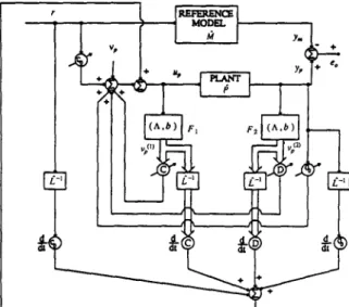
Now the control objective can be stated as follows: under the condition that all the coefficients of the plant transfer function Pu(s) are not known precisely but subject to Assumptions (A1)-(A4), choose a suitable adaptive control law so that, for arbitrary bounded reference input r(t), the overall system is stabilized despite the existence of unmodelled dynamics and bounded output disturbance. Furthermore, the plant output yp will try to follow the model output Ym as closely as possible. Here, the basic controller structure is chosen to be the one in Narendra and Valavani (1978), corresponding to the case of relative degree two. As shown in Fig. 1, the dynamical compensator blocks F1 and F2 are identical single-input, ( n - 1 ) - o u t p u t systems described by transfer functions:

1(:)

e,(s)

..._

(4)

s n 2

The monic characteristic polynomial /~(s) is chosen such that A(s) = nm(S)f-,(S ) where L(s) is

,. ~ + e,

FIG. 1. Structure of model reference adaptive controller.

the one in Assumption (A5). There are a total of 2n parameters to be tuned for the controller due to lack of precise knowledge of Ftp(S) and ap(s). The parameters C e R "-1 in the precompensator block serve to locate the closed loop plant zeros, while D e R n-1 and d 0 e R in the postcompensator block assign the closed loop plant poles. The parameter Co e R then adjusts the overall gain of the closed loop plant. The parameter vector 0 is thus defined as:

O r = [Co, C r, do, D r l r. (5) Refer to the previous problem statement, it can now be restated as how to synthesize the control input up and on-line update the parameter vector 0 so that the aforementioned objective can be met. In other words, a suitable control law and a parameter adaptation law will have to be devised to achieve the purpose. These will be investi- gated in the following sections.

3. PRELIMINARIES

The control scheme to be presented here is an outgrowth of the one in Fu (1991) which only deals with SISO plants with relative degree one. Define the signal vectors w and • :R+---~ R ~ as:

, * =

>

\ @)

/

Note that for any differentiable function hi(-) :R+ =-) R and measurable function h2(') :R+ --> R,

L(s)(hl(t)f~-l(s)(h2)(t) )

d ~ 1

914 Li-CHEN Fu where £(s) is as given before and we use

£-~(s)(h2)(t) to denote the filtered version of h2(t) with filter £-~(s). Define the plant input up

a s :

up = ( 0 ~ + 0 r £ - ~ ( s ) ( ~ ) ) + v~, (8)

which is an implementable input signal once 0 (gives a suitable parameter adaptation law) and vp are specified and from equation (7) is, in fact, equivalent to the following:

u. = L(s)(OrL-~(s)(Ce)) + v,. (9) Note that Vp is an additional input to be given later. It can be shown from Narendra and Valavani (1978) that there exist unique constant parameters 0* • R 2" such that, in the absence of

A/~I(S), AIP2(S), ¢0,

and with Vp = 0 in equations (8) and (9), the transfer function of the plant plus the controller equals that of the model, hT/(s), when 0 - 0 " . This result also directly follows from Narendra and Valavani (1978) since

£(s)(O*r£-'(s)(~)) =- 0*rff. (10) This, in turn, implies that in the ideal case with

v p = 0

yp = P(s)(O*rw) = f.l(s)(r) = Ym" (11) NOW let q~=: 0 - 0* denote the parameter error vector, and ~=:/~-l(s)(ff) and ~ = : £-I(s)(w) denote the filtered version of ff and w, respectively through L-~(s). Then, it can be verified that with the choice of Up in equation (9), yp = P(s)(1 + I~AP~(s))(up) + #AP2(s)(up) = P ( s ) ( O * ~ ) +

P(~)(L(s)(C~) + v~)

+ U(P(s)AP~(s) +

a~(s))(u~)

=Ym + ~ hT/(s)(L(s)(~Pr~) + v,) 1 ^ T ~ + ~oM(S)(D * Fz(s) + d~)(¢o) + # ( l + ~o ~4(s)(D*Tpz(s) + d~) ) × (P(s)APa(s) + APz(s))(up). (12) Denote eo = y p - Ym, then equation (12) can be written as:

= ~OJ~(S)E-~(S)(I~)T~ -I-

/ ~ - I ( s ) ( V R ) + n 0 "3!-

eo #qi),

(13) where

~lo = £-~(s )( O * rPz(s ) + d~')(¢o) = A,0(s)(¢o), (14) and

(

1

)

~, = M - ~ ( s ) + w (D*~P~(s) + d~,)

CO

x (P(s)aP,(s) + AP~(s))L-~(s)(~,,) = £,,(s)L-'(s)(Up). (15)

Here, it can be easily verified that An,(s) and A,o(s ) are stable proper and strictly proper transfer functions, respectively. Since we have assumed

I~ol-<-o,

equation (14) will imply that Irtol<-btp for some b o > 0 . Note that from Assumptions (A4)-(A5), a state space repre- sentation of the error system given by equations (13)-(15) can be readily obtained as:

= Ame + bm(cpr~ + £-'(s)(Vp) + rh, + #0~),

eo = c~e, (16)

and

rli = c~x~ + d~L-'(Up), (17) where

(Am, bin, Cm)

and (A~, be, c¢, de) are

1 ~ ^

minimal realizations of ~om(s)L(s) and /~,,(s), respectively. In particular, A,~ and A¢ are all Hurwitz matrices.

4. A D A P T I V E C O N T R O L L E R D E S I G N

In the previous section, in order to realize the input signal up in equation (8), the time derivative of 0, namely, 0, and the additional signal Vp have to be specified. The former is given by the parameter adaptation law whereas the latter is given by the control law.

Define e0 = eo + ~o = Yp-Ym and consider the modified gradient parameter adaptation law:

0 = ~ = - r ( ~ o ~ + ~o),

I

0(

a = Oo I_~01_ 1 t ( 1 + 1~12 ) O 0 / I~Oo(1 +

I~12)

if 101 < 0o (18) if 0 o - < [01 < 2 0 o if 101 >- 20o, where

I'1

denotes the Euclidian vector norm, F(>0) is the adaptation gain matrix, and o0(>0),

00(---10"1)

are some design parameters. Such an adaptation law is reminiscent of the one in Ioannou and Tsakalis (1986).

Given equations (8) and (18), in the rest of this section, focus will be placed on the choice of Vp so that the overall system is guaranteed to be globally stable and the tracking error is ensured to converge to a residual set whose size is a simple function of # and p while they are small. Let vp be constructed as follows: for some

New robust MRAC using VSD 915 sufficiently small At(>O) and s(>O),

vp = @@&(I& +f(&J &Cl)

+ it (f(W)) --f&0 -

AW)48),

(19) where I&] L E f&J =

Pal < 6

(20)

with { +1 x>o sgn (x) = 0 x=0, ₍₂₁₎ -1 x<o

and n(.):R++R+ is some properly chosen differentiable function.

Remarks.

(1) The function f(&) given in equation (20) in general is not a differentiable function. How- ever, if we can show that f(&J, is, in fact, a piecewise differentiable function, then the signal vp in equation (19) can be re-expressed as:

i-l(WJ

=f@o)&I)

+ A(&>,

where A(&,) satisfies (Fu, 1992)

(22)

P(%)l +llhtllm

+ ~d(zlln,ll- + i ll~&llm + n).

(23)

whenever max (l&,(t)], ]8,(t - At)]) < E for some y1 10, whereas A(&) = s’(t) with c’(t) denoting an exponentially decaying signal (we hereafter abuse the notation s’(t) to denote all the suitably defined exponentially decaying signals) whenever min (l&,(t)], It?,(t - At)]) > E. Suppose that all the signals inside the closed loop system are uniformly bounded, then, it is easily seen that there exists 6 > 0 such that ]A(&,(t))] I 8At for all tr 0 when At is small. Thus, in general the smaller At is, the smaller A(&,) will be. Now with equation (22) the error system in equation (16) can be more concisely expressed as:

2 =&e + b,($‘~

+f(4Ml&

+ A(b) +

vo + CLVi), (24)

e. = cze.

(2) Seemingly, the implementation of vp in

equation (19) will require differentiation of the signal ;IG(.). However, later in the sequel we will explicitly specify the function n(m) (and, in turn,

d -~(a)

dt > so that no explicit differentiation is ever required.

This adaptive controller will first be

investigated in the ideal case where Api = A&(s) = co = 0. The general (non-ideal) case will be treated in Section 5. Therefore, 3, = e, and E = 5 so that the equation (16) can be concisely rewritten as:

t =&e + b,(#? + t-‘(W,)), e. = cfe.

(25)

To study the stability property of the overall adaptive system, Lyapunov analysis is adopted here, i.e. to construct a function V(e, @) as follows:

V(e, #) = teTP,e + f$‘r-‘& ₍₂₆₎

and to evaluate its time derivative: v(e, @) = $eT(AzP, + P=A,)e

+ eTP,b,(qjTc + i-l(s)(~~)) - e,$‘E - ~J@~B, ₍₂₇₎

where P,(>O) satisfies the following properties:

-(AzP, + P,A,) = 2Q,(>O) and P,b, = c,, (28)

due to, the SPR property of the transfer function M(s),!@) in Assumption (A5). In particular, there exist pel, pe2 > 0 and qel, qc2 > 0 such that

pclI -( P, ‘pc21 and qelZ 5 Q, 5 qe21.

Now we are ready to state our main results on the stability as well as the tracking properties of the ideal adaptive system in the foliowing theorem.

Theorem 1. (Global stability and output

trucking.) Consider the previous problem set-up and choose n((f]) as follows:

IElrh

151 <h,

(29)

where & ~0, /12>0, and h is a very small positive number. Then all signals inside the closed loop system are uniformly bounded, i.e. e(e) EL”,, w(e) E L?, and 0(m) EL?, and the size of the residual set of e, is a class K function of E provided that At is sufficiently small. Further- more, if /3i and p2 are chosen large enough, then the residual set is exactly the interval [--E, E], and the set-convergence rate is at least linear in time.

Remark. It can be verified that ~(151) given in equation (29) is indeed a differentiable function

916 LI-CHEN Fu d

and ~ z~(-) is actually implemented as:

d zr(l~l) =

f l l - ~ l ( a ~ - w )

I~l---h

fll--ff(a~-w)

I~1 < h . Furthermore, ~r(l~l) satisfies where fl~ = (ill h + f12). \ 2 (30) (31)

Proof of Theorem

4.1. First, we will show that all signals inside the closed loop system belong to the extended L~ space (Vidyasagar, 1978),

2 n

i.e. e(.)eL$~, w(.) e L®,, and 0 ( . ) • L2~ by investigating the time derivative of the function

V(e, ep).

This investigation will proceed via a contradiction argument, i.e. there exists T > 0 such that some signal inside the system becomes unbounded at t = T. But this presumption implies that all signals remain bounded for all t e [0, T) so that from equations (20) and (25)

f(eo(t))

is indeed a piecewise differentiable function for all t • [0, T). From the previous remark (1) in the beginning of this section, we can readily conclude that the system given in equation (25) is actually equivalent to the following system over that time interval.

= Ame + bm(~pr~

+f(e0):t(l~l) + A(e0)),

eo = c~e.

(32)

As a consequence, equation (27) is simplified as:

f'(e, ¢p) = -era~e - odprO + eof(eo)ZC(l~l)

(33) + eoA(eo).

Due to the fact that

o~prO >-0

and the previous remark about A(eo), whenever e0 is bounded away from the interval [ - e , e], equation (33) becomes

f'(e, q~) ~< -q~l lel 2 - leol(fl2-

e'(t)).

(34) Since

e'(t)

decays exponentially in t, ~" in equation (34) will become negative after some time elapses. This implies that eo cannot grow unbounded at t = T and, hence, neither can the parameter error vector ~(t) and the regressor vector

w(t)

due to Lemma A1 and Lemma A2, respectively (see Appendix for Lemmas and their proofs). This, of course, also implies that ~(t) remains bounded on [0, T]. Therefore, by contradiction, all signals inside the closed loop belong to the extended L® space so that equation (33) remains valid for all t - 0 . This further implies that there exist A t 1 > 0 such that

IA(eo)l < 6(t)At for all At • [0, At1] and for some 6(.) • L ~ because of equations (23), (30), (32), Lemma A3, and the small gain theorem (Desoer and Vidyasagar, 1975). However, 6(0 -< 15 for all t->0 if

e(t),

w(t), and q~(t) are all uniformly bounded.

Now, since equation (33) is valid for all t - 0, it is clear that

(/(e, ~))<-- --qel lel ( l e l -

At([Cml-6-(t)))

(35)

\ qel f i '

\

which according to Lemma A1 and Lemma A3 shows that if Iletllo~<l~(>0), then there exist

12('), 13(.)>0

such that

116,11~<12(11)

and

IlV~ll~<13(ll). On the other hand, the latter inequality, in turn, implies that I le,11~-

~/213(ll). Combining these facts along with

Pc1

equation (35), we can easily see that if we choose At2 to be m i n ( A t l , l o ( ~ ) ) where

le(0)l

lo = , then there exists sufficiently large l~ 11

so that, for all

t >- O,

V(t) <-

13(loll )

<--/3(/1) and, hence, Ile, ll~-<

~zt3£o~tl)

< ll. Consequently, e(.) e L~ and ~ ( . ) • L~, which, in turn, implies that ~ ( . ) • L~ as a result of Lemma A3. From the proof of Lemma A2, it can be verified that w(.) e L ~ as well.

To show the size of the residual set is a class K function of e, further investigation of equation (34) has to be taken. Assume that initially eo stays outside the interval [ - e , e]. Then lel->

E

le01> and hence, after some time t~ > 0

Icml Ic.,I

equation (34) can be rewritten as:

_ qel 2

l?(e, q~)-< icml2 leol - le01 (f12-

e'(t))

< [ qel e2 flze)

- - \ i - ~ +½ t >-- t~, (36) which implies that V is strictly decreasing during this period so that there exists t2 >--t~ such that le0(t2)l-<e. However, once e0 falls into the interval [ - e , e], equation (36) is no longer valid and, hence, V may be increasing so that eo eventually leaves that interval again. To find out the level of magnitude up to which [eol will grow, we augment equation (36) via the use of equation (33) so that

_ ( eel

e2+ fl28)+

x f 2 - i c , , i ~AtV1/2,

f'(e, ~) -< \lcml2 "~ pc1

New robust M R A C using VSD 917 which readily leads to the following conclusion:

leo] ~ .~/--21c.1V1/2<1_~ ( qel

~2+/32E) ' (38)

pe~ - 3At \lcml 2

and, hence, the size of the residual set of eo is indeed a class K function of e. So far, we have concluded the first part of the proof.

In order to show that the residual set is exactly [ - e , e] when /31 and /32 are chosen properly large, we differentiate the output equation (32) so that

eo " eo = eo(cfnAme

+ CT bm( ¢ r~

+ f ( e o ) ~ + A(eo))), (39)

which, whenever leol > e, provides an estimate of the rate of change of leol as:

2dt le°12-<-le01 kp /32- IIc,~tml l e l - 3At

+ kp(fl~ - 141)

I~1),

(40)

where the fact c r b ~ = k e is used. Since ~ and e are uniformly bounded, so long as/31 and/32 can be chosen such that/31---sup I~(t)l and 132 > sup

1

t~tIc

t~tfc

IIc,~,A,,,ll le(t)l + 6At for some finite tic > 0 , equation (40) can be shown to satisfy

l d

dt ]e°12 -< -f13 leol, (41) for some fla > 0 or, equivalently,

d

dt leol -< -2/33, (42) for all t -> ti~. This shows that eo will fall into the interval [ - e , e] at least at the linear rate and will never leave that interval afterwards. This completes the second part of the proof. Q.E.D.

R e m a r k s .

(1) In the theorem, when/31 and /32 a r e chosen properly large, e0 will actually fall into the interval [ - e - A e , e + A e ] for some small Ae > 0 because the statement leoJ > e should, in fact, be replaced by min (le0(t)l, leo(t - At)l) > e. Since At is usually very small, Ae is also kept extremely small. Therefore, in the following we will not differentiate the two testing conditions and will neglect Ae simply for ease of presentation.

(2) Suppose e is very small and /31,/32 are chosen sufficiently large as required in the proof, then the theorem is obviously a drastic improvement of the transient response as well as the tracking performance of the MRAS from

those conventional schemes (Narendra and Valavani, 1978; Narendra et al., 1980; Ioannou and Tsakalis, 1986).

(3) In order to guarantee that fll and f12 are chosen indeed properly large but under the situation that 0* is not known and the state e is not available, some conservative estimates have to be used. From equation (38), V v2 and, hence, 141 are class K functions of e after some time. If e is sufficiently small, fll only needs to be chosen to satisfy fll -> 0o (generally >>e) and the bound on lel can be obtained through an estimation from equations (19) and (25). However, the magnitude of the resulting control input may, thus, become unduly large. A remedy of this situation will be introduced in the following corollary.

(4) In the theorem, in fact, only fl~ needs to be chosen large enough provided the magnitudes of the reference input and, hence, I~1 are bounded away from zero. This fact can be easily seen from equation (40). In other words, in a task of tracking, determination of fll will be crucial to tune the systems performance.

(5) Usually, e is chosen to be very small to guarantee the tracking accuracy. However, under practical digital implementation, e is chosen only reasonably small to prevent excessive switching in the input up due to the finite-step-size numerical integration algorithm.

In the standard adaptive literature, it is well known that the parameter error vector ~ in general does not converge to zero and will do so only when the regressor vector w or, equiv- alently, ~ is persistently exciting (Annaswamy and Narendra, 1988). From the previous results,

/31 has to be chosen to satisfy /31 -> sup I~(t)l in

t~tfr

order to obtain the well-behaved transient response and nice tracking property regardless of the type of tasks, i.e. either stabilization or tracking. Then, it follows from the previous remark (3) that the resulting input may have unacceptably large magnitude to meet that requirement. However, alleviation of such a situation may be attained if Iq~(t)l does converge to a fairly small sized interval asymptotically. The following corollary will state the condition under which this is true.

Corollary. ( E c o n o m i c a l control input d u e to P E

condition.) Consider the previous problem in

Theorem 1 with the same hypotheses. If, furthermore, w is persistently exciting and min I~(t)l I> m~ > 0, then the level of magnitude

t

of fll to ensure the results of Theorem 1 is a class K function of both e and At.

918 LI-CHEN Fu

By applying an argument similar to that in Ioannou and Sun (1990) and equation (40), previous remark (4), we can show that the above corollary is valid (Fu, 1992).

It is also a well-known fact in the adaptive literature that the convergence of the parameter error vector q~ becomes slow when the order of the plant increases. The consequence of such slow convergence is, then, that ty~ after which equation (41) is satisfied will be large and, hence, that the convergence of eo will be slowed down as well. A remedy of this is to forsake the parameter adaptation process and fix 0 at the best estimates of 0* that one can get and adopt the same control law. The following corollary will summarize the resulting property.

Corollary 2. (Fast output convergence without parameter adaptation.) Consider the same problem in Corollary 1 but fix 0 at the best estimates of 0* that one can get. Then all the results in Theorem 1 will remain valid provided

fl, >_ lc~l = lO - O*l .

The proof is quite straightforward if we replace the Lyapunov function V(e, ep) by V(e),

i.e.

V(e) = ½erp, e, (43)

and hence, is omitted here.

Remark. Usually, if the magnitude of the control input is severely constrained, then Corollary 1 will suffice to solve the control problem and incidentally meet the control limitation. However, the slow convergence of the output error may not be desirable due to the limited rate of convergence of the parameter errors q~. Under this circumstance, a remedy is to use some prior information about 0* such as the knowledge of 0min, 0ma x C R 2n where 0m~,- 0 " ~ 0 . . . . and, then, apply the mechanism of Corollary 2. As a result, both economical input design and fast output convergence are achieved simultaneously presuming the size of the interval

[0min, 0max] is much smaller than 0o.

5. ROBUSTNESS TO U N M O D E L L E D DYNAMICS AND O U T P U T DISTURBANCES

In this section, we will examine the robustness property of the adaptive controller in the non-ideal case where A/~l(S), A~'z(s), and ¢o are present. Recall that the error system in this case is given by equations (16)-(17), and the stability of the overall adaptive system will now require the uniform boundedness of x¢ in addition to that of e, w, and 0. Similar to the previous analysis, we first investigate whether all signals

belong to the extended L~ space. Therefore, we assume that there exists finite T > 0 such that some signal grows unbounded at t = T and, hence, for all t e [ 0 , T) the system given by equations (16)-(17) can be rewritten in the following form:

= A ~ e + brn(~bT~ + f(~o)Z -t- 77o

+/trh + A(@o)), (44)

&, = C~m e + ~o = eo + ~o,

~ = A:xc + bc(Or~ + f(~o):r(l~l) + A(~o)), (45)

r h = cffx~ + d¢(Or~ + f(~o)~(l~l) + A(~o)). Construct a function similar to that in (26) as follows:

V(e, (p, x¢) = ½ eTpee + ½ ~pTF-I(p + ½ I~¢~P¢x~,

(46) where P~(>0) satisfies

-(A~P~ + P;A¢) = 2Q~(>0), (47) and differentiate it along the solution trajectories of equations (18), (44)-(45) to obtain the following:

I}" = --(eTae e + p.x~Q~x; + a~pro)

+ {eof(~o)n + eo#(C~X~ + d~(Or~ + f ( ~ o ) n + A(~o))) + eor/o + eoA(~o)}

- (¢o(pT~ -- Izx~P¢b¢(Or~ + f(~,,):r + A(~o))),

(48)

which is to be examined under the circumstance where [~ol>e. Let p ; l , p ~ 2 > 0 and q¢1, q¢2 : > 0 be such that pcl<P¢<<-p¢21 and q¢~l<-Q~<- q;21.

Substitution of equations (20) and (29) into (48) readily leads to the following:

t}" < -- (qe, lel 2 + #q¢, Ix~l z + aq ~rO)

- I~01 {((1 - t~kl)/~,) I~1

+ ((1 - ~kt)132 - I~01 - (1 + t ~ k O E ' ( t ) ) }

+ t~(k3 lel Ix~l + k 4 ( ~ + 101) Ix~l I~1 + k2 101 lel I~1 + ka(13z + e ' ( t ) ) Ix~l) + I~01 {((1 + # k O f l l + (10l + 00))I~1

+ ((1 +/~k~)/3z + Irtol + (1 + I~kOe'(t))},

(49) where kl = Id¢[, kz = Ic,,I Idol, k3 = ICml IC~[, and k4= IP¢bc]. It can be verified (Fu, 1992) that there exist/~2, Pl > 0 such that for all/z e [0,/~2], for all p e [0, pl], and for some ta -> 0

f" -< - (~,a lel 2 + t~'~cl Ix~l 2) + ks/~ Ixcl

+ (k6/~ ~3

I~1 =

+

kvp

I~1

+ k8p), (50) for some q~l, q¢a, ki ~> 0, i = 5, 6, 7, 8, after

t>-q when O(t) turns out to be uniformly bounded in t, i.e. there exists 0m~x > 0 such that

New robust M R A C using VSD 919 [0(t)l ~ 0m~x for all t • [0, T), but

9 -< - (O~ [el 2 +/~Oc~ IX¢l[ 2 + al ItPl 2) + ks/~ [x~l

+ { -- (O'2 11~)12 -- k9~12/3 - ~) 1~] 2

+ k,op

[~[ +

ksp},

(51) for some

al, az, kg,

k i n > 0 when [0(t)l grows gradually unbounded so that there exists

Ot

(-->30O) and

tL

(--0), to be determined later, such that 10(tc)[-> 0c. However, later we will show that the latter case will never occur.

Now, an upper bound and a lower bound on V in equation (46) can be estimated as:

P~--![el2+l'tP¢'2

~

X¢[2

+ ~ [~b[2~ V(e, t~, x¢)

~P¢2 ~ 12 g2

-2<P~--A2[e[2+-~ ~'¢' + ~ - I~12. (52) Let /~3=min(/~l, #z), where /A 1 is given in Lemma A3 in the Appendix. Then, in the case where

[O(t)l<-Om~x

for all t • [ 0 , T), we have

II~,ll~ ~ tl'6 Ile, ll~ + ~7,

where &6 = ~ 6

Ic,,I,

for all

/~ e [0,/~3] as a result of L e m m a A4. Thus, by adding al I~l ~ to the first bracket and Ol(0m,x + 0o) 2 to the second bracket on the right hand side of equation (50), we readily arrive at the following expression:

(Z ~ -- kll V + k12~l/2V 1/2

+ (k6/A2/3 I~1 = + k7o I~1 + k13)

<- - k , i V +

(gl(~) IIV, II~

+ g2(~, p) II Ell& '2 + g3(~, p)),

(53)

for some k s > 0 , i = 11, 12, 13, and for some positive functions K~(#), K2(/z,

p),

K3(IA , p ) ,

where above all K~(/z) is a class K function of/t. On the other hand, in the case where 10(t)l -> 0L -> 300 when t = tL, equation (51) can be expressed as:

~" -~ - k l l

V "k kl21,tl/2v 1/2

+ k,op

I~1

+

ksp},

(54) for all

t • [tL, T).

Now we are ready to state the robustness property of the previously proposed scheme against unmodelled dynamics and output disturbance.

Theorem 2. (Robustness property.)

Given the system considered in Theorem 1 but in the non-ideal case, satisfying Assumptions ( A 1 ) -

(A6). Then, there exist /~*> 0 and p * > 0 such that, for all # e [0,/~*] and p e [0, p*], all signals inside the closed loop system remain uniformly bounded in t provided that At is sufficiently small. Furthermore, the output error e0 will converge to a residual set whose size can be written as an explicit class K function of /~, p, and e provided the control parameters fl~ and

f12

are chosen properly large.

Proof of Theorem

2. Let us first assume that eo grows unbounded at some finite time t = T and, hence, ~o is bounded away from the interval [ - e , el. Under this circumstance, the proof will proceed in two directions, namely, one is to assume

O(t)

is uniformly bounded, i.e. [0(t)[-<

0ma x for all t • [0, T), and the other is to assume

that

O(t)

grow also unbounded so that [0(t)[ -> 0 t -- 300 at t = t L ( < T ) .

In the first direction, the Lyapunov function V has to satisfy the dynamic constraint given by equation (53). Thus, using Bellman-Gronwall lemma, V can be shown to satisfy the following algebraic constraints:

v ( t ) <_ liV, ll~ 1

-<~-~n

(KI(/~)

IIEII= + g2(u, p) IIEIIU

+ K3(~, o)) + e'(t).

(55)

Since KI(/~) is a class K function of /~, there exists /~*, satisfying 0_</~*_</~3, such that

k~lKl(l~ *)

< 1 and, hence,

V(t) <-

IIEII~

(k~'K2 + V(kfilK~ +

4(1 -

klllgl)(k~llg3 --~

,E

')

4(1 -

k ~l~ K1) 2

(56) so long as g • [0,/~*}. Whereas in the second direction where

O(t)

grows unbounded, the dynamic constraint on V becomes equation (54). Now let p*---pa as defined before. Then, it can be verified that, if 0L is defined to be

0L--

+°*'2 20o, 30o), (57,

v

then, for all/~ • [0,/a*] and p • [0,

p*],

equation (54) can be put into an equivalent form:

(/<: - k l l V +

k12t~l12V 1/2 + k14,

(58) for

some k14>0 ,

which readily leads to the following result:

V(t) <--

IIEII~

-< ]((kfilk12/~ 1/2 +

~/(kulka2)21~ +

4k~~lkls) 2. (59) From equations (56) and (59), it is clear that eo,

920 LI-CHEN Fu

in fact, can not escape in finite time t = T and, hence, it belongs to the extended L~ space. This again immediately implies that t~(.)e L2~ and ~(-)eL~'~ from L e m m a A1 and L e m m a A2, respectively. In consequence, the expression of the overall system given by equations (44)-(45) is, then, valid for all t -> 0.

Now, if one further evaluates the derivative of V when 1001 < ~, then it can be verified (Fu, 1992) that, though k12, kl,, K2, and K 3 will have dependence on t and At, they are uniformly bounded provided all the signals e, 9, w, and x~ are uniformly bounded for all t-> 0. Therefore, using the argument in the proof of Theorem 1, it can be easily seen that for sufficiently small At all the aforementioned properties remain valid.

To show the size of the residual set of eo is a class K function of/z, p, and e, we differentiate

e~

the signal ~- in the following as:

eoeo = eo(cf,,Ame

+ kp(~r~

+ f ( e o ) ~ + m ( e o ) -4- ~'~(,--I- 1 . ~ O i ) ) , ( 6 0 ) so that when I~ol > e, we have

l d

2 dt le°12 -< - leol((kpfl2 - IIc~nA,, II lel - kpe'(t)) + kp(fll - Idpl) I~1)

+ G leol ( G P + Irl~l/~) + 2kpp~(l~l), (61) where we use the fact that eo sgn (~o) >-- leol- 2p in the above derivation. Suppose now the control parameters fl~ and 32 are chosen such that for all t >-- ti~, for some finite tr~ - O,

fll -> max I~(t)l,

,~,,, (62)

1

f 1 2 : > tm>at X - IIc,~tmll le(t)l + 8At,

t-t~.~ kp

as required in Theorem 1, then after some re-assignment of notation, equation (61) can be expressed as:

l d

dt le°12 -< -/~3 leol + g4(N, p), (63) where

g 4 ( ~ , P) = kp ICm[ Ile, G (bpp "4" Ilrl,,G)

+ 2kpp II ~,11~. (64) Obviously, K4(0, p) = O ( p ) and K4(/z, 0) = O(/~). Finally, since I~ol > leol - P, whenever leol > P + e, we have 10ol >- e and, hence, equation (63) can be concluded. This implies that eo will eventually converge into a residual set whose size is a class K function of/u, p, and e. This completes the proof. Q . E . D .

6. NUMERICAL SIMULATION EXAMPLES In this section, we will illustrate the effectiveness of the proposed new M R A C scheme by performing the following computer simulation example.

Consider a plant described by

po( ) =

2

(s + 1)(s - 3) (1 + /.t API(S)) + /.t A J62(s), (65) where ]

aA(s) --

s + 1 2 ' A/52(s) = 2 s + 1 0 ' and the reference model is given by

(66)

1

~ z x

(67)

m r s ) - (s + 2)(s + 3)"

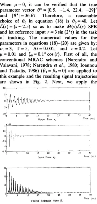
When /~ = 0, it can be verified that the true parameter vector 0* = [0.5, - 1 . 4 , 22.4, -29] r and 10"1 = 36.67. Therefore, a reasonable choice of 0o in equation (18) is 0o = 40. Let £ ( s ) = (s + 2 . 5 ) so as to make lfl(s)f_.(s) SPR and let reference input r = 3 sin (2*0 in the task of tracking. The numerical values for the parameters in equations (18)-(20) are given by: Oo=3, F = 5 , A t = 0 . 0 0 1 , and e = 0 . 2 . Let # = 0 . 0 1 and ~0 = 0.1* cos (t). First of all, the conventional M R A C schemes (Narendra and Valavani, 1978; Narendra et al., 1980; Ioannou and Tsakalis, 1986) (ill = fiE = 0) are applied to this example and the resulting signal trajectories are shown in Fig. 2. Next, we apply the

5 0

15 20 25 30 35 40 Output E~or e o Time (see) 0 5 lO I x104

°"t 11

50 5 1'0 15 20 25 30 35 Input Force up 40 l'ime (sec) 3O 10 0 0 5 10 15 20 25 30 Filtered Regressor Norm I~1 FIG. 2. Conventional scheme.

3;- --%o Time (see)

New robust MRAC using VSD 921

1: t

0.5 0 1 2 8OO0 -2 _{o ~ ;} 3 4 5 6 7 8 9 10

Output Error ~o Time (sec)

Time (sec) Input Force up 0 . . . ----'" . . . "" eo -0-~ ' ' ' 0 1 2 3 4 5 6 7 8 Output Error ~o 200 -2 ; lO Time (see) 0 1 2 3 4 5 6 7 8 9 10 Time (sec) Input Force up i . . . . 0 _{0 1 2 3 4 5 6 7 8 9 10} Time (see)

Filtered Regress~¢ Norm I~l FIG. 3. r = 3 sin (2*t), /~l = 40, /32 = 1. 2 . . . . . . . . . 1 . 5 1 0.5 0 0 1 2 3 4 5 6 7 8 9 10 Time (sex) Filtered Regressor Norm I~1

FIG. 5. #mi. = [0.1, - 2 , 22, - 3 0 ] r a n d 0,..x = [0.9, - 1 , 23, - 28] r, 0 = 0mi. a n d r = 3 sin ( 2 ° 0 .

proposed scheme in different situations: (i) Suppose the knowledge about 0* is only the upper bound of its norm, i.e. 0o. Then, we choose fl1=40 and let f12= 1, following Remarks (3) and (4) after the proof of Theorem 1 in Section 4. Figure 3 illustrates the resulting signal trajectories. (ii) Suppose the reference input is enriched so that r = 3 s i n ( 2 * t ) + 2 sin (4*0. Then, fll can be greatly reduced so that fl~ = 2 but /32 remains the same, based on the result of Corollary 1. The resulting signal

1.5 . . . .

O.5

4)

0 1 2 3 4 5 6 7 8 9 10

Output Error #o Time (sec)

1

-100

0 1 2 3 4 5 6 7 8 9 10 Time (sec)

Input Force up

trajectories are provided in Fig. 4. (ii) Suppose the interval in which 0* lies is [0r.i., 0r.ax], where 0rain = [0.1, - 2 , 22, -30] r and 0max = [0.9, - 1 , 23, -28] r. Then, from the remark after Corollary 2, we let 0 = 0min and choose fll = 3, since 10max- 0mi, I = 2.58, but let f12 still remain the same. In Fig. 5, the resulting signal trajectories are provided. (iv) Finally, just to show the drastic improvement of both the transient behavior and the tracking performance of the closed loop system by adding small

0 .- . . . . - . . .

-0,5 e°

0 1 2 3 4 5 6 7 8 9 10

Output Errs" to Time (sec)

4O 20

-2

0 1 2 3 4 5 6 7 8 9 10

Input Force up Time (sec)

2 . . . .

0.

1 2 3 4 5 6 7 8 9 10 Filtered Regressor Norm 1~[ Time (sec)

FIG. 4. r = 3 sin (2*t) + 2 sin ( 4 * 0 , ~1 = 2, ~2 = 1.

0.5

0

0 1 2 3 4 5 6 7 8 9 10

Filtered Regressor Norm [~] Time (see)

922 LI-CHEN Fv

IL50 -0.5 -1

0 5 10 15 20 25 30

Input Force up of Proposed Scheme Time (sec)

i!llJlll

!ll Ii

Time (sec) Input Force u e of Conventional Scheme

FIG. 7. Comparison between the conventional scheme and the proposed scheme.

quantity of Vp into up as given in (3.3), we let fll = 0 and f 1 2 = 2. The simulated signal trajec- tories are illustrated in Fig. 6, which seem to be much better behaved than those in Fig. 2. For interesting comparison, a close-up of the time evolutions of the input force up applied in the conventional scheme and that in the current scheme in situation (iv) in Fig. 7 suggests that the steady state Up of the proposed scheme has smaller magnitude and evolves smoother with time than that of Up in the conventional schemes.

7. CONCLUSIONS

The paper presented a new robust MRAC scheme for SISO plants with relative degree two, which incorporated the similar VSD concept in Fu (1991) and was based on the modified MRAC scheme proposed in Narendra and Valavani (1978) particularly for the case with relative degree two. No assumption of PE condition is needed here in order to ensure the global stability of the overall system, in a way similar to o- (Ioannou and Kokotovic, 1984b; Ioannou, 1986; Ioannou and Tsakalis, 1986) and el- modification (Narendra and Annaswamy, 1987). Since the controller is a continuous one in nature, no Filippov's notion is used and hence, the input force is generally kept with a moderate level of magnitude and usually evolves with smoother time trajectory. The striking features of the proposed controller are the drastic improvement of the transient behavior and the tracking performance from the conventional schemes (Narendra and Valavani, 1978; Narendra et al., 1980; Ioannou and Tsakalis, 1986) which are clearly demonstrated in the simulation example.

In the proposed scheme, both parameter update process and the input interaction contributed to the stabilization of the overall system. Due to this sharing of load between two

mechanisms in handling the parameter uncer- tainties, the magnitude of the resulting input force has been greatly reduced as opposed to those observed in Narendra and Valavani (1978), Narendra et aL (1980) or Fu (1991). Furthermore, if the reference input satisfies the PE condition or if the prior knowledge about the neighborhood of the system parameters is available, then the input magnitude can be reduced further or even the rate of convergence can be increased as well. In the presence of mild unmodelled dynamics and bounded output disturbance the proposed scheme was shown to be robust and the resulting tracking errors will fall into a residual set whose size has been related directly to the size of unmodelled dynamics and of output disturbances.

REFERENCES

Ambrosino, G., G. Celentano and F. Garofalo (1984). Variable structure model reference adaptive control systems. Int. J. Control, 39, 1339-1349.

Annaswamy, A. M. and K. S. Narendra (1988). Stable

Adaptive Systems. Prentice-Hall, Englewood Cliffs, NJ. Anderson, B. D. O., R. R. Bitmead, C. R. Johnson, P. V.

Kokotovic, R. L. Kosut, I. M. Y. Mareels, L. Praly and B.

D. Riedle (1986). Stability of Adaptive Systems, Passivity,

and Averaging and Analysis. MIT Press, Cambridge, MA. Astr6m, K. J. (1935). Interaction between excitation and

unmodelled dynamics. IEEE Trans. on Aut. Control,

AC-30, 889-891.

Bodson, M. (1986). Stability, convergence, and robustness of adaptive systems, Ph.D. Dissertation, University of California, Berkeley.

Bodson, M. and S. S. Sastry (1984). Small signal I/O stability of nonlinear control systems: application to the robustness of a MRAC scheme, Memorandum, No. UCB/ERL M84/70, Electronics Research Laboratory, University of California, Berkeley.

Bodson, M. and S. S. Sastry (1989). Adaptive Control:

Stability, Convergence, and Robustness. Prentice-Hall, Englewood Cliffs, NJ.

Chert, Z. J. and P. A. Cook (1984). Robustness of model reference adaptive control systems with unmodelled dynamics. Int. J. Control, 39, 201-214.

Desoer, C. A. and M. Vidyasagar (1975). Feedback Systems:

Input-output Properties. Academic Press, New York.

Egardt, B. (1979). Stability of Adaptive Controllers.

Springer-Verlag, New York.

Egardt, B. (1980). Stability analysis of adaptive control

systems with disturbances. Proc. JACC, San Francisco,

CA.

Fu, L. C. (1991). A new approach to robust model reference adaptive control for a class of plants, lnt. J. Control, 53, 1359-1375.

Fu, L. C. (1992). A new robust model reference adaptive control using variable structure design for plants with relative degree two. Technical Report, NTUEE 92-1, Department of Electrical Engineering, National Taiwan University, Taipei, Taiwan, R.O.C.

Fu, L. C. and S. S. Sastry (1987a). Frequency domain analysis and synthesis techniques for adaptive systems,

Memorandum, No. U C B / E R L M87/58, Electronics

Research Laboratory, University of California, Berkeley. Fu, L. C. and S. S. Sastry (1987b). Slow drift instability in

model reference adaptive systems--an averaging analysis. Int. J. Control, 45, 503-527.

Hsu, Liu (1990). Variable structure model-reference

New robust MRAC using VSD 923

measurements: the general case. IEEE Tram. Aut.

Control, 35, 1238-1243.

Ioannou, P. A. (1986). Robust adaptive controller with zero

residual tracking errors. 1EEE Trans. Aut. Control,

AC-31, 773-776.

Ioannou, P. A. and P. V. Kokotovic (1984a). Instability analysis and improvement of robustness of adaptive

control. Automatica, 20, 583-594.

Ioannou, P. A. and P. V. Kokotovic, (1984b). Robust

redesign of adaptive control. IEEE Tram. on Aut.

Control. AC-29, 202-211.

Ioannou, P. A. and K. S. Tsakalis (1986). A robust direct

adaptive control. IEEE Tram. Aut. Control, AC-31,

1033-1043.

Ioannou, P. A. and J. Sun (1990). Parameter Convergence

of modified adaptive laws with persistent excitation. Proc.

American Control Conf., pp. 565-566.

Kokotovic, P. V., B. Riedle and L. Praly (1985). On a

stability criterion for continuous slow adaptation. System

and Control Letters, 6) 7-14.

Kosut, R. L. and C. R. Johnson (1984). An input-output

view of robustness in adaptive control. Automatica, 20,

569-581.

Kosut, R. L. and B. Friedlander (1985). Robust adaptive

control: conditions for global stability. IEEE Tram. Aut.

Control, AC-30, 610-624.

Krause, J., M. Athans, S. S. Sastry and L. Valavani (1983).

Robustness studies in adaptive control. Proc. 22nd IEEE

Conf. on Decision and Control.

Kreisselmeier, G. and B. D. O. Anderson (1986). Robust

model reference adaptive control. IEEE Tram. Aut.

Control, AC-31, 127-133.

Kreisselmeier, G. and K. S. Narendra (1982). Stable model reference adaptive control in the presence of bounded

disturbances. IEEE Tram. Aut. Control, AC-27, 1169-

1175.

Narendra, K. S. and L. Valavani (1978). Stable adaptive

controller design-direct control. IEEE Tram. Aut.

Control, AC-23, 570-583.

Narendra, K. S. and A. M. Annaswamy (1987). A new adaptive law for robust adaptation without persistent

excitation. IEEE Tram. Aut. Control, AC-32, 134-145.

Narendra, K. S., Y. H. Lin and L. Valavani (1980). Stable

adaptive controller design, Part II: proof of stability. IEEE

Tram. Aut. Control, AC-25, 440-448.

Ortega, R., L. Praly and Y. Tang (1987). Direct adaptive tuning or robust controllers with guaranteed stability

properties. System and Control Letters, 321-326.

Peterson, B. B. and K. S. Narendra (1982). Bounded error

adaptive control. 1EEE Tram. Aut. Control, AC-27,

1161-1168.

Riedle, B. D. and P. V. Kokotovic (1985). A stability- instability boundary for disturbance-free slow adaptation

and unmodeiled dynamics. IEEE Tram. Aut. Control

AC-30, 1027-1030.

Rohrs, C. E., L. Valavani, M. Athans and G. Stein (1985). Robustness of continuous-time adaptive control algorithm

in the presence of unmodelled dynamics. IEEE Trans.

Aut. Control, AC-30, 881-889.

Sastry, S. S. (1984). Model reference adaptive control:

stability, parameter convergence and robustness. I.M.A.J.

Control, and Inform., 1, 27-66.

Vidyasagar, M. (1978). Nonlinear Systems Analysis.

Prentice-Hall, Englewood Cliffs, NJ.

APPENDIX Lemmas and proofs

Lemma A1. Consider the parameter update law given by equation (18). Then, there exist oq, o~2 > 0 such that

11¢,11~ -< 06 [Igo, ll~ + a~2. (A.I)

Proof of Lemma A1. With loss of generality, we only need

to consider the case where 101>20o. Therefore, equation (18) becomes

0 = -F($o~ + %(1 + I~lz)0). (A.2)

Define a Lyapunov function Vo = ½0rF-~O and, then, take

its time derivative along the solution trajectories of (A.2) to obtain the following:

d

dt Vo = - % 1012 - oo 1012 I~l 2 - #-oOT~

2o0 I~ol 2 ( ~ I~olX 2

<--g-TV.+~Oo-Oo.tot

~ - ~ o )

-< - 2°°g--~ V° +41~012o--~' (A.3)

,~,~ere we use the fact that gll<-I'-l<:gEI for some

gl, g2 >0- Thus, by Bellman-Gronwall lemma, the bound on 0 can be derived as:

10l 2 -< ~ I1~0,11~ + e'(t), (A.4)

'~o-ogl

where e'(t) is due to the stable initial conditions. Let a~ = ~o01 \~/(g2~ 1/2 a n d fiE = mtax e'(t)+ 0 o. Then, it follows that

Ile, ll®<- IlO, II~ + Oo<- oq ll~o, ll~ + a2 . (g.5)

This completes the proof. Q.E.D.

Lemma A2. Consider the problem described in Section 2 and Section 3, satisfying Assumptions (A1)-(A6). Let the adaptive controller be designed according to Section 4. If

L®~ and, hence ~(.) e L~.

%(.) • L ~ , then ~,(.) • z, ^ 2,

Proof of Lemma A2. First of all, from the hypotheses and Lemma A1, we know that ~(.) e L ~ . To show that ~(.) and 2, ~(.) belong to the extended L® space, we assume the contrary, i.e. there exists T > 0 such that [ff'(t)l grow unbounded at t = T, and prove that such an assumption will lead to a contradiction.

Let the compensator blocks F 1 and F 2 be realized by a (n D × ( n 1)

controllable pair (A, b), where A • R - - is Hurwitz

and b • R (n-l), so that ~ ( s ) = ~ ( s ) = ( s l - A)-Ib. Thus we

h a v e

epl)= Av~O + b%,

(A.6) 9p(2) = Avp(2) + b(y v + ¢o),

and, hence, ~i and ~2 will satisfy ~, = A~I + bf-,-l(uv) + e'(t)

= A~, + b(Or~ + L.-'(s)(vp)) + e'(t), (A.7)

~2 = A~2 + bL-t(yv + ~o) + e'(t).

It then follows from (A.7) that

ll~2,11®<-Y2llYp, ll~+y3, for all t • [0, T], (A.8)

for some positive constants )'2 and )% Furthermore, as a result from equations (19), (30)-(31), a bound on £ - I ( v , ) can be estimated as:

+ r, +/~,£-'(s)(N,I) = Y4 I1~,11= + 75 + fl~£-l(s)(l~l), for some y4, Ys>0. Denote f f = ( w ( o , . . . , w ( 2 n ) ) r • R zn and ~ = L-a( i f ) = (~0) . . . ~(z~)) r • R2~- Suppose for some j, l<-j<--2n, wj(t) grows unbounded at t = T . Then, there exists t r ->0 such that wo)(t ) = sgn (wq)(tl)) Iwto(t)l for

9 2 4 L I - C H E N F U all t ~- t: and, hence,

l~q)(t)[ = I(e -m'~)wO)('r) dT --> ~ ' e - ° 0 - ' ) Iw0)(r)[ dz _ ~t/e-aO- r)Wuidl7 dO = e-U~'-° [wf/)(r)[ d r J0 - ]fie -``(' ~)wq)('r) d r

~

tf e a(t--T) - ~o Iwu)(r)l d r >-- L-t(s)(Iw(j)l)(t ) - Y6

for all t • [t:, T], (A.10)

for some )'6 > 0. O n the other hand, if wt/)(t) is b o u n d e d on [0, T], then (A.10) will be even more trivially satisfied. Therefore, with the help of the facts that

I)~l-<~lw~)[ and ~ l ~ o ) l - < ( 2 n ) U 2 1 ~ l , (A,11)

J i

we can readily deduce from (A.10) the following:

£-~(s)(l~'l) -< (2n) vz I~1 + )'7, (m.12)

for some positive constant )'7. Combining (A.9) with (A.12), we thus have

112 '(vp)l-< 94 )I$,11~ + 9~, (A.13) where 94 = )'4 + fll(2n) 1/2 and 95 = Y5 -~- )'7' Finally, by substitution of (A.13) into the estimate of the rate of change of ~t in (A.7), we will have

I~l <- (IIA + bCr(t)[[ + 94) It~,11~ + (llbDr(t)[I + 94) 11~2~11~

+ (Ibdo(t)l + 94)II(L-t(yp + ¢0)),11~

+ {(Ibco(t)l + 9,)11 ( £ ~(r)),ll~ + Ibl ?_~ + le'(t)l} -< o~3 II~,,lt~o + ~r~ IlYmll~ + o<5

for all t ~ [0, T), (A.14)

where

o~ 3 = max (IIA + bCr(t)ll + 94),

t~0

m a x ( 1)

°:4 = (llbDr(t)ll + 9,)72 + (Ibdo(t)l + 94)a , (A.15)

o:5 = max ((Ibco(t)l + 94) [£ l(r)l + (llbDr (t)ll + 94))'3

t~0

+(Ibdo(t)l + 94)(IL 1(¢o)1 + )'~) + le'(t)l + Ibl 95).

Note that in the above derivations we have used the facts that

I1~,11+ -< II(£-t(r)),ll® + I1~,11~

+ II(L-t(yp + ~o))Al~+ ll~2,ll~. (A.16) Apparently, I~l(t)l can not grow u n b o u n d e d at t = T and,

(2) in hence, neither can Iv(p°(t)l due to (A.14). Obviously, vp (A.6) can not grow u n b o u n d e d either. Therefore, the result of the iemma directly follows from the contradiction.

Q . E . D .

Lemma A3. Consider the same problem in L e m m a A2 and

let e0(. ) e L®,. Suppose the adjustable p a r a m e t e r vector O(t) turns out to be uniformly bounded. Then, there exists #t > 0 such that for all/z • [0, #1], ~ will satisfy

11 ~rl[~ --< (x611 eoAl® + or7 for all t-> 0, (A.17) for some re6, o 7 > 0 .

Proof of Lemma A3. L e m m a A2 reveals that all signals

belong to the extended L~ space and, hence, equation (22) becomes valid for all t >-0 owing to the arguments in the beginning of T h e o r e m 1. Then, it can be easily seen that with the above fact (A.13) only needs to be modified slightly into the following:

[ £ - I ( V p ) [ - 94 I1~,t1~ + % IA(~o)l, (m.18)

which now remains valid for all t - 0. This, in turn, implies that (A.14) will be modified accordingly as:

I~ll <: 0(3 II@l,ll~ + oq IlYp, ll® + a5 + &5 IA(0o)l

for all t -> 0, (A. 19)

for some &5.

Furthermore, since P,(s)(Up)=yp, from (A.6), it is clear

that

~2 = / 5 , ( s ) ( ~ , ) + ( s l - A) lb/~ '(~o) + e'(t). (A.20) Define ~o= ( s l - A ) - l b £ - l ( ¢ o ) and recall that P,,(s) = P (s)(1 + #APt(s)) + #APz(s ). Then, it can be derived that

~3 =: ~2 - u a P 2 ( s ) ( ~ , ) - ~o = k ( s ) O + u a b , ( s ) )

x (~1) + e'(t). (A.21)

By Assumption (A1) and ( A 3 ) , / ~ ( s ) is m i n i m u m phase with

relative degree two. Now if we define z(t) = ~ (~1) for

some a o > 0 to be determined later and borrow the results from the proof of L e m m a 3.6.2 in Bodson and Sastry (1989) then we can deduce that

IlNul[~ -< Ilz, tt~ + IIE;IL + 2 II~l, ll~, (A.22) and from (A.19) we can further conclude that

1

I1~1,11~--- "1 2

×

so long as ao is chosen such that 2 o<3 < 1.

a o

On the other hand, ~ ib(s) has a stable inverse from

ao

Assumption (A3) and, hence,

a 2 ^

z = ~ P - I ( s ) ( ~ 3 - e'(t))

- #A/31(s)(z), (A.24)

which implies that there exists #o -> 0 such that

IlzAl~ -< y8 ll~3,ll~ + (y9 + #yao), (A.25)

for all # e [0, #o] and for some appropriate positive constants Y s - Yl0- It can also be shown from (A.21) that

11 ~3tl[~ <: l[ ~2t 11~ + # r l I I I ~ltll® + ( z n + ~713), (A.26) for another set of appropriate positive constants V11 - Y~3. Combining (A.23), (A.25) and (A.26), we can attain the following

~t,ll® -< 1 ()'s II ~ II- + #()'8Yl 0 II ~u

II I1~

+ Y s ( V 1 2 + #)'13) + (5'9 + #Y12)), (A.27) where Y~4 = 1 - 2 o~3 > 0. Now, clearly, there exists #1 -</Zo such that, for all/., e [0,/*1], (A.27) can be rewritten as:

[iNI,[[®-< )'1511~2AI~ + )'16, (A.28)

N e w r o b u s t M R A C u s i n g V S D 9 2 5

from (A.8) that

II~,ll ~ Y2Y15 II(Yw -Ym),ll~

+ max (Y2Y15 IlYm, ll~ + (~/3Y15 "j" Y16)) t~O

= Yt7 Ileo, ll® + Y~8, (A.29)

for some )'17, YlS > 0 . H e n c e , using (A.8) and (A.29) in (A.16), we can conclude that

I,~,ll® < (y2 + Y,7 + 1 ) Ileo, ll®

+ max ((1+)'2)'[YmtJ'® + [£-Z( r+ ~0)]) + (~q + ~'3 + Y~8)

= 0~6 Ileotil~ + 0tT. (A.30)

This concludes out proof.

Lemma A4. Consider the same problem in L e m m a A2 but let eo grow u n b o u n d e d at some finite time t - - T < so. Then, [~(t)l will also become u n b o u n d e d at t = T. Furthermore, if

O(t) remain uniformly b o u n d e d for all t e [0, T), then the result of l . e m m a A3 will hold for all t e [0, T).

Proof of Lemma A4. The fact that e 0 grows u n b o u n d e d at t = T is equivalent to having yp grow u n b o u n d e d at t = T. Recall that

1(i/

v~ 2) = ~ (Yp + ~o), (A.31)

\ s " - U

where .,~(s) is Hurwitz. We claim that to prove the first part 1

of the lemma it suffices to show that ~ ( y p ) grows

unbounded at t = T for all a 0 > 0. T h e reason of the claim is given as follows: Let/~,(s) =/~l(s)/k2(s ) where Al(s ) = 0 has real roots but A2(s ) = 0 only has complex roots. Moreover, let the degree of the polynomial A2(s ) be n 1. Then, by applying the claim successively, it is clear that the signal

A~(s)(s + a~)", (y" +

where x denotes the first element of v~ 2), becomes u n b o u n d e d at t = T. Therefore, by use of the stable filter theory, it follows that x and, hence, [v~2)J become u n b o u n d e d at t = T as well. This, in turn, says that I~[ grows u n b o u n d e d in finite time t = T and, thus, one can deduce from the proof of L e m m a A2 that [~J will also become u n b o u n d e d at that same finite time. Finally, the proof of showing that

1

(s + ao) (yp) indeed grows u n b o u n d e d at t = T will be similar to that given by (A.10) in the proof of L e m m a A2. This completes the first part of the proof.

To show the second part of the lemma, recall in (A.14) that

I~11 ~< oc3115,11® + t~4 IlYp, ll® + 0~5

for all t e [0, T). (A.33)

Consequently, it can be deduced from the proof of L e m m a A3 that its result will remain valid for all t ¢ [0, T). O . E . D .