適用於非對稱網路連線之動態用戶的彈性應用層多點傳播

全文

(1)國立交通大學資訊科學與工程研究所碩士論文. 適用於非對稱網路連線之動態用戶的彈性應用層多點傳播 Resilient Application Layer Multicast Tailored for Dynamic Peers with Asymmetric Connectivity. 研究生：郭宇軒指導教授：邵家健. 副教授. 中華民國九十五年七月.

(2) 適用於非對稱網路連線之動態用戶的彈性應用層多點傳播 Resilient Application Layer Multicast Tailored for Dynamic Peers with Asymmetric Connectivity 研究生：郭宇軒. Student：Yu-Hsuang Guo. 指導教授：邵家健. Advisor：John Kar-Kin Zao. 國立交通大學資訊科學與工程研究所碩士論文. A Thesis Submitted to Institute of Computer Science and Engineering College of Computer Science National Chiao Tung University in partial Fulfillment of the Requirements for the Degree of Master in Computer Science July 2006 Hsinchu, Taiwan, Republic of China. 中華民國九十五年七月.

(3) 適用於非對稱網路連線之動態用戶的彈性應用層多點傳播. 學生：郭宇軒. 指導教授：邵家健. 國立交通大學資訊科學與工程研究所碩士班. 摘. 要. 我們的目的是設計出一個有彈性的應用層多點傳播架構，來提供即時多媒體串流服務。我們主要是針對應用層多點傳播的兩個問題。第一、組成應用層多點傳播的用戶隨時都會動態的加入或離開，因此資料傳輸並不可靠。第二、使用非對稱網路連線的用戶，它們上傳的頻寬遠遠少於下載頻寬，上傳的頻寬不足將會是應用層多點傳播的瓶頸。我們提出三種方法的結合來產生出一個有彈性的應用層多點傳播機制，並且解決上傳頻寬不足的問題。這三種方法是：一、information dispersal algorithm，二、multiple stripes/trees，三、helper。我們增強彈性的方法是藉由保證訂閱戶就算遺失一些封包仍然可以得到完整資料，以及任一條網路連線中斷將不會有訂閱戶收不到任何封包。我們解決上傳頻寬不足的方法是充分利用所有用戶的上傳頻寬，以及藉由 helper 的加入來增加上傳頻寬的總量。我們從模擬實驗中觀察到幾項結果：一、每個訂閱戶的訊息延遲時間是穩定的，而且訂閱戶之間的訊息延遲時間差距很少，二、就算對上傳頻寬不足的非對稱網路連線而言，每條網路連線的平均頻寬消耗是少的，三、結果顯示就算用戶有機率會發生錯誤時，訂閱戶仍然有良好的訊息成功還原率。. i.

(4) Resilient Application Layer Multicast Tailored for Dynamic Peers with Asymmetric Connectivity. Student: Yu-Hsuang Guo. Advisor: John Kar-kin Zao. Institute of Computer Science and Engineering National Chiao Tung University. ABSTRACT. Our purpose is to devise a new application layer multicast scheme to provide real time multimedia streaming service. There are two challenges for application layer multicast that we focus on. First challenge is peers that form the application layer multicast service may dynamically join or leave at any time. Data transmission is not reliable. Second one is peers with asymmetric connectivity that upstream bandwidth is much less than downstream bandwidth. Insufficient upstream bandwidth will be the bottleneck of application layer multicast. We propose the combination of three approaches to provide a resilient application layer multicast mechanism and solve the issue of peers with insufficient upstream bandwidth. The three approaches are: (1) information dispersal algorithm, (2) multiple stripes/trees, (3) helper. We improve resilience by promising subscribers can tolerate some packets loss without losing data completeness and when any link break, none of subscribers can’t receive any packets. We solve the insufficient upstream bandwidth issue by fully utilizing the upstream bandwidth of all peers and increasing the total amount of upstream bandwidth by the participation of helpers. We observe several results from the simulation: (1) the delay of message restoration for each subscriber is stable and the difference of delay between subscribers is small, (2) the average bandwidth consumption of one link is low, even for insufficient upstream bandwidth links, (3) it shows subscribers have good successful probability of message restoration even if peers have failure probability.. ii.

(5) 誌. 謝. 首先我要感謝邵家健老師，整個論文題目、方向、作法都是經由不斷和老師討論，以及老師給予許多建議與指引才有辦法產生，如果沒有老師的協助，我將無法獨力完成；再感謝老師在這兩年的教導，無論是研究方法或是待人處事，真的令我獲益良多。另外感謝林哲民學弟協助撰寫工具程式，令 GT-ITM 產生的網路拓樸可以匯入到 OMNeT++；感謝黃淩軒學弟幫忙分析實驗數據來畫出其中一張數據圖；感謝尤清華協助畫出兩張口試投影片所使用的樹狀結構圖；感謝張哲維學長與我討論技術問題並且提供寶貴建議；最後感謝其它 620 實驗室的成員，包含龔哲正、吳事修、陳奕興、黃為霖、朱書玄、黃國晉、李明龍、劉育志，你們是我最好的伙伴。. iii.

(6) Contents 摘. 要..............................................................................................................................................................I. ABSTRACT .......................................................................................................................................................... II 誌. 謝.......................................................................................................................................................... III. CONTENTS.........................................................................................................................................................IV LIST OF FIGURES........................................................................................................................................... VII LIST OF TABLES ............................................................................................................................................VIII CHAPTER 1 RESEARCH OVERVIEW ............................................................................................................ 1 1.1 PROBLEM STATEMENT ................................................................................................................................. 1 1.1.1 Dynamic Peers ...................................................................................................................................... 1 1.1.2 Asymmetric Connectivity....................................................................................................................... 1 1.2 RESEARCH APPROACH ................................................................................................................................. 2 1.2.1 Definition of Resilience......................................................................................................................... 3 1.2.2 Three Approaches.................................................................................................................................. 3 1.3 OUTLINE OF THESIS ..................................................................................................................................... 4 CHAPTER 2 BACKGROUND ............................................................................................................................ 5 2.1 ARCHITECTURE OF MULTICAST .................................................................................................................. 5 2.2 RELATED WORK ........................................................................................................................................... 6 2.2.1 Multiple Description Coding (MDC) .................................................................................................... 6 2.2.2 Multiple Stripes ..................................................................................................................................... 6 2.2.3 Waypoint................................................................................................................................................ 7 2.2.4 Tree Building Algorithm........................................................................................................................ 7 2.2.5 Enhancement of Resilience ................................................................................................................... 8 CHAPTER 3 PRINCIPLE.................................................................................................................................... 9 3.1 OVERALL SYSTEM ........................................................................................................................................ 9 3.2 INFORMATION DISPERSAL ALGORITHM (IDA) ......................................................................................... 10 3.2.1 Split ..................................................................................................................................................... 10 3.2.2 Restoration.......................................................................................................................................... 12 3.2.3 Efficiency............................................................................................................................................. 12 3.2.4 Advantage ........................................................................................................................................... 13 3.2.5 Influence of n and m............................................................................................................................ 13 iv.

(7) 3.3 MULTIPLE STRIPES/TREES ........................................................................................................................ 14 3.3.1 Combine with IDA............................................................................................................................... 14 3.3.2 Building Disjoint Paths....................................................................................................................... 15 3.3.3 Become Interior Node ......................................................................................................................... 16 3.4 HELPER....................................................................................................................................................... 17 3.4.1 Demand of Helper............................................................................................................................... 17 3.4.2 Find Helper......................................................................................................................................... 17 3.4.3 Restriction of Helper........................................................................................................................... 18 3.4.4 Helper Join ......................................................................................................................................... 19 3.4.5 Enhancement....................................................................................................................................... 20 3.4.6 Difference between Helper and Waypoint ........................................................................................... 21 CHAPTER 4 MECHANISM.............................................................................................................................. 22 4.1 SERVICE STARTUP ...................................................................................................................................... 22 4.1.1 Establish Neighbor Table .................................................................................................................... 22 4.1.2 Source of Service................................................................................................................................. 23 4.1.3 IDA Configuration .............................................................................................................................. 24 4.1.3.1 (n, o, m) IDA.................................................................................................................................................24 4.1.3.2 Apply to Streaming Data.............................................................................................................................25 4.1.3.3 Discussion.....................................................................................................................................................25. 4.2 BEHAVIOR OF PEERS .................................................................................................................................. 26 4.2.1 Architecture of Peer Behavior............................................................................................................. 26 4.2.2 Join ..................................................................................................................................................... 26 4.2.2.1 Randomly Join o Trees................................................................................................................................26 4.2.2.2 Choose Parents ............................................................................................................................................27 4.2.2.3 Cases of Join Accept ....................................................................................................................................28. 4.2.3 Receive and Retransmit....................................................................................................................... 30 4.2.3.1 General Retransmission..............................................................................................................................30 4.2.3.2 Stripe Regeneration.....................................................................................................................................31. 4.2.4 Adjust Number of Joining Trees .......................................................................................................... 32 4.2.4.1 Foundation ...................................................................................................................................................32 4.2.4.2 Increase and Decrease .................................................................................................................................33 4.2.4.3 Priority of Joining Tree Selection...............................................................................................................34. 4.2.5 Leave................................................................................................................................................... 34 CHAPTER 5 PERFORMANCE ANALYSIS.................................................................................................... 36 5.1 PURPOSE ..................................................................................................................................................... 36 5.2 SYSTEM CONFIGURATION .......................................................................................................................... 36 5.2.1 Network Topology ............................................................................................................................... 36. v.

(8) 5.2.2 Link and Traffic Condition .................................................................................................................. 37 5.2.3 Trickle Setup........................................................................................................................................ 38 5.2.4 Streaming Data Setup.......................................................................................................................... 39 5.3 EXPERIMENT .............................................................................................................................................. 39 5.3.1 Metrics ................................................................................................................................................ 39 5.3.2 Procedure............................................................................................................................................ 40 5.4 RESULTS AND ANALYSIS ............................................................................................................................. 41 5.4.1 Restoration Delay and Stripe Delay.................................................................................................... 42 5.4.1.1 Delay for Individual Subscriber .................................................................................................................42 5.4.1.2 Delay for Trickle ..........................................................................................................................................43 5.4.1.3 Relative Delay Penalty (RDP).....................................................................................................................46. 5.4.2 Link Stress ........................................................................................................................................... 47 5.4.3 Probability of Success Restoration ..................................................................................................... 48 CHAPTER 6 CONCLUSION............................................................................................................................. 50 6.1 ACCOMPLISHMENT .................................................................................................................................... 50 6.2 FUTURE WORK ........................................................................................................................................... 51 REFERENCE ...................................................................................................................................................... 53 APPENDIX .......................................................................................................................................................... 55 A. CODE OF IMPLEMENTATION........................................................................................................................ 55 A.1 Join and Accept ..................................................................................................................................... 55 A.2 Helper Approach ................................................................................................................................... 56 A.3 Receive and Retransmit ......................................................................................................................... 57 B. STATISTICS OF SIMULATION ........................................................................................................................ 58 B.1 Statistics for Relative Delay Penalty ..................................................................................................... 58 B.2 Statistics for Probability of Success Restoration ................................................................................... 58 B.3 Distance between Source and Subscribers ............................................................................................ 60 B.4 Distance between Each Subscribers...................................................................................................... 61. vi.

(9) List of Figures FIGURE 1: LARGE END TO END DELAY WHEN NODE DEGREE IS FEW .......................................................................... 2 FIGURE 2: THREE DIFFERENT ARCHITECTURE OF MULTICAST.................................................................................... 5 FIGURE 3: APPLICATION LAYER MULTICAST SYSTEM ............................................................................................... 9 FIGURE 4: AN EXAMPLE THAT A MESSAGE IS DIVIDED INTO 2 STRIPES .................................................................... 14 FIGURE 5: AN ILLUSTRATION OF HELPER SELECTION .............................................................................................. 18 FIGURE 6: AN EXAMPLE OF HELPER JOIN ................................................................................................................ 19 FIGURE 7: AN EXAMPLE OF HELPER APPROACH ENHANCEMENT ............................................................................. 20 FIGURE 8: NEGOTIATION BETWEEN PEERS AND NEIGHBORS.................................................................................... 23 FIGURE 9: AN ILLUSTRATION THAT SOURCE PEER IS A SOURCE PROXY .................................................................... 24 FIGURE 10: ARCHITECTURE OF PEER BEHAVIOR ..................................................................................................... 26 FIGURE 11: NEGOTIATION BETWEEN CHILD AND PARENT ........................................................................................ 28 FIGURE 12: NEGOTIATION BETWEEN CHILD, PARENT, AND HELPER ......................................................................... 29 FIGURE 13: NEGOTIATION AFTER THE FAILURE OF REQUESTING HELPER ................................................................ 29 FIGURE 14: FLOWCHART OF SUBSCRIBER JOIN........................................................................................................ 29 FIGURE 15: AN ILLUSTRATION OF STRIPE TRANSMISSION FOR SOURCE PEER ........................................................... 30 FIGURE 16: PEERS RETRANSMISSION ...................................................................................................................... 31 FIGURE 17: AN EXAMPLE OF STRIPE REGENERATION .............................................................................................. 31 FIGURE 18: FLOWCHART FOR ADJUSTING THE NUMBER OF JOINING TREE ............................................................... 33 FIGURE 19: AN ILLUSTRATION OF PRIORITY QUEUE FOR TREE ID ............................................................................ 34 FIGURE 20: NETWORK TOPOLOGY .......................................................................................................................... 37 FIGURE 21: HISTOGRAM OF STRIPE AND RESTORATION DELAY FOR DIFFERENT SUBSCRIBER .................................. 42 FIGURE 22: HISTOGRAM OF MEAN DELAY FOR ALL SUBSCRIBERS ........................................................................... 44 FIGURE 23: HISTOGRAM OF THE COEFFICIENT OF VARIATION FOR ALL SUBSCRIBERS .............................................. 44 FIGURE 24: RESTORATION DELAY VERSUS PATH LENGTH FOR EACH SUBSCRIBER ................................................... 45 FIGURE 25: HISTOGRAM OF RELATIVE DELAY PENALTY .......................................................................................... 46 FIGURE 26: PROBABILITY OF SUCCESS RESTORATION VERSUS DIFFERENT PEER FAILURE PROBABILITY .................. 48 FIGURE 27: HISTOGRAM OF THE PROBABILITY OF SUCCESS RESTORATION.............................................................. 49. vii.

(10) List of Tables TABLE 1: REACTION AFTER RECEIVING A NEIGHBOR ACK MESSAGE ........................................................................ 23 TABLE 2: REACTION AFTER RECEIVING JOIN REQUEST ............................................................................................ 30 TABLE 3: REACTION AFTER RECEIVING ONE STRIPE ................................................................................................ 31 TABLE 4: AVERAGE DELAY, VARIANCE, AND STDDEV FOR ALL SUBSCRIBERS WITH TRICKLE ................................... 43 TABLE 5: AVERAGE DELAY, VARIANCE, AND STDDEV FOR ALL SUBSCRIBERS WITH IP MULTICAST ........................... 46 TABLE 6: AVERAGE RELATIVE DELAY PENALTY FOR ALL SUBSCRIBERS ................................................................... 46 TABLE 7: LINK STRESS............................................................................................................................................ 47 TABLE 8: AVERAGE PROBABILITY OF SUCCESS RESTORATION ................................................................................. 48. viii.

(11) Chapter 1 Research Overview 1.1 Problem Statement Our purpose is to devise a new application layer multicast scheme to provide real time multimedia streaming service. The scheme provides resilience and security of data transmission. It also removes the bottleneck of data transmission in peer upstream bandwidth. There are two main challenges we focus on. First challenge is peers that form the application layer multicast service are dynamic. Second one is peers with asymmetric connectivity for up and down links, especially with narrow upstream bandwidth. These two issues only appear in application layer multicast but not in IP multicast.. 1.1.1 Dynamic Peers The concept of application layer multicast is when users’ desktops or mobile devices (called peer) receive streaming data, they need to replicate data and send to other peers. There is no steady server and the whole service is formed by peers. Therefore, the operation of application layer multicast fully depends on peers. But peers may dynamically join or leave the service at any time. Data transmission is not reliable that service can’t promise users will receive all the data. If the peers in the application layer multicast are dynamically changed frequently, the service won’t works without any remedy.. 1.1.2 Asymmetric Connectivity Currently, most users use asymmetric upstream and downstream connectivity, such as ADSL, VDSL or Cable modem [19], to connect to the Internet. The upstream bandwidth is much less than downstream bandwidth. In application layer multicast, the capability of peer’s upstream bandwidth will influence on how many peers it can retransmit data to them. For. 1.

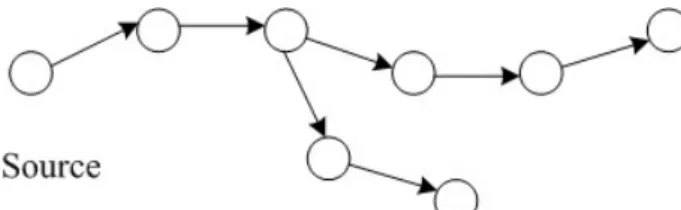
(12) example, if application layer multicast using tree structure, one peer needs to retransmit the streaming data to several peers in the same time. But upstream bandwidth might be very less than downstream bandwidth. The lack of upstream bandwidth will cause the performance of application layer multicast being poor. Otherwise, the application layer multicast can only provide low quality data streaming service. In the present day, the data rate of most data streaming service on the Internet is around 300 to 500 Kbps [24], [25]. If we have no abundant bandwidth and want to provide streaming data to others, all we can do is use application layer multicast. When some receivers are the peers with asymmetric connectivity, it will bring an issue that they can only retransmit data to very few peers. (In Taiwan, the maximum upstream bandwidth of asymmetric connectivity is 1 Mbps and the general is 512 Kbps [20].) This issue will limit the amount of peers that can join the service or the quality of streaming data the service can provide will be poor. Furthermore, because the degree of nodes in the tree is few, the height of the tee will be bigger and the end to end delay from source to peers will be larger. There is an example in Figure 1. Furthermore, in some special cases, if the number of users that want to join the service is few, we can’t even build a workable tree between them because the choice of parent is few.. Figure 1: Large end to end delay when node degree is few. 1.2 Research Approach The name of the scheme we propose is called Trickle. The transmission paths among peers will be tree structure. In current stage, we don’t focus on how to build a tree among peers. Our purpose is to improve resilience of existent tree building algorithm by integrated 2.

(13) with Trickle. Moreover, Trickle won’t violate decentralized control if the tree building algorithm is decentralized. Following, we will define the meaning of resilience and then introduce our three approaches: information dispersal algorithm, multiple stripes, and helper.. 1.2.1 Definition of Resilience We will devise a resilient application layer multicast approach including fault tolerance, robustness, security, and solving asymmetric connectivity issue. For fault tolerance, peers can tolerate a small number of packet delay or loss and they still can receive complete message in time. For robustness, a sudden breakdown of some peers or links won’t disrupt reception of downstream peers. For security, we provide a partial security protection for streaming data.. 1.2.2 Three Approaches Information dispersal algorithm (IDA) [8] IDA will be used to process the message generated from source peer and divide the message into several pieces. Peers can restore message from a part of message pieces. We use IDA for two purposes: (1) peers don’t need to receive whole pieces of a message and they still can have the complete message. It will improve the resilience of data transmission, (2) peers can’t know any content of the message if they don’t have enough pieces. Therefore, if some peers have no authority to read the message, we only need to make sure not to let them receive too many pieces of the message. In short, the participation of helper is the main reason we want to enhance security. Multiple stripes The pieces of messages divided by IDA approach is called stripes. In tree building step, we not only construct one tree, we construct as many different trees as the number of stripes that one message is divided into. And each tree transmits different stripe of the message. This approach will lead to two advantages. First, it can make sure that peers can receive enough stripes. When one peer leaves or crashed, descendants of the peer will only lose one stripes and they still can receive other stripes from other trees. Furthermore, when a link of tree is congested, it only makes one stripe delay. Second, every peer can fully utilize. 3.

(14) their upstream bandwidth. A stripe is much smaller than a message, so peers with low upstream bandwidth can also support several children. Helper Because the lack of upstream bandwidth, it is possible that new peers can not find a parent in the tree that can provide them smooth streaming data. It is because the peers in the trees can support no more children or because the peers can support more children is far from new peers. Therefore, the service will request some peers called helpers that still have unnecessary bandwidth to join and share their bandwidth to increase the total mount of upstream bandwidth of the service. By the help of helper, the service can accept more peers and each peer can receive the streaming data smoothly by having better parent choices.. 1.3 Outline of Thesis In chapter 2, we will briefly introduce three different architecture of multicast and the related work of application layer multicast. In chapter 3, we will describe the detail of the three approaches. In chapter 4, we will describe the use of three approaches in the mechanism of application layer multicast and how it works. In chapter 5, we will show the simulation results and evaluate our performance. In chapter 6, it is the conclusion and the future work.. 4.

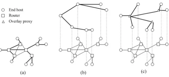
(15) Chapter 2 Background 2.1 Architecture of Multicast Since multi-receiver multimedia applications, like video-conferencing, video streaming, e-learning and online-gaming, are more and more popular on the Internet, multicast is an important mechanism need to be developed. Multicast is a one-to-many transmission mechanism and is very efficient to reduce duplicate packets and bandwidth consumption when it is used for multi-receiver applications. There are three different architecture of multicast: IP multicast, application layer multicast (ALM), and overlay multicast [21]. Figure 2 shows the difference between these three architecture clearly. IP multicast is developed on network layer and use routers as the relaying nodes. IP multicast is the most directly implementation of multicast and can reduce most duplicate packets in transmission process. However, because of several issues [1], IP multicast is not globally deployed yet.. Figure 2: Three different architecture of multicast. (a) IP multicast, (b) application layer multicast, (c) overlay multicast. 5.

(16) Overlay multicast is the architecture that constructs a backbone by overlay proxy first. And then it establishes multicast trees among overlay proxy and end hosts. It has good performance that is close to IP multicast. However, the main issue is the deployment of overlay proxy. Application layer multicast is a hot research topic in recent few years [2~5, 7, 11, 12, 14, 16] and has become an attractive solution of multicast. It is also the easiest one for immediate deployment among these three architectures. ALM is developed on application layer and doesn’t need to modify any existent protocol in lower layer. User’s desktops or mobile devices (called peer) replace the function of routers in IP multicast. Data packets are replicated at peers and send to other peers in the same application layer multicast service.. 2.2 Related Work We briefly introduce some research about application layer multicast.. 2.2.1 Multiple Description Coding (MDC) The overview of multiple description coding is in [22]. It is a method to encode signal into multiple separate descriptions (streams) and any subset of descriptions can be restore to the original signal with different quality. If users receive more description, the distortion will be less and the quality of restored signal will be higher. One difference between MDC and IDA is MDC is a source coding method and IDA is a channel coding method.. 2.2.2 Multiple Stripes SplitStream [2] and CoopNet [3] are two mechanisms using multiple stripes. Both of them get a result that using multiple stripes will increase the robustness, resilience, and load balance. The detail of multiple stripes will be described in next chapter. There are two main differences between them. First, CoopNet uses a centralized tree building algorithm while SplitStream is decentralized because it bases on Scribe. Second, CoopNet does not handle the. 6.

(17) bandwidth contribution of peers in the trees.. 2.2.3 Waypoint There is new overlay architecture in [9]. Besides normal participants, they employ some machines call waypoints. In the overlay tree, these two kinds of nodes are interwoven. It is different to the overlay proxy in overlay multicast. Waypoints are the same as normal participants and they run the same protocol. Therefore, its behavior is the same as other users, rather than statically provisioned infrastructure nodes, such as Overcast nodes in [6]. The purpose of waypoint’s participation is to increase the total amount of resource in the system. In their experiences, waypoint is needed in some cases and their investigation is still in progress. Besides, the difference between waypoint and helper will be described in next chapter.. 2.2.4 Tree Building Algorithm The two main categories of tree building are based on distributed hash table (DHT) and hierarchical clustering. Scribe [14] and Bayeux [16] are the ALM tree building methods that base on the Pastry [13] and Tapestry [15] DHT mechanism. In the beginning, the purpose of DHT is to search and route efficiently (with the bound of hops, usually log(N) hops). Every peer will be assigned an id that generated by hash mechanism and the routing path will base on the hash id. And then, the tree building methods that base on DHT build transmission paths along the routing path by reverse path forwarding (RPF) method. These transmission paths have same source peer, so these paths will form a tree structure. NICE [4] and ZIGZAG [5] are the ALM tree building methods that base on hierarchical clustering. Each peer who wants to join the tree will be put into a cluster base on specified metrics (such as distance). One or more peers in the cluster will be promoted to a higher level cluster and their responsibility is to transmit data to all peers in lower level cluster. And then, there is also a higher level cluster to send data to the high level clusters. Finally, the only one member in the highest level cluster will be the source peer. These clusters construct a tree 7.

(18) structure and a level of clusters represents a level of the tree.. 2.2.5 Enhancement of Resilience Probabilistic Resilient Multicast (PRM) [11] uses a proactive forwarding approach to increase the data delivery ratio. The method is to use randomized forwarding. Every node randomly chooses a constant number of other nodes and forwards data to them with low probability. The randomized forwarding is simultaneous with the usual data forwarding mechanism. Hence, some nodes may receive the same data. But this approach will make the nodes can receive the data even when their parents fail. And then, it proposes an extension called Ephemeral Guaranteed Forwarding (EGF). When some nodes are repairing their transmission paths (finding new parents), they can request other nodes to temporarily increase the probability of forwarding data to them. Therefore, they still can receive the data in the repairing process. A proactive approach to reconstruct multicast trees is proposed in [12]. When some interior nodes leave trees or fail, it will minimize the disruption of service for those affected nodes. The approach is every interior node should compute a parent-to-be for each of its children. In the computation process, it will consider the degree constraints of each node. And it also deals with the situation of multiple leaves. After that, if an interior node leaves the tree or fails, all its children will find their new parent (parent-to-be) immediately. By this approach, when some edges of the tree broken, every node can find a new parent quickly and also recover the transmission path.. 8.

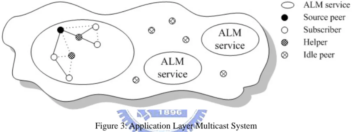
(19) Chapter 3 Principle 3.1 Overall System The three approaches we use are information dispersal algorithm, multiple stripes, and helper. Base on these three approaches, we can establish the scheme of application layer multicast system presented in Figure 3.. Figure 3: Application Layer Multicast System. The whole graph is an ALM system with many independent ALM services inside. Each service provides different streaming data. The circle nodes are the users who join the system and generally called peer. Each peer has different name based on what they do in the system. Peers who provide streaming data are called source peers. Peers who subscribe the service are called subscribers. Peers who don’t subscribe the service are called helpers of the service. Peers who don’t subscribe any service are called idle peers and they can be helpers for all services. Now, we point out the place our three approaches performed. Information dispersal algorithm The dark circle node is the source peer. Before it sends out the streaming data, the data will be processed by IDA. Multiple stripes In Figure 3, there are two different lines inside the ALM service in left side. The two kinds of line represent two different trees and source peer transmit different 9.

(20) stripes which are generated from IDA through different trees. Helper The ALM service in left side shows there are two helpers contribute their bandwidth to the service. They help to retransmit stripes to the subscribers of the service. We have several hypotheses for the ALM system. One, most peers of the ALM system are using asymmetric connectivity. It means they have poor upstream bandwidth. Two, all peers have degree constraint which is determined by the upstream bandwidth offered by individual peers. Three, the data rate of the streaming data provided in ALM system is too high for general ALM mechanism. Four, the number of peers in the ALM system is very large. In other words, the lack of helper is not a problem. Five, the streaming data transmitted in ALM service might have security requirement. In the following sections, we will introduce the principle detail of the three approaches.. 3.2 Information Dispersal Algorithm (IDA) (n, m) information dispersal algorithm (IDA) [8] is a method that disperses data for security, fault tolerance and etc. It can disperse the original data into n pieces and we must have m pieces or more, m ≤ n , to be able to restore to the original data. For security, peers can’t know any content of data if they have less than m pieces. For fault tolerance, it means that it could tolerate some of pieces missing and still can restore to the original data. Moreover, it has a special characteristic that the m pieces we mention before is any m pieces without any order, needn’t to be continues, and no any piece is must have. On the contrary, using IDA will cause the data size much bigger. If the size of data F is F , we disperse it into n pieces, the size of each piece will be F / m . Therefore, the total size of n pieces will be F ⋅ ( n / m ) . Following we will brief describe how to use IDA in transmission process.. 3.2.1 Split First, we must decide (n, m) and then we use IDA on the transmitted data F. Let the 10.

(21) content of F be b1 , b2 ,… , bN , F is divided into N units. We use the content of F to generate a matrix B and the blank places are filled in 0. The size of matrix B is m × ⎢⎡ N / m ⎥⎤ .. F = b1 , b2 ,… , bN = (b1 , b2 ,… , bm ),(bm +1 , bm +2 ,… , b2 m ),… ⎛ b1 ⎜ b B=⎜ 2 ⎜ ⎜⎜ ⎝ bm. bm+1 bm+2 b2 m. b⎡⎢ N / m⎤⎥ ⎞ ⎟ ⎟ ⎟ bN ⎟ 0 ⎟⎠. (1). (2). Then we choose n vectors ai , 1 ≤ i ≤ n , and the length of each vector is m. Every subset of m different vectors must be linearly independent. And then we use ai to compose matrix A that the size of matrix A is n × m .. ai = ( ai1 ,… , aim ), 1 ≤ i ≤ n. (3). ⎛ a1 ⎞ ⎜a ⎟ A=⎜ 2⎟ ⎜ ⎟ ⎜ ⎟ ⎝ an ⎠. (4). It is the initialization step from (1) to (4). Then we will use IDA in the transmission process. First, we will divide F into n pieces. Base on the matrix A and B we calculate before, A ⋅ B = C , C is a n × ⎡⎢ N / m ⎤⎥ matrix. We can divide C into n vectors called ci , 1 ≤ i ≤ n ,. the length of a vector is ⎡⎢ N / m ⎤⎥ . These n vectors are the pieces we want. And then these n pieces will be transmitted through different transmission paths to all peers (based on multiple stripes approach).. ⎛ c1 ⎞ ⎜c ⎟ A⋅ B = ⎜ 2 ⎟ = C ⎜ ⎟ ⎜ ⎟ ⎝ cn ⎠. (5). ci = ( ci1 , ci 2 ,… , c⎢⎡ N / m ⎥⎤ ). (6). 11.

(22) cik = ai1 ⋅ b( k −1) m+1 +. + aim ⋅ bkm. (7). 3.2.2 Restoration After splitting F into n pieces in previous section, we will show we can restore F from any m pieces. When peer receives m pieces or more, the peer can restore the original F. We choose any m pieces. ( ci ,ci +1 ,… , ci +m ) and choose the corresponding m vectors. (ai , ai +1 ,…, ai + m ) in A. Through the expression below, we can restore the matrix B and also we obtain the original data F. −1. ⎛ ai ⎞ ⎛ ci ⎞ ⎜a ⎟ ⎜c ⎟ B = ⎜ i +1 ⎟ ⋅ ⎜ i +1 ⎟ ⎜ ⎟ ⎜ ⎟ ⎜ ⎟ ⎜ ⎟ ⎝ ai +m ⎠ ⎝ ci +m ⎠. (8). Therefore, as long as all peers generate the same matrix A as source peer, they could restore the original data from any m pieces of the data.. 3.2.3 Efficiency Only produce matrix C and restore matrix B in IDA will influence on the efficiency of Trickle. It is because the production of matrix A and A-1 is only once, we don’t need to reproduce. Now, we consider the number of operations split and restoration need. For split, it needs n × m × ⎡⎢ N / m ⎤⎥ multiplication operations and n × ( m − 1) × ⎡⎢ N / m ⎤⎥ addition operations. The complexity of operation is also associated with the size of b which is F / N . Therefore, split is affected by the parameter n and the size of data. The complexity of. split is O ( n × F ) . For restoration, it needs m × m × ⎡⎢ N / m ⎤⎥ multiplication operations and m × ( m − 1) × ⎡⎢ N / m ⎤⎥ addition operations. Therefore, restoration is affected by the parameter. m and the size of data. The complexity of restoration is O ( m × F ) .. 12.

(23) 3.2.4 Advantage Using the combination of IDA and multiple stripes in transmission process has several advantages. First, security and fault tolerance, these are the design purposes of IDA. These two characteristics quite match our requirement. Because we join the concept of helper into Trickle, security of data transmission is necessary when the data is sensitive. And further, because the whole ALM service is composed by peers (end hosts), the service can’t promise peers can receive all data. By the fault tolerance of IDA, the transmission process is more resilient. Second, we only need to receive m of n pieces to restore original data, so we do not need to wait the remand n-m pieces. Because every piece is transmitted through different path, some paths are congested and some are not. Therefore, the thing that influences on our delay of receiving data is the most quick m paths, not all n paths. Even if the congestion of transmission paths will change, we still can prevent to be influenced by most congested n-m paths without changing our transmission paths. Hence, the receiving process is more efficient.. 3.2.5 Influence of n and m Because our IDA and multiple stripes approach will influence each other, the decision of n and m will cause some effect. First, n will influence on how many trees we will build in an ALM service. Too many trees will lead to increase amount of control signal and the control overhead will consume our rare upstream bandwidth. Second, the ratio of n and m will influence on the transmission overhead. As we mention before, the size of data that using IDA will ( n / m) times bigger than the original one. It means that the data transmitted through network will increase ( n / m) times. However, we don’t really need to receive all n stripes. We will explain the improvement in next chapter. In addition, the ratio of n and m will influence on the resilience of ALM service. The larger ratio of n and m is, the more resilient ALM service will be. In other words, we can tolerate more stripes lose. Hence, the decision of n and m is very important and must base on what application the service wants to provide.. 13.

(24) 3.3 Multiple Stripes/Trees The concept of multiple stripes has been brought up in previous research [2], [3]. Each message transported from source peer will be divided into several stripes. In tree building step, we not only construct one tree, we construct as many different trees as the number of stripes that one message is divided into. And each tree transmits different stripe of the message to subscribers. Hence, the peer receives different stripes of the message through different transmission paths. Figure 4 present an example of multiple stripes. By this approach, we get a lot of advantages mentioned before. Moreover, we enhance multiple stripes by combining with IDA approach. The description is in following content.. Figure 4: An example that a message is divided into 2 stripes. 3.3.1 Combine with IDA The combination of multiple stripes and IDA mean that one message will be divided into several stripes by IDA approach. And each stripe will be transmitted through different trees. The purpose of multiple stripes/trees is to prevent losing a whole message when one link broken. The purpose of IDA is to promise peers will restore the original message even some stripes lose. When we use (n, m) IDA technology, every peer joining in the ALM service will have n different transmission paths (actually, it is mostly less than n, we will explain about it in next chapter) that the origination is source peer and destination is itself. Each transmission path of the peer transmits different stripe and peers only need to receive any m stripes of the total n. 14.

(25) stripes, then those stripes can be restored to the original message. In other words, the transmission process can tolerate to loss at most n-m stripes. Therefore, we must make sure that any peer leave the ALM service will not cause the remand peers who are still in the ALM service can not restore the original message. This situation happens only when the leaving peer is in more than n-m of n transmission paths of any peer. When such peer leaves the ALM service, it will cause more than n-m transmission paths of the peer break down and the peer can only receive less than m stripes. Hence, the peer can not restore the original message. This situation can be prevented by building disjoint transmission paths.. 3.3.2 Building Disjoint Paths Base on the description before, we know that we must prevent any peer is in more than n-m transmission path of other peers. The solution for building this kind of transmission paths is to restrict that every peer become interior node in constant number of trees. And the number must not bigger than n-m. Therefore, there are two different choices to decide the number of being interior node for each peer. The first choice is every peer becomes interior node in more than one tree and the second choice is to restrict every peer can become interior node in only one tree. The advantage of first choice is that some peers with high upstream bandwidth will contribute their bandwidth averagely in multiple trees without contributing whole upstream bandwidth in only one tree. It is good for Trickle because in transmission process with IDA, the importance of all stripes is the same. However, there is a critical disadvantage to contribute bandwidth in multiple trees. It will cause the height of trees in ALM service much bigger and the end to end delay will be higher because the degree of nodes in each tree are smaller. Therefore we decide to pick the second choice that every peer becomes interior node in only one tree. This method restrict that any peer at most in one of n transmission paths of other subscribers. And then, we have to use a method to decide peers become interior node in 15.

(26) which tree. In SplitStream [2], it provides a method that can establish interior-node-disjoint trees. Each tree root has different prefix of groupId. Due to the tree building method, groupId and nodeId of peers will cause which peers become interior node. Therefore, it will restrict that every peer will play the role of interior node in no more than one tree and being leaf node in the remand trees. This method is only fit for the tree building algorithms that base on DHT. In out hypothesis, we hope Trickle can be applied to any tree building algorithm. Therefore, we use different method to decide peers become interior node in which tree.. 3.3.3 Become Interior Node Each peer decides it will become interior node in which tree by itself. When a new peer is in the process of joining service, there are two decision methods to decide which tree it should be interior node. One, in order to prevent violating the DHT concept, if the tree building algorithm is based on DHT, it decides to be interior node in the tree whose root has the same prefix hash id. It is approximately the same as SplitStream, but the only difference is the peer already decides the tree it wants to be interior node by itself in the beginning of joining service. The second method is the peer randomly decides which tree it should be interior node and be leaf node in other trees. The advantage of random solution is that we don’t need a server to do resource (upstream bandwidth) management. However, it may probably cause large number of peer being interior node in the same tree and the resource distributed unfairness. It will cause that the upstream bandwidth of some trees is not enough. We solve this problem by using the concept of helper. Those trees with poor resource will ask helper for help. The helper will share their upstream bandwidth to those trees that need it. Therefore, when the number of helper is nearly infinite, the upstream bandwidth won’t be exhausted. And the concept of helper will be described in next section.. 16.

(27) 3.4 Helper The peers are idle or the subscribers of other services can be the helper of the service. For example, in one service, the peers are regarded as subscribers, but for other services in ALM system, they are not subscribers. Therefore, we call them helper when they are not regarded as subscribers of the service. We hope those peers that are idle or have ample upstream bandwidth can share their bandwidth with other ALM services. Hence, for those ALM services that can not provide smooth streaming data to the subscribers will request helper for help.. 3.4.1 Demand of Helper In order to make every peer receive streaming data smoothly, every peer will restrict the number of children it can support based on its upstream bandwidth. A peer will request to be some peer’s child in three cases: (1) the peer is a new subscriber and it chooses a peer in the service to be its parent by tree building algorithm, (2) the transmission path between the peer and source is broken, it wants to change transmission path, (3) the tree structure adaptation algorithm will cause peers to change their parents. When the peer already reaches its upper bound of child number, it receives the request from the other peer that wants to be its child. It is the time to request helper’s help in order to accept the request.. 3.4.2 Find Helper There are two issues need to be consider when peers need helper’s help. How to find the helper Because we expect our infrastructure of ALM system is based on decentralized control, not centralized control by some peers, like source peer. Hence, every peer needs to have the capability of finding helper. When every peer joins the ALM system, they will establish a neighbor table to record peers that are close to them. The definition of neighbor is that the number of IP routing hops between its neighbor and itself is below a predefined number. When the peer joins one ALM service and the neighbors of the peer who. 17.

(28) are not in this service can be helper candidates (because of the restriction in next section). Hence, peers can request assistance of helper candidates in neighbor table when they need helper’s help. Helper selection The second issue is that if there is more than one helper candidate, which one of candidates we should choose. Because the participation of helper will make the transmission path longer and it will increase the end to end delay of affected peers, we must choose the candidate that increases the transmission path length least. We explain it by an example presented in Figure 5. dAH means the number of IP routing hops from A to helper candidate (who are in the neighbor table of A), dHB means the number of IP routing hops from helper candidate to B. If we need the assistance of helper between A and B, we will choose the candidate that it makes the dAH+dHB to be smallest and then we request the helper candidate to join the ALM service and place it between A and B.. Figure 5: An illustration of helper selection. 3.4.3 Restriction of Helper The selection of helper has two restrictions. First, helper might be the subscriber of other ALM service. We can not request them to share too much bandwidth that will cause them can not smoothly receive the streaming data they want. Therefore, every peer will share the fix ratio of bandwidth for being helper. The ratio of bandwidth it will share is defined by ALM system. Second, for security consideration, we can’t allow helper to know the content they transmit. Base on the characteristic of (n, m) IDA, we restrict a helper can help only one tree in one ALM service. It means a helper can only join one tree of the service and become interior node in the tree. Hence, helper can’t know the content it transmits because it doesn’t have enough stripes. And also, every peer still can receive the whole message when it leaves. 18.

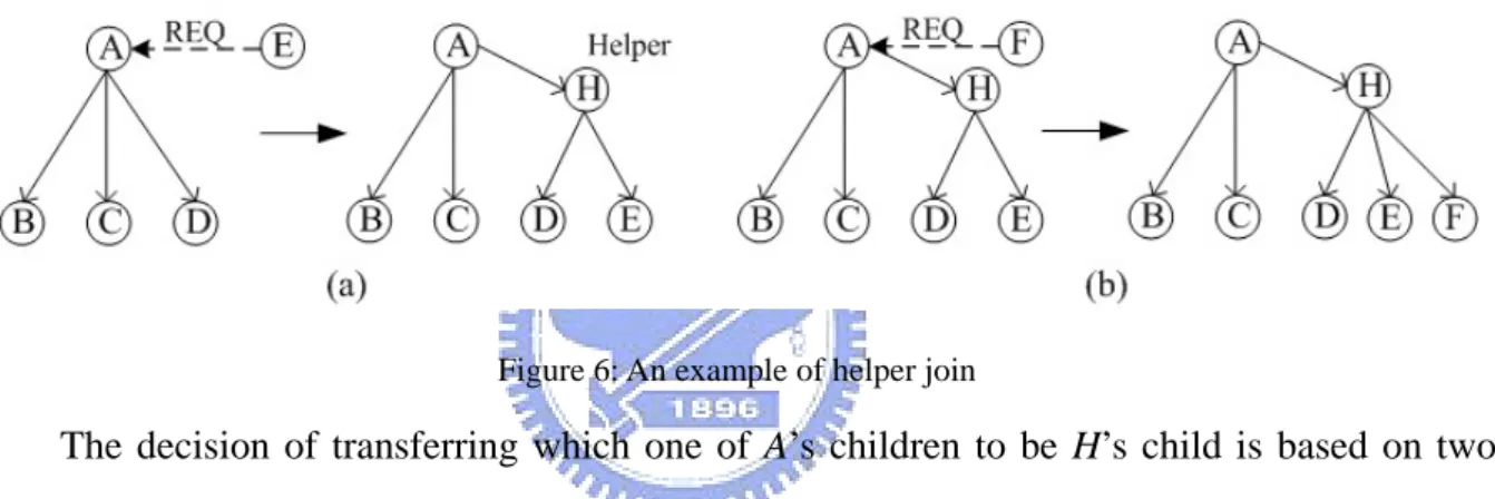
(29) 3.4.4 Helper Join After finding one helper, we need to explain how the helper joins the tree. We explain the process by an example presented in Figure 6. In Figure 6(a), peer A’s upper bound of child number is 3. It shows A is already reach its upper bound and new peer E send request to A that it wants to be A’s child. It is the situation that needs helper’s help. There are three steps to make a help joining the tree. First step, peer A chooses helper H from helper candidates by the method described in previous section. Second step, peer H becomes A’s child and accepts E’s request, so E becomes H’s child. Third step, peer A transfers its child D to H and D becomes H’s child.. Figure 6: An example of helper join. The decision of transferring which one of A’s children to be H’s child is based on two rules. Rule one is leaf node has higher priority and rule two is choose the one closest to helper. If some of A’s children are leaf nodes, we choose the leaf node that is closest to H. Otherwise, we choose the one of A’s children that is closet to H. We choose leaf node first because it won’t affect too much peers who will increase end to end delay. In this approach, the ALM service can successfully accept peer E. It will bring two advantages. First, E request to be A’s child who is already reach its supporting upper bound must because it is E’s best choice or the only choice. Because we expect our infrastructure is decentralized control; usually, E can only obtain a small part of peers’ information in the ALM service. Therefore, the parent choice of E is limited. Hence, base on this approach we could successfully accept E and also try our best to prevent to influence on peers that are already in the service. Second, because H is A’s neighbor, when H joins the service, the peers who might 19.

(30) choose A before could have another choice H. Therefore, peers can have more choices. Moreover, H still not reaches its upper bound of child number. It increases the number of peers the tree can support.. 3.4.5 Enhancement Enhancement 1 In finding helper step, we don’t really need to choose the neighbors that are not in the service to be helper candidates in an exception. When the neighbor is already in the service, if the tree needs help is the same tree it already in, we still can request its help. In Figure 6(b), a new request from F, if the best choice of helper is still H, then A still can request H’s help if H doesn’t reach its upper bound of child number. In addition, in this case, child transfer step can be omitted. Enhancement 2 By enhancement 1, the peer may find a helper that is other peer’s child. In this case, the helper can change parent if the distance from source peer to it will be shorter. We explain it by an example presented in Figure 7. dSA is the distance between source peer and peer A, dSB is the distance between source peer and peer B, dAH is the distance between peer A and peer H, and dBH is the distance between peer B and peer H. When peer B receives a request from Z, B detects the best helper is H and requests H’s help. There are two possible results. If (dSA+dAH) ≤ (dSB+dBH), the result is presented in Figure 7(b). If (dSA+dAH)>(dSB+dBH), the result is presented in Figure 7(c). By this enhancement, not only helper will have lower end to end delay, but also all its children and descendants.. Figure 7: An example of helper approach enhancement. 20.

(31) 3.4.6 Difference between Helper and Waypoint There is already a similar concept to helper called waypoint [9]. Both helper and waypoint are the peers with unnecessary resource, such as upstream bandwidth, and they provide it to help others. The most different point between waypoint and helper is that waypoint joins the service base on its own decision and helper joins the service when members in the service call for help. The concept of waypoint is to treat waypoint as common peers. It means that the method of joining service and the data it receive is the same as common peers. Even though waypoint will join the service that need help base on its determination, its join method is the same as other peers. It may not be put in the urgent place that needs help. For example, there is one sub-tree in the service needs help. Waypoint may join this service, but may not be put in that sub-tree by the join mechanism. Contrary, helper is requested by the members in the service who need help. And the helper joins the service using different joining mechanism. Helper will be put in the place that really needs help. Therefore, participation of helper will solve the issue immediately.. 21.

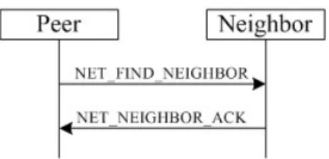
(32) Chapter 4 Mechanism In this chapter, we will introduce the mechanism of ALM service and the integration of our three approaches in the mechanism. We separate the mechanism into two parts. The first part is the start of an ALM service and the second part is the behavior of peers.. 4.1 Service Startup There are three things need to be done to start an ALM service in the ALM system. First, every peer should establish a neighbor table before join or start a service. Second, if a peer wants to establish an ALM service to share its streaming data, it must decide who the source peer of the service is. Third, the source peer must configure IDA before accepting subscribers. We describe the details in the following content.. 4.1.1 Establish Neighbor Table Before ALM service start, every peer who wants to join the ALM system, including source peers, subscribers, and even helpers, should establish their own neighbor table. The establishment of neighbor table is prerequisite for our helper approach. The negotiation between peers and their neighbors is presented in Figure 8. We define a neighbor finding signal. In that signal, we set within how many hop count the peer can be called neighbor and the signal is sent by broadcast method. The signal should be drop when it travels farther than neighbor distance. When peers receive a neighbor finding signal, they should reply an ack signal to original sender.. 22.

(33) Figure 8: Negotiation between peers and neighbors. If a peer receives an ack signal from other peer, it means it find a neighbor. The peer should do the reaction presented in Table 1. If the neighbor table is not full, it just adds the sender of the ack signal into the table. If the neighbor table is full, when the sender is closer to it, it just adds it into table and removes the neighbor that is farthest to it. After repeatedly receive the ack signals and do the reaction described above, peer will obtain a neighbor table with closest neighbors inside. Be notice that the neighbor table should resize if there is no any available neighbor when peers need neighbor in Trickle.. Table 1: Reaction after receiving a neighbor ack message. 4.1.2 Source of Service Source peer is the tree roots of the service. It splits streaming data into IDA stripes and sends stripes to its children of each tree. But which peer is the source peer? Is the streaming data owner should be the source peer of the service? It is possible, but not necessary. There are two possible cases. Source peer is the data owner When the data owner is a peer with sufficient upstream bandwidth and processing capability, such as multimedia service provider, it could be the source peer of the service. Source peer is not the data owner When the data owner is an individual user, it. 23.

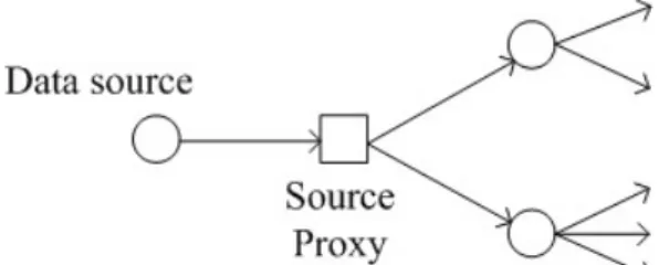
(34) probably only can unicast the data to one child. All it can do is to send the streaming data to a proxy server (we call source proxy) with capability of being source peer and the IDA is done by source proxy. It is presented in Figure 9. The source proxy can be the e-home server. Users send data from their mobile devices to their e-home server and then the server multicasts data to numerous peers. Or the source proxy can be provided by ISP with commercial cost. There still has a lot of possibility about the source proxy. It can solve the issue that data owner is not powerful.. Figure 9: An illustration that source peer is a source proxy. 4.1.3 IDA Configuration 4.1.3.1 (n, o, m) IDA After deciding which peer is the source peer, source peer must decide the parameters of IDA. In the previous chapter, we mention we will combine multiple stripes and IDA. However, we don’t adopt (n, m) IDA but (n, o, m) IDA. All we want to do is to decrease bandwidth consumption from the overhead of IDA. First, n means in the ALM service, there will be n different trees. The message generated from source peer will be divided into n different stripes and each stripe will be transmitted in different tree. Second, m means every peer that join the service must receive at least m stripes of a message to restore to the original message. Third, o means that when every subscriber wants to join the ALM service, they should join o trees initially, n ≥ o > m . We have to explain about the range of o, n ≥ o > m . The IDA operation is decided when the ALM service starting, so n and m can’t be changed. Hence, there will be totally n trees, so o must less or equal n. And o must bigger than m is because we don’t want when any peer leave the service will cause any other peers that is still in the service can not receive m stripes of the message. 24.

(35) Due to we restrict every peer can be interior node in only one tree, so the lower bound of o is m+1. And if we want to decrease the consumption of the bandwidth, we must set o closer to m. Because o > m , it still can provide a little fault tolerance in normal situation. 4.1.3.2 Apply to Streaming Data Now, the source peer can apply IDA to streaming data when subscribers join the service. The (n, o, m) parameters will influence on two things: the size overhead and the fault tolerance of the service. If the size of unit message needs to be encoded by IDA is B and we apply (n, o, m) IDA to it, the size of one stripe will be B/m and the total size of stripes is n × B / m . Each subscriber need receive o stripes with size o × B / m in the beginning. The. ratio of lost stripes subscribers can tolerate is between (o − m) / o to (n − m) / n . 4.1.3.3 Discussion The reason we add the parameter o is because when a message is processed by IDA, the size of the message will be (n/m) times bigger. If every subscriber joins n trees in the beginning, it will consume too much downstream bandwidth of itself. ((n-m)/m of data is redundant.) In other words, it will consume too much upstream bandwidth of other peers. In order to prevent it happens, we must make every peer to receive redundant stripes as less as possible. First, we must consider why peers need to receive redundant stripes. The peer receive more than m stripes of a message is because we promise when some stripes delay or lost, they still can restore to the original message without any delay (there are the upper bound of tolerance). Therefore, we need to receive more stripes (join more trees) of one message only when some stripes’ transmission process occur problems. But we still need to receive a little part of redundant stripes (o-m stripes) in normal situation. Otherwise, we will lose one or more message when we are doing remedial action. Oppositely, if the transmission process of stripes has no problem, we should receive stripes as less as possible (join less trees) to prevent the consumption of bandwidth. Hence, after the peer joins o trees in the beginning, every peer 25.

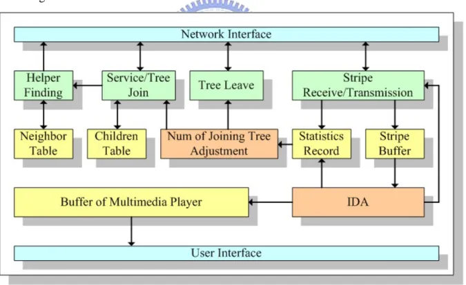
(36) should adjust the number of trees they join dynamically. The method about how to decide the adjustment will be described in later section.. 4.2 Behavior of Peers First, we describe the architecture of peer behaviors. And then we describe the detail of each behavior. The order of behaviors is organized along peer life cycle.. 4.2.1 Architecture of Peer Behavior The architecture of behaviors for peers that will be subscribers or helpers is presented in Figure 10. Arrow symbols mean the direction of data flow or control signals. It shows the interaction of each function and the detail of important behaviors will be described in following sections.. Figure 10: Architecture of peer behavior. 4.2.2 Join 4.2.2.1 Randomly Join o Trees When the peer decides to join an ALM service, it will know the n, o, and m parameters of the service. Hence, the peer knows it must join o trees of the service initially. In Trickle, the 26.

(37) method that peers decide they should join which trees is random selection by themselves. The reason is the same as randomly select a tree to be interior node. We don’t want to add a load balance manager or request any peer, such as source peer, to be responsible for it. Management of network load will increase the load of peer and also waste bandwidth. Let us consider the tradeoff of load balance. First, it will make every peer fairly consumes upstream bandwidth. It is not an advantage for our hypothesis. For our helper approach, because the lack of upstream bandwidth, if some peers don’t spend all their upstream bandwidth in the service, they will possibly spend remained upstream bandwidth in other services. Therefore, there is no benefit in this point. Second, load balance will lead the peers distributed averagely. In other words, the height of each tree in the service will be average. It is really an advantage because the end to end delay of all peers will be average. However, in Trickle, we have done several steps to reach similar effect. One, we make every peer join o trees. In worst case that all subscribers join the same o trees, the load is still averagely distributed into o trees. Two, because of IDA, peers can ignore some worse stripes with high end to end delay in certain trees. Three, the trees and the number of trees each peer joins will change to have better performance. It will be mentioned in following section. Of course, load balance is the best choice, but by these three steps, the end to end delay of the peers will be lease and more average. Furthermore, we don’t need to waste bandwidth to maintain load balance. Therefore, we decide that every peer randomly chooses o trees to join. And then they randomly choose one of o trees to be interior node. 4.2.2.2 Choose Parents After each peer chooses which o trees they want to join, they must decide which peer should be their parent in each tree. The selection method of parent is based on tree building algorithm. Our purpose is to devise an approach that is able to suit any tree building algorithm for performance improvement. So any kind of tree building method, like distributed hash tables (DHT) [14], [16] or hierarchical clustering [4], [5], will be fine. The method only needs 27.

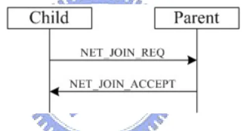
(38) to build one tree and other tree can also be built by the same method. Therefore, each new peer will find o parents in different o trees through tree building algorithm. No matter what tree building algorithm the ALM system choose, we have to add two restrictions for the algorithm. The first restriction is it can’t choose peer that plays the role of leaf node to be any peer’s parent. The second restriction is every peer should have an upper bound of supporting children base on their upstream bandwidth for performance consideration. 4.2.2.3 Cases of Join Accept There are two cases when peers receive a join request. The first case is presented in Figure 11. If the peer plays the role of interior node in the tree and still has quota to accept new child, then it accept the request and put the id of request sender into its children table.. Figure 11: Negotiation between child and parent. The second case is presented in Figure 12. If the peer that receives a join request already reaches its upper bound of child number, it will request a helper for help. And it also needs to transfer one of its children to be the helper’s child. The detail of using helper is already described in previous chapter. Sometimes, request helper’s help will fail when helper receives the request and it already reaches its upper bound of child number or it already joins other tree. Figure 13 presents the failure of requesting helper.. 28.

(39) Figure 12: Negotiation between child, parent, and helper. Figure 13: Negotiation after the failure of requesting helper. We combine the two cases into one flowchart and it is presented in Figure 14. And the detail reaction when parent receive the join request from a peer is presented in Table 2.. Figure 14: Flowchart of subscriber join. 29.

(40) Table 2: Reaction after receiving join request. 4.2.3 Receive and Retransmit For source peer, transmission process is simple. Its responsibility is to generate n stripes using IDA from original data and transmit each different stripe to its corresponding children set in different trees. It is presented in Figure 15. And for peers that are leaf nodes in the tree, all they have to do is wait and receive stripes transmitted from parents. But for other peers that are interior nodes in the tree, there are two different ways to do the retransmission.. Figure 15: An illustration of stripe transmission for source peer. 4.2.3.1 General Retransmission When the peers play the role of interior node in the tree, they have responsibility to retransmit the corresponding stripe to their children. For example, if the peer is interior node in tree k, it must transmit stripe k of the message to its children in tree k. In general case of retransmission, when peers receive a stripe from parent in the tree that they serve as interior node, they just retransmit the stripe to their children. It is presented in Figure 16. So they have. 30.

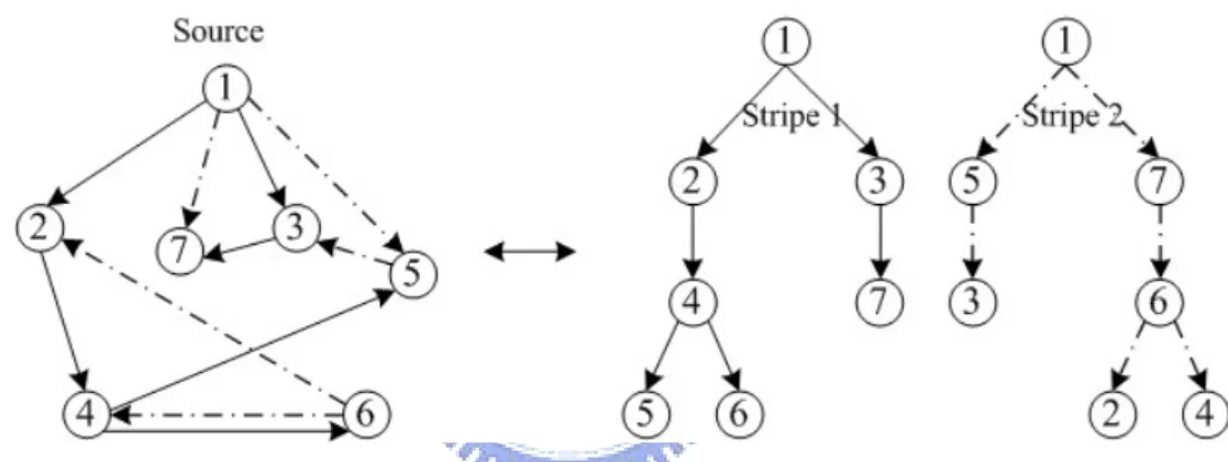
(41) done their responsibility. This is the basic concept of any ALM mechanism.. Figure 16: Peers retransmission. 4.2.3.2 Stripe Regeneration Because we use multiple stripes and IDA approaches, peers can regenerate any stripe they need to retransmit (even if they never receive it) and transmit to their child. The algorithm of stripe regeneration is presented in Table 3. When the peer already receives m stripes of the message from other trees but not including the stripe it need to retransmit, it can use these m stripes and matrix A of IDA to restore them to the original message. And then base on the original message and matrix A, it can generate any one of n stripes it needs.. Table 3: Reaction after receiving one stripe. For example, in Figure 17, peer A join 5 trees to receive stripe S1, S2, S3, S4, S5 from different transmission paths and the IDA parameter m is 4. Peer A serve as interior node in tree 3. Therefore, peer A need to transmit S3 to its children. When A only receive S1, S2, S4, and S5 but S3, it still can generate S3 from other stripes and transmit S3 to its children.. Figure 17: An example of stripe regeneration. 31.

(42) Stripe regeneration has several advantages. First, if the stripe needed to retransmit is late or lost, parent still can generate it and transmit to its children. Therefore, parent will prevent the increase of children’s end to end delay or prevent they can’t receive the stripe. Second, when the peer want to change parent (because transmission path broken or performance consideration) in the tree that it serves as interior node, it still can serve its children during changing parent. It also prevents when a peer leave, all its descendants need to find a new parent to repair the transmission path. Only the children of leaving peer need to do the remedial action.. 4.2.4 Adjust Number of Joining Trees We have mentioned before that sometimes peers must decrease the number of joining trees (it means peers decrease the number of receiving stripes) to reduce the consumption of bandwidth. And sometimes peers must increase the number of joining trees when transmission quality is not stable to prevent end to end delay rising or even message loss. Therefore, we take the dynamic adjustment method to change the number of joining trees to adapt to various situations. 4.2.4.1 Foundation We must define the rules about when peers need adjustment and how to adjust. Every peer will check every period of time that the success number of message restoration (as long as receive any m stripes of one message, it means a success) in the interval and the interval is predefined by the ALM system. And then we set the upper bound and the lower bound of success number. When the success number of restoring message is not between upper bound and lower bound, the peer will adjust the number of joining trees. Every adjustment will increase or decrease only one tree because transmission issues might be impermanent. We can not predict the transmission issues will continue or not, so we adjust the number of joining trees gradually. Besides, the decision of upper bound and lower bound of success number will influence 32.