流動性與套利效率：台灣指數期貨與選擇權市場的實證研究

全文

(1)國立交通大學財務金融研究所碩士論文流動性與套利效率：台灣指數期貨與選擇權市場的實證研究 Liquidity and Arbitrage Efficiency: Empirical Study in Taiwan Index Futures and Options Markets. 研究生：呂信德指導教授：鍾惠民. 博士. 中華民國九十四年六月.

(2) 流動性與套利效率：台灣指數期貨與選擇權市場的實證研究 Liquidity and Arbitrage Efficiency: Empirical Study in Taiwan Index Futures and Options Markets 研究生. ：呂信德. Student ：Hsin-Te Lu. 指導教授：鐘惠民博士. Advisor：Dr. Huimin Chung. 國立交通大學財務金融研究所碩士論文 A Thesis Submitted to institute of finance College of Management National Chiao Tung University in partial Fulfillment of the Requirements for the Degree of Master of Science in Finance June 2005 Hsinchu, Taiwan, Republic of China. 中華民國九十四年六月.

(3) 流動性與套利效率：台灣指數期貨與選擇權市場的實證研究. 研究生：呂信德. 指導教授：鍾惠民博士. 國立交通大學財務金融研究所. 摘要本篇研究運用期貨-選擇權恆等式來探討在台灣期貨與選擇權市場的套利效率，除了使用成交價格資料，買賣報價資料也一併納入作比較。為了減輕價格非同步的問題，選擇權與期貨價格在一分鐘的區間內進行配對。本篇研究考慮到真實的交易及市場衝擊成本。可行的策略，如持有到到期與提早平倉策略，由事後與考慮交易執行落差的事前模擬試驗來檢視。結果顯示，成交價格資料高估了由買賣報價所引發套利機會的獲利程度；買賣報價卻高估了由成交價格資料所引發的套利機會頻率。事前分析顯示套利機會會在三分鐘內消失。迴歸分析的結果指出買賣報價可對套利者提供有用的套利訊號，利用此報價的獲利性對執行落差與執行風險為負相關。再者，提早平倉策略比持有到到期策略多出了額外的利潤，價格反轉與過度反應的效應使得提早平倉策略更有益。用一般動差法來估計由錯誤定價、買賣價差與市場深度所建構的三方程模型的參數，結果指出，在控制其他因素之下，錯誤定價與買賣價差存在正相關、市場深度卻與買賣價差呈現負相關。除此以外，錯誤定價與市場深度有互補的關係在。關鍵字：選擇權期貨恆等式；套利效率；買賣報價；成交價資料；持有到到期；提早平倉；一般動差法. i.

(4) Liquidity and Arbitrage Efficiency Empirical Study in Taiwan Index Futures and Options Markets Student: Hsin-Te Lu. Advisor: Dr. Huimin Chung. Institute of Finance National Chiao Tung University June 2005. Abstract This study adopts put-call-futures parity condition to investigate arbitrage efficiency in Taiwan futures and options markets. Despite using transaction data, bid/ask quotes are also subsumed to make comparison. To alleviate nonsynchronous price problem, options and futures prices are matched within one-minute time intervals. This study allows for realistic trading and market-impact costs. The feasibility of strategies such as hold-to-expiration and early-unwinding is examined with both ex-post and ex-ante simulation tests that take into consideration possible execution time lags for the arbitrage trade. Transaction price data overstate the magnitude of arbitrage opportunities derived from bid/ask quotes. Yet, bid/ask quotes overstate the frequency of arbitrage opportunities that are signaled by transaction price data. Ex-ante analysis shows that potential arbitrage opportunities disappear within three minutes. The regression results suggest that bid/ask quotes provide valuable trading signals to arbitrageurs. Profitability form exploiting the quotes is negatively related to execution delay and execution risk. Furthermore, the early-unwinding strategy adds extra profits over that of the hold-to-expiration strategy. The effects of price reversal and overreaction make early-unwinding strategy more profitable. We estimated the parameters and elasticity of mispricing, bid–ask spread, and market depth in a three-equation structural model, using the generalized method of moments (GMM) procedure. Results indicate that there was a positive relationship between mispricing and spread but an inverse relationship between market depth and bid–ask spread after we controlled for other factors. In addition, mispricing and market depth are complementary relationship.. Keywords: Options-futures parity; Arbitrage efficiency; Bid/ask quotes; Transaction data; Hold-to-expiration; Early-unwinding; GMM ii.

(5) Acknowledgements 首先，想感謝的是養我育我的父母，沒有他們的栽培我無法成為一個知書達禮的人，有他們的全力支持我才能無憂無慮的專心於學業，並將此學位獻給我深愛的父母，願他們永遠健康快樂。接著，要感謝的是我敬愛的指導老師－鍾惠民老師，老師不僅是我學習也是做人的榜樣，因為有他耐心的指導我才能完成極具挑戰的碩士學位，感謝之心一言難盡。另外，還要感謝何加政老師、林建榮老師以及張焯然老師，讓我可以順利通過口試，提供我很多寶貴的建議。最後，就是感謝陪我一起度過這兩年辛苦又甜蜜的財金所大家庭，每一位都是很有氣質與學識的有為青年，與他們的相處在求學的過程裡增添了許多趣事與感動，幸運的是結識了許多無話不談的知心朋友，願我們的友誼歷久越來越濃。畢業之後，大家都摩拳擦掌準備大展拳腳，我深信，財金所在不久的將來一定能在業界占據重要的一席之地。. iii.

(6) Contents Chinese abstract.......................................................................................................i English abstract ......................................................................................................ii Acknowledgements ...............................................................................................iii Contents.................................................................................................................iv List of tables ..........................................................................................................vi. 1. Introduction....................................................................................... 1 2. Literature review............................................................................... 5 2.1 Literature on the arbitrage efficiency ...........................................................................5 2.2 Literature on market liquidity and mispricing..............................................................6. 3. Empirical approach ........................................................................... 7 3.1The put-call-futures parity condition.............................................................................7 3.1.1 The put-call-futures parity condition based on transaction prices....................7 3.1.2 The put-call-futures parity condition based on bid/ask quotes..........................8 3.2 Arbitrage triggers..........................................................................................................9 3.2.1 Arbitrage triggers based on transaction prices for the Hold-to-Expiration strategy .......................................................................................................................9 3.2.2 Arbitrage triggers based on transaction prices for the Early-Unwinding strategy .....................................................................................................................10 3.2.3 Arbitrage triggers based on bid/ask quotes for the Hold-to-Expiration strategy .................................................................................................................................. 11 3.2.4 Arbitrage triggers based on bid/ask quotes for the Early-Unwinding strategy ..................................................................................................................................12 3.3 Regression analysis ....................................................................................................13 3.4 Empirical Specification of the model .........................................................................13. 4. Data and methodology .................................................................... 16 4.1 Data description and matching procedure ..................................................................16 4.2 Trading costs of the hold-to-expiration strategy.........................................................17 4.3 Empirical methodology for three-equation model......................................................20. 5. Empirical results ............................................................................. 21 iv.

(7) 5.1 Ex-post simulations ....................................................................................................21 5.1.1 Frequency of potential arbitrage opportunities ..............................................21 5.2 Ex-ante simulations ....................................................................................................23 5.2.1 Ex-ante simulations of transaction prices .......................................................23 5.2.2 Ex-ante simulations of bid/ask quotes .............................................................23 5.3 Regression analysis ....................................................................................................24 5.4 Early-unwinding strategy with transaction prices and bid/ask quotes .......................26 5.5 Early-unwinding and hold-to-expiration strategies ....................................................26 5.6 The empirical results for three equation model ..........................................................28 5.6.1 Bias Equation ..................................................................................................29 5.6.2 Spread Equation ..............................................................................................29 5.6.3 Market Depth Equation ...................................................................................30. 6. Conclusions..................................................................................... 31 References........................................................................................... 32 Appendix............................................................................................. 35. v.

(8) List of tables. Table 1 The initial margin for futures and options...........................................................18 Table 2 Spread costs for call options and put options, January 2002 – August 2004 ....19 Table 3 Regression analysis on put-call-futures arbitrage for the difference between the bid/ask quoted data and the transaction price with adjust for spread cost ......25 Table 4 Average profit of the early-unwinding and hold-to-expiration strategies.........27 Table 5 Empirical Results on the Mispricing, Bid-Ask Spread and Market depth Equations of TAIFEX Index Futures from January 2, 2002 to August 31, 2004 …………………………………………………………………………..28 Table 6 Ex-post arbitrage profit of the hold-to-expiration strategy with transaction prices …………………………………………………………………………..35 Table 7 Ex-post arbitrage profit of the hold-to-expiration strategy with bid/ask quotes …………………………………………………………………………..37 Table 8 Ex-ante arbitrage hold-to-expiration strategy with transaction prices.............39 Table 9 Ex-ante arbitrage profit of the hold-to-expiration strategy with bid/ask quotes …………………………………………………………………………..40 Table 10 Ex-ante arbitrage profit of the hold-to-expiration strategy with bid/ask quote signal and incorporating the spread cost..............................................................41 Table 11 Arbitrage profit of the early-unwinding strategy with transaction prices........42 Table 12 Arbitrage profit of the early-unwinding strategy with bid/ask quotes..............44. vi.

(9) 1. Introduction. Liquidity has been generally discussed in many microstructure literatures of financial market because its behaviors affect many kinds of market participants, such as traders, speculators, hedgers, and arbitrageurs, who are interested in obtaining information from liquidity. As a result, many tools of technical analysis are designed to forecast price pattern. Using speculators as an example, Kavajecz and White (2003) claim that technical analysis measures capture changes in the state of the limit order book. Nevertheless, the issues which we want to deliberate mainly focus on the interaction of arbitrageurs’ activities and liquidity. This thesis adopts the options-futures parity to study the relative pricing efficiency between options and futures markets; through this parity condition we can eliminate model and estimation errors that arise from Black’s (1976) futures-options pricing model. Besides, it’s more convenient to use this condition. For example, both two contracts share the same maturity circles and identical settlement methods. The parity condition is also immune to uncertainty over dividend payouts (Fung & Chan, 1994). Furthermore, market makers in options usually use futures contracts to hedge their position. (Draper & Fung, 2002) Fleming et al. (1996) found evidence that dealers price the S&P 100 Index options relative to the prevailing S&P 500 futures price. Thus, it’s appropriate to examine the arbitrage efficiency in the options-futures markets by adopting such parity conditions. Most empirical researches which examine the parity condition have primarily focused on transaction price data, which give actual trading information on a real-time basis and, unlike bid/ask quotes, are ex post in nature. Philips and Smith (1980) point that the transaction price may obscure the prospective execution prices associated with a particular arbitrage position. In order to investigate influence of different quotes to arbitrage activities, this thesis refers to Fung and Mok (2001) and Fung and Mok (2003) to construct the arbitrage frameworks based on transaction price and bid/ask quotes. Earlier literatures usually debate the profitability of bid/ask quotes and transaction prices. On the one hand, Bas, Chan, and Cheung (1998) state that due to. 1.

(10) two biases 1 in evaluating arbitrage profitability based on transaction prices, transaction prices generally overstates the frequency of arbitrage opportunities. On the other hand, Fung and Mok (2001) state bid/ask quotes could overstate the observed frequency and magnitude of arbitrage opportunities because of rapid staling of the quotes and spread costs. Moreover, the index options contracts are quite new in Taiwan. This study analyzes whether the phenomenon discussed above would exist in Taiwan futures and options markets. The above discussion motivates this research. The first objective of this thesis is to investigate the results of arbitrage efficiency with different quote data. The feasibility of strategies such as hold-to-expiration and early-unwinding is examined with both ex-post and ex-ante simulation tests that take into consideration possible execution time lags for the arbitrage trade. The ex-ante simulation is conducted to track the dynamic efficiency of the options and futures markets. Furthermore, we compare the size and frequency of arbitrage opportunities simulated from bid/ask quotes to parallel tests based on transaction data that are adjusted for bid/ask spread. Regression analysis is used to examine how various factors such as execution dalay, execution risk, the moneyness of the options used, and the strategy signals affect the change in the potential arbitrage profits derived from transaction prices following a mispricing signal that is inferred from the bid/ask quotes. Another important issue is how liquidity affects or is affected by mispricing. Such study is rarely discussed in previous literatures. Roll, Schwartz and Subrahmanyam (2005) find that liquidity and mispricing are contemporaneously correlated. Therefore, Liquidity and mispricing should be simultaneously determined. As a result, this thesis refers Wang and Yau (2000) to construct three-equation structural model. The empirical model is used to examine the joint determinants of mispricing, spread, and market depth in the futures market. Through discussing this model, this study would like to catch the properties of arbitrage in futures market. The sample period covers 32 months from January 2002 to August 2004, which 1. There are two biases in evaluating arbitrage profitability based on transaction prices. First, the frequency of arbitrage opportunities is overstated. Suppose that a futures transaction takes place at the bid price and, based on the bid price, we conclude that the futures is underpriced. Therefore the arbitrage strategy is to buy the underpriced futures. However, the price that we could buy at is the ask, not the bid. If we use the correct price (the ask), there might be no arbitrage opportunity. Second, the size of arbitrage profits is overstated. Suppose the futures is underpriced, so that the arbitrage strategy is to purchase futures (at the ask). If only transaction prices are observed, one might mistakenly use a sale price (at the bid) for a futures purchase, so that the purchase price is understated and the arbitrage profit is overstated. 2.

(11) is much longer than earlier literatures2. For static ex-post simulation, trade can be executed at the prevailing quotes. The results indicate that bid/ask quotes really overstate the frequency of arbitrage opportunities signaled by transaction data. Yet, bid/ask quotes understate the size of arbitrage profits signaled by transaction prices. High spread cost may cause the arbitrage threshold to enhance, and the average profits are improved because small profits are filtered out. The same results can be found in the category of nonmember arbitrageurs. However, nonmember arbitrageurs would have higher arbitrage threshold because of incorporating in transaction fees and opportunity costs. The ex-ante simulation tests take into consideration possible execution time lags for the arbitrage trade. The results show that potential arbitrage opportunities disappear within three minutes. The average profits of arbitrageurs which consider into costs are. negative after three minutes. This means market making system would dynamically adjust prices to keep market efficient. Furthermore, ex-ante results based on the nearest actual transaction to a detected profitable mispricing signal based on the bid/ask quotes are unfavorable. To take a further study, regression analysis suggests that bid/ask quotes provide valuable trading signals to the arbitrageurs. After controlling for the degree of moneyness and the type of arbitrage strategies, arbitrage profits can be enhanced if the execution delay is shortened and the execution risk reduced. The early-winding strategy could capture the reversals in pricing errors. The results show that early-unwinding strategy adds extra profit to all arbitrageur groups, over and above that of the hold-to-expiration strategy. There is high probability that portfolio could be unwound before maturity. It implies early-unwinding strategy is profitable. The three-equation model demonstrates that mispricing, bid-ask spread, and market depth are simultaneously determined. The results indicate that there is a positive relationship between mispricing and spread, but an inverse relationship between spread and market depth after we controlled for other factors. Moreover, mispricing and market depth are conditioned by each other. This means that market depth would be enhanced as mispricing enlarges. At the same time, mispricing would be decreased as the growing market depth. Besides, others instrument variables also. 2. For example, Fung and Mok (2001) use 20 months data set. 3.

(12) hold important information. As a result, arbitrageurs should monitor these factors when they take advantage of arbitrage opportunities. The rest of the article proceeds as follows: In the section entitled Literature review, we review the literatures on the arbitrage efficiency and literatures on liquidity and mispricing. In the section entitled Empirical approach, we introduce how to execute strategies and present the specification of the empirical model. We present the data and methodology in the section entitled Data and Methodology. And the results are presented and discussed in the section entitled Empirical Results. We conclude the article with the Conclusions section.. 4.

(13) 2. Literature review 2.1 Literature on the arbitrage efficiency The Tucker (1991) established options-futures parity condition , used in the influential paper , constitutes the core method for many recent empirical papers on arbitrage efficiency between options and futures contracts. Such as Lee and Nayar (1993) and Fung and Chan (1994) for the Standard and Poor’s (S&P) 500 and by Fung et al. (1997) and Fung and Fung (1997) for theHong Kong Hang Seng Index and by Draper and Fung (2002) for the FTSE-100 and so forth. These studies find that in general, the options and futures markets exhibit efficiency and are consistent with the conclusions of Fleming, Ostdiek, and Whaley (1996), who found that traders price options off the futures. Fung et al. (1997) and Fung and Fung (1997) also extend the parity condition and study the ex-post and ex-ante profitability of the arbitrage strategy. These studies show that the markets are dynamically efficient for the parity condition: following an arbitrage signal, profitability rapidly declines and disappears within five minutes. Cheng, Fung, and Pang (1998) and Draper and Fung (2002) simulate early unwinding strategy into the options-futures arbitrage framework. They show that by capturing the reversals in pricing errors, a dynamic strategy based on early unwinding provides an incremental profit over and above the static hold-to-expiration strategy. However, these studies which examine the parity condition mainly focus on transaction prices. Hemler and Miller (1997) study the bid and ask quotes of the S&P 500 Index options and the profitability of the box spread strategy surrounding the 1987crash. They conclude that the crash has diminished market efficiency in accordance with the evidence of prolonged long box spreads after the crash. Bae, Chen, and Cheung (1998) use nine month (October 1993-June 1994) of bid and ask data to test the put-call-futures parity condition of the Hang Seng Index options and index futures contracts. They find that transaction data overstate both the frequency and magnitude of the arbitrage opportunities that are simulated from the bid/ask quotes data. But, they adopt as their matching criterion for the options-futures trio a ten-minute time interval, which could have introduced significant legging risk and biased their result. Fung and Mok(2001) examine a longer(20 months) and more recent (January 1994-August 1995) data than that used in Bas, Chan, and Cheung (1998). The 5.

(14) matching criterion form the options-futures trios is matching the bid/ask prices and the transaction prices within one-minute intervals. They find transaction price data understate both the frequency and magnitude of arbitrage opportunities that are signaled by bid/ask quotes. And the evidence suggests that bid/ask quotes provide valuable trading signals to arbitrager. Fung and Mok (2003) use early unwinding strategy to compare arbitrage profit from bid/ask quotes and transaction prices. They suggest that if traders can exploit the price disparity, then arbitrage profits can be enhanced vis-à-vis transaction price. However, due to stale prices, trading at prevailing bid/ask quotes might not have been executed. As a result, the apparent arbitrage profit might have been illusory.. 2.2 Literature on market liquidity and mispricing Several empirical studies report that asset liquidity has a significant impact on asset prices. For example, Amihud and Mendelson (1986), Silber (1991), Kadlec and McConnell (1994), and Brennan and Subrahmanyam (1996) report that stock prices are relatively lower, the lower stock liquidity is. As a result, the issues of how liquidity affect asset return have been discussed extensively. Wang and Yau (2000) examine the relations between trading volume, bid–ask spread, and price volatility on four financial and metal futures. They adopt Hausman’s (1978) tests of specification to show that trading volume, bid–ask spread, and price volatility are jointly determined. By constructing three-equation structural model, the results indicate that there was a positive relationship between trading volume and price volatility but an inverse relationship between trading volume and bid–ask spread . Furthermore, results show that price volatility had a positive relationship with bid–ask spread and a negative relationship with lagged trading volume. There are rare papers discussing liquidity and mispricing. Pagano and Roell (1996) compare liquidity and price formation process in several trading systems with different degrees of transparency. Transparency is defined as the possibility to observe the size and the direction of the order flow. They suggest that a greater transparency in the trading process improves market liquidity by reducing opportunities for taking advantage of less informed participants. Then, spread, volatility and pricing error are likely to decrease. Nevertheless, investors can prefer in. 6.

(15) certain cases a less transparent system to take advantage of their private information. Brailsford and Hodgson (1997) illustrate that unexpected trading volume and the volatility of futures prices have a positive impact on the mispricing spread. Gradually, the importance of the relationship between mispricing and liquidity has been noticed. Roll, Schwartz and Subrahmanyam (2005) indicate that arbitrage activity and liquidity are mutually affected. They provide evidence of Granger causality test that concurrent innovations in the absolute basis and in spreads are positive correlated. And Impulse response functions also show that shocks to the absolute basis are significantly informative in predicting future stock market liquidity. However, they didn’t provide a reliable model to demonstrate such simultaneous relationship.. 3. Empirical approach 3.1The put-call-futures parity condition 3.1.1 The put-call-futures parity condition based on transaction prices. The TAIEX futures and TAIEX option contracts are commenced on July 21, 1998 and December 24, 2001, respectively. There are many similarities between European options and futures contracts. As a result, market maker and individual investors can easily use synthetic futures position which can be mimicked by combining call and put options position to arbitrage. It’s also possible to study the efficiency of derivative markets in Taiwan with put-call-futures parity. Tucker (1991) formulated the put-call-futures parity condition as:. F0* = X + (C0 − P0 )(1 +. r (T − t0 ) ) 365. (1). Where,. F0* =the theoretical value of the futures contract C0 and P0 = the synchronous prices, at the current date t0 ,of the call and put options , respectively X= the common exercise price for the options T =the maturity date T − t0 =the time-to-maturity or the holding period for the put, call, and the 7.

(16) futures contracts until maturity(in fraction of year) r=the risk-free rate of interest. 3.1.2 The put-call-futures parity condition based on bid/ask quotes. The put-call-futures parity is not unique to trading and market impact costs. Instead, effective arbitrage should retain the bid and ask prices of the contracts, for instance the futures contract, within a no-arbitrage band determined by the cost of arbitrage. Fung and Mok(2001) provide the following formulas which are the corresponding U. L. b. a. upper( F0 ) and lower ( F0 )bounds for the bid ( F0 ) and ask ( F0 ) prices of the futures contract in the put-call-futures framework can be built by the bid and ask quotes of option.. F0U = X + (C oa − P0b )(1 + F0L = X + ( C ob − P0a )( 1 +. r ( T − t0 ) ) 365. (2). r ( T − t0 ) ) 365. (3). Where,. Coa =the ask price for the call option contract at current time t0 Cob =the bid price for the call option contract at current time t0 Poa =the ask price for the put option contract at current time t0 Pob =the bid price for the put option contract at current time t0 r= the risk-free rate. U. If the bid futures price is above the upper bound( F0 ), the arbitrageur should sell b. short a futures contract at the bid price F0 , hedge the position by creating a synthetic a b long futures position by buying a call at Co , and going short a put at Po . On the. L. other hand, if the ask futures price is below the lower bound( F0 ), the arbitrageur a. should go long on a futures contract at the ask price F0 , hedge the exposure with a b synthetic short futures position created by going short on a call at Co , and buying a a put at Po .. 8.

(17) 3.2 Arbitrage triggers A mispricing identified in Equation (1)~(3) does not trigger arbitrage unless the magnitude of the price discrepancy is above the total cost for establishing the arbitrage portfolio. In this thesis, the total cost for establishing the arbitrage portfolio consist of the trading cost and opportunity cost of margin deposit. Because of cash is primarily used for margin deposits, the financing cost for margin deposit provides a high estimate of the arbitrage cost, especially for non-member market participants.. 3.2.1 Arbitrage triggers based on transaction prices for the Hold-to-Expiration strategy. Profitable arbitrage requires that the pricing error be larger than the cost for executing the portfolio. In this thesis, the trading cost include the transaction cost ( τ 0 ) and the opportunity cost for margin deposits (M). Since the price where a trade executes may be initiated at a bid, an offer, or a negotiated price between the initial bid and ask quotes, a spread cost (ψ 0 ) must be add to transaction costs. The upper ( F0+ ) and the lower ( F0− ) arbitrage bounds of the futures can be written as follows:. F0+ = F0* + ψ 0 + τ 0 + M F0− = F0* − ψ 0 − τ 0 − M. (4) (5). r ( T − t0 ) ⎤ ⎡ ) − 1⎥ and k is the total margin deposits (Fung & Fung Where M = k ⎢(1 + 365 ⎣ ⎦ 1997) For an actual futures price F0 , the magnitude of the short-futures arbitrage profit and the magnitude of the long-futures arbitrage based on transaction prices are, respectively:. eTS = ( F0 − F0+ ) ; if F0 > F0+. (6). eTL = ( F0− − F0 ) ; if F0 < F0−. (7). The arbitrage profit is otherwise zero. Because every TAIEX futures contract is hedged by 4 pairs of call and put options, the total spread cost for the hold-to-expiration strategy is equal to a one-way. 9.

(18) spread for the futures contract and 4 times the one-way spread for both the call and option contracts. The total spread cost for the hold-to-expiration strategy can be written as. ψ 0 = ψ 0f + 4(ψ 0c + ψ 0p ) Where ψ 0f ,ψ 0c , and ψ 0p are the one-way spread costs for trading one futures, one call, and one put option contract, respectively. The total trading cost for the strategy involves a one-way trading fee for the futures contract and 4 times the one-way trading fee for both options. The options may be exercised (depending on prices) so that the closing transaction may incur the cost of the call or the put. The maximum total trading cost of the strategy can be written as. τ 0 = (τ 0f + ς 0f ) + 4(τ 0c + τ 0p + ς 0ϕ ) Where τ 0f is the opening trading cost for one futures contract, ς 0f is the settlement cost for one futures contract, τ 0c and τ 0p are the opening trading costs for the call and put options , and ς 0ϕ is the closing transaction cost for one option contract.. 3.2.2 Arbitrage triggers based on transaction prices for the Early-Unwinding strategy. An arbitrage position can be unwound profitably upon a reversal of sign of the initial error (Brennan & Schwartz, 1990; Merrick, 1989) if the magnitude of the mispricing exceeds the marginal cost of early unwinding. The marginal cost for early unwinding comprises the incremental trading cost ( τ 1 )、spread cost (ψ 1 ) and the interest savings (m) due to early unwinding by releasing the margin deposits before the natural expiration of the initial arbitrage portfolio. Cheng et al. (1998) have found the early unwinding strategy provide incremental profits over the static hold-to-maturity strategy. Unwinding an arbitrage portfolio before expiration involves taking opposite positions in all the contracts in the initial portfolio. This incurs extra spread and trading costs. If the marginal spread and trading costs are ψ 1 and τ 1 on day t1 (where t0 < t1 < T ), respectively, then an initial short-futures arbitrage position can be unwound profitably if the fair futures. 10.

(19) price ( F1* ) less the actual futures price ( F1 ) at t1 is greater than the spread and trading costs. That is: F1* − F1 ≥ ψ 1 + τ 1 − m t −t. r ⎞1 0⎡ r T −t1 ⎤ ⎛ ) − 1⎥ . Where F > F1 , and m = k ⎜1 + ⎟ ⎢(1 + 365 ⎝ 365 ⎠ ⎣ ⎦ * 1. The total profit from unwinding the initial short-futures position will be equal to eTS + ( F1* − F1 ) − (ψ 1 + τ 1 − m ). (8). Similarly, an initial long-futures arbitrage position can be closed out profitability before T if F1 − F1* ≥ ψ 1 + τ 1 − m Where, F1 > F1* . The total profit from unwinding the initial long-futures position will be equal to eTL + ( F1 − F1* ) − (ψ 1 + τ 1 − m ). (9). The marginal spread cost for early unwinding is equal to one extra one-way spread cost for one futures contract and 4 times the one-way spread costs for the options pair. That is,. ψ 1 = ψ 1f + 4(ψ 1c + ψ 1p ) Where ψ 1f ,ψ 1c , and ψ 1p are the one-way spread costs for trading one futures, one call, and one put option contract on day t1 , respectively. The marginal trading cost for early unwinding includes the one-way trading costs for the arbitrage portfolio but saves the closing cost for futures and options, which was already accounted for in setting up the initial portfolio. Hence, the marginal cost equals τ 1 = (τ 1f − ς 1f ) + 4(τ 1c + τ 1p − ς 1ϕ ) .. 3.2.3 Arbitrage triggers based on bid/ask quotes for the Hold-to-Expiration strategy. The financing and trading costs for a hold-to-expiration strategy based on the bid and ask quotation are identical to those based on the transaction cost. But the trade is execute at prevailing bid or ask quotes , the spread cost have not been included in the transaction cost. If the short-futures arbitrage portfolio based on bid/ask quotes is held to expiration, it is potentially profitable if. 11.

(20) ( F0b − F0U ) > (τ 0 + M ) Where F0U , τ 0 and M are defined as above. Hence, the profit from the short-futures arbitrage strategy based on bid/ask quotes is: S eBA = [( F0b − F0U ) − (τ 0 + M )]. (10). Likewise, the long-futures strategy is potentially profitable when. ( F0L − F0a ) > (τ 0 + M ) And its corresponding profit is: L eBA = [( F0L − F0a ) − (τ 0 + M )]. (11). The arbitrage trades, profitable according to the synchronous bid/ask quotes, are exploitable, since they are firm commitments offered by the market makers. However, due to stale prices and execution delay, the detected mispricings could be short-lived and non-executable.. 3.2.4 Arbitrage triggers based on bid/ask quotes for the Early-Unwinding strategy. The early-unwinding triggers in Cheng et al. (1998) are extended to the context of bid/ask prices. The condition for early unwinding an initial short-futures arbitrage portfolio is met when the ask price of the futures ( F1a ) falls below the lower price bound for the futures ( F1L ) at an intermediate time t1 , where t0 < t1 < T , by a magnitude no less than the marginal cost of early unwinding. That is, F1L − F1a ≥ τ 1 − m L b a Where F1 = [ X + (Co − P0 )(1 +. r T −t1 ) ] and τ 1 , m are defined as above. 365. The total profit from unwinding the initial short-futures position will be equal to S eBA + [( F1L − F1a ) − (τ 1 − m )]. (12). Similarly, an initial long-futures arbitrage position can be closed out profitability before T if F1b − F1U ≥ τ 1 − m U a b Where F1b > F1U and F1 = [ X + (Co − P0 )(1 +. r T −t1 ) ]. 365. The total profit from unwinding the initial long-futures position will be equal to. 12.

(21) L eBA + [( F1b − F1U ) − (τ 1 − m )]. (13). 3.3 Regression analysis The following regression model is used to test the effects of execution delay and execution risk on the change in the potential arbitrage profit:. (eT ,t − eBA,t ) = α 0 + α1 Lt + α 2 MYt + α 3σ t + α 4 Dt + ε t. (14). Where ( eT ,t − e BA,t ) denotes the change in the magnitude of the potential arbitrage profit derived from transaction prices following a mispricing signal that is inferred from the bid/ask quotes; eT ,t is the arbitrage profit defined in Equation (6) or (7), and is based on the transaction prices; e BA,t is the arbitrage signal as defined in Equation (10) or (11), and is based on the quoted prices; Lt denotes the execution delay between detecting a profitable bid/ask signal and executing at transaction price; σ t represents the market volatility, and we use it as a proxy for the execution risk. It is measured by average implied volatility of call and put option; MYt denotes the moneyness of the options used in the arbitrage ( MYt = (| X t − F0,t | / X t ) ). It is used as a proxy for the liquidity of the option in the arbitrage portfolio. Dt represents the type of arbitrage strategies, with Dt = 0 represent a long-futures strategy; and Dt = 1 representing the short-futures strategy. In a dynamically arbitrage efficient market, we expect the coefficient for the execution delay ( Lt ) to be negative. That is, on detecting a profitable bid/ask signal, the put-call-futures arbitrage profit is enhanced if the prevailing quotes are executed quickly. We expect the coefficient for the degree of moneyness ( MYt ) to be negative, since the extra misprcing is needed to compensate for a lower level of liquidity. We expect the same negative relation for the execution risk ( σ t ). The coefficient for ( Dt ) shows whether the futures are over price or under price.. 3.4 Empirical Specification of the model In this section, the mispricing which is mentioned in Equation (1) will be used to 13.

(22) examine with a three-equation structural model. Wang and Yau (2000) propose a three-equation model to examine the joint determinants of trading volume, spread and price volatility. In this thesis, our interested variables are pricing error, spread and market depth. The empirical model can be specified as:. Bias t = a0 + a1 Spread t + a 2 Deptht + a 3VALt + a 4 MY + a5OI T −1 + a 6T + a7 Bias t −1 + a8 D + e1t. (15). Spread t = b0 + b1 Biast + b2 Deptht + b3VALt + b4 Spread t −1 + b5 FPt + e2 t. (16). Deptht = c0 + c1 Biast + c2 Spread t + c3VALt + c4OI T −1 + c5 IntT + c6 Deptht −1 + e3t (17) Where Biast is the mispricing at the tth moment. Biast −1 is Biast lagged moment; Spread t is the bid-ask spread at the tth moment. Spread t −1 is Spread t lagged moment; Deptht is the sum of quantity of best bid and ask at the tth moment. Deptht −1 is Deptht lagged moment; VALt is average of implied volatility of call and put at the tth moment. VALt −1 is VALt lagged moment; OI T −1 is the open interest on the Tth day lagged 1 day; IntT is the one-month time deposit of the postal savings system on the Tth day; FPt is the future transaction price at the tth moment; T is the time to maturity of the contract; D is the dummy variable to reflect differences for arbitrage signal, D =1 is short strategy signal, D =0 is long strategy signal. The expected results are discussed as following: When size of bias is getting large, market maker would trade against lots of informed traders. At the same time, market makers would enlarge spread to compensate their losses. Yet high spread causes high transaction cost. Due to high transaction cost, the liquidity will be getting worse. The bias will increase because of illiquidity. Thus, the spread is expected to be positively related to bias, and vice versa. The market depth is an important variable to explain bias. Shleifer and Vishny (1997) state that the fundamental price will be obscured if there are too many irrational traders in the market. In Taiwan, the options market is just a new one. Many investors may be not familiar with option contract. Therefore, the coefficient of market depth in equation (17) can be view as a proxy for judging the participants of derivative market. If market depth is positively correlated with bias, it means there are 14.

(23) too many irrational traders in the market; otherwise, the traders would not misapply the option contract. The bias is believed to impact market depth positively. As traders notice the mispricing, they would submit their orders to execute as soon as possible. Arbitrageurs will take chance to make profits. If the arbitrage mechanism is efficient in the market, the bias should be positively related to market depth. Intuitively, the volatility should positively affect bias and spread. When market volatility fluctuates so much, the market makers and traders would not correctly judge the current market situation. As a result, volatility will cause bias and spread to enlarge. Roll (1984), French and Roll (1986), Glosten (1987) and others found a positive relationship between volatility and spread. In addition, many previous studies3 noted that in general there is a strong contemporaneous positive relationship between volume and price volatility in the futures market. However, market depth displays orders that are currently in the market. Unlike trading volume, market depth may react differently during high volatility. For Bias equation, the mispricing is set to be correlated with spread, market depth, volatility, moneyness, open interest, time to maturity, lag mispricing and the sign of mispricing. The endogenous variables have been discussed above. The remainder instrument variables can easily capture the properties of mispricing. Thus, traders would know that in what situations the bias would increase. For Spread equation, the spread is set to be correlated with mispricing, market depth, volatility, future price, and lag spread. These determinants were found to be significant in previous studies.4 The future price is a scale measure here. For Depth equation, the market depth is specified as a function of the spread, volatility, interest rate, open interest and lag market depth. Wang and Yau (2000) state that there variables are highly related to trading volume. However, we could tell the difference between market depth and volume through these variables.. 3 Previous studies include Clark (1973); Cornell (1981); Tauchen and Pitts (1983); Garcia, Leuthold, anaunders (1986); Foster (1995) and others. 4 See Wang and Yau (2000), literature review. 15.

(24) 4. Data and methodology 4.1 Data description and matching procedure. The TAIFEX introduced the Taiwan Stock Exchange Capitalization Weighted Stock Index (TAIEX) futures and European –style options contracts at July 1, 1998 and December 24, 2001, respectively. Delivery months for the futures and options contracts are spot month, the next two calendar months followed by two additional months from the March quarterly Cycle (March, June, September, and December), and the contract multipliers for the futures and options contracts are NT$ 200 and NT$ 50 per index point, respectively. The difference in the multiplier values implies that every four pairs of TAIFEX options can be hedged by one future contract. However, despite the difference in multiplier values, the parity condition for the TAIEX contracts is identical to Equation (1). To reduce the impact of illiquidity trading on the test results, we analyze only the spot month contract.. For the spot. month transaction, there were 204,239 contracts, 2,870,856 contracts, and 2,800,920 contracts within one-minute basis for TX and TXO calls and TXO puts, respectively. Time-stamped, intraday bid-and-ask quotes and transaction price records were obtain from the Taiwan Economic Journal (TEJ) for the period January 2, 2002 to August 31, 2004. The data were extracted from CD-ROMs containing the tick data. The source files are checked whether there are typographical problems to avoid large pricing errors. The one-month time deposit of the PSS (postal savings system) also retrieved from TEJ is used as the risk-free interest rate. This thesis refers to data-matching methods of Fung and Mok (2001). For bid/ask quotes, we have two steps. First, we match every bid quote of call with the ask quote of the put of the same exercise price and maturity, and then match the options pair with the ask price of the futures contract, restricting the maximum time difference of the trio to be within a one-minute interval. Second, we match every bid quote of call with the ask quote of the put of the same exercise price and maturity, and then match the options pair with the ask price of the futures contract, restricting the maximum time difference of the trio to be within a one-minute interval. Similarly, the matching procedure for the traded options prices and for the futures is the same. To lighten the nonsynchronous price problem, we match the options and futures prices 16.

(25) within one-minute time intervals. And we discard quotes and prices that are mismatched in time by more than one minute. Using the 1-min matching procedure and the filtering criteria, we obtain 490,033 and 2,314,900 matched trios for transaction price and bid/ask quotes.. 4.2 Trading costs of the hold-to-expiration strategy The Taiwan Futures Exchange charges member firms (market marker) various trading fees per contract & per trade. The exchange fees include one one-way trading fee per trade for the futures or option contract, a settlement fee for a futures position that is not closed out before expiration, and an exercise fee on each expired in-the-money option. No charge is imposed on expired out-of-the-money option. The total exchange charges against members per arbitrage trade for the buy-and-hold strategy include one trading fee and one settlement fee for the futures contract, two one-way trading fees, and one exercise fee for the options portfolio. In this study, member arbitrageurs are charged only for trading and settlement tax. The trading tax rate for futures and options are 0.025% and 0.125%, respectively. The settlement tax rates are both 0.025%. Thus, the trading costs for member arbitrageurs are (futures price * 0.025% + settlement price * 0.025%) + 4*(call price * 0.125% + put price * 0.125% + settlement price * 0.025% * 0.25). Because the settlement cost equals settlement price times settlement tax and times multiplier, 0.25 is multiplied to settlement cost of option. The average trading costs for member arbitrageur are 6.18 index points for the sample period. Non-members must pay trading commissions and also compensate the member firms for the exchange charges. For non-members, each arbitrage trade with the hold-to-expiration strategy involves one round-trip commission for the futures position and three way commissions for the options portfolio. The additional one-way commission for the in-the-money option, but no commission is charged on the expired out-of-the-money option. The one way commission for futures and options are estimated as 1.5 and 0.5 index points, respectively. Thus, the trading costs for non-member arbitrageurs are (futures price * 0.025% + settlement price * 0.025%) + 2*1.5 + 4*(call price * 0.125% + put price * 0.125% + settlement price * 0.025% * 0.25) +4*(0.5*3). The average trading costs for nonmember arbitrageur are 15.38 17.

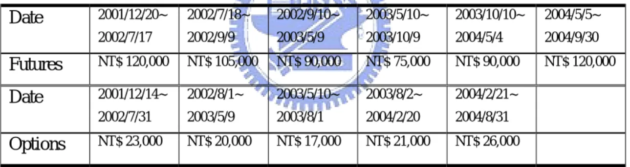
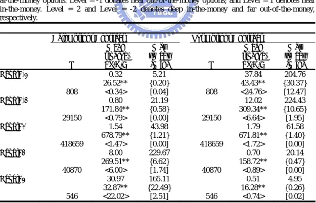
(26) index points for the sample period. When there is opportunity for unwinding, the trading costs for member arbitrageurs are (future price * 0.025% - settlement price * 0.025%) + 4*(call price * 0.125% + put price * 0.125% - settlement price * 0.025% * 0.25). Because the settlement costs have been considered at the initial trade, we save the settlement costs. The average unwinding trading costs for member arbitrageur are 0.32 index points for the sample period. For non-member arbitrageurs, the unwinding trading costs are (futures price * 0.025% - settlement price * 0.025%) + 4*(call price * 0.125% + put price * 0.125% - settlement price * 0.025% * 0.25) +4*(0.5). As described at section 3.2.2, the commissions for futures have been considered round trip fees at the initial. The average unwinding trading costs for nonmember arbitrageur are 2.48 index points for the sample period. The margin deposit per arbitrage portfolio is estimated to be between 630 and 835 index points. The initial margin for options and futures are shown at table 1. Table 1 The initial margin for futures and options 2001/12/20~. 2002/7/18~. 2002/9/10~. 2003/5/10~. 2003/10/10~. 2004/5/5~. 2002/7/17. 2002/9/9. 2003/5/9. 2003/10/9. 2004/5/4. 2004/9/30. Futures. NT$ 120,000. NT$ 105,000. NT$ 90,000. NT$ 75,000. NT$ 90,000. NT$ 120,000. Date. 2001/12/14~. 2002/8/1~. 2003/5/10~. 2003/8/2~. 2004/2/21~. 2002/7/31. 2003/5/9. 2003/8/1. 2004/2/20. 2004/8/31. NT$ 23,000. NT$ 20,000. NT$ 17,000. NT$ 21,000. NT$ 26,000. Date. Options. Since a put-call-futures arbitrage portfolio comprises of one futures position, one long and one short position in the options, we use table above to calculate total initial margin per arbitrage portfolio. The average interest cost for the margin deposit is estimated as 0.276 index points. The options are divided into five levels of moneyness5—from -2 to +2, where Level =0 indicates the at-the-money options. Level = -1 donates near out-of-the-money options; and Level = 1 denotes near in-the-money. Level = 2 and Level = -2 denotes deep in-the-money and far out-of-the-money, respectively. The percentage spread cost per transaction in the contracts is calculated 5. The fraction F/X is used to define moneyness because the asset that is hedged by the options contracts is the futures contract. At-the-money is defined as 0.95≦F/X≦1.05, near-the-money is defined as 0.85 ≦F/X<0.95 and 1.05<F/X≦1.15, and far-from-the-money is defined as F/X<0.85 and 1.15<F/X. 18.

(27) according to the following formula (see ap Gwilymm, Buckle & Thomas, 1997; Yadav & Pope, 1994): Percentage spread =. Ask −1 ( Ask + Bid ) / 2. For the options contract, we sort the contracts for any particular day into two different maturities: less than 30 days and greater than 30 days. For each maturity series, the contracts are further sorted according to the moneyness of the contract as mentioned above. Hence, we obtain ten different average percentage spreads for both the call and the put on each trading day. The one-way spread cost is equal to the price multiplied by the average percentage spread for the contract that belongs to the particular category. For futures contract, they are classified into two different categories as with the different maturities of option quotes. The one-way spread cost is equal to the futures price multiplied by the average percentage spread for the maturity subgroup for that particular day. Table 2 Spread costs for call options and put options, January 2002 – August 2004 The options are divided to five levels of moneyness—from -2 to +2, where Level =0 indicates the at-the-money options. Level = -1 donates near out-of-the-money options; and Level = 1 denotes near in-the-money. Level = 2 and Level = -2 denotes deep in-the-money and far out-of-the-money, respectively. Call Options Contract Put Options Contract Mean Max Mean (t-value) {Med} (t-value) N <S.D.> [Min] N <S.D.> 0.32 5.21 37.84 Level=-2 26.52** {0.20} 43.43** 808 <0.34> [0.04] 808 <24.76> 0.80 21.19 12.02 Level=-1 171.84** {0.58} 309.34** 29150 <0.79> [0.00] 29150 <6.64> 1.54 43.98 1.79 Level=0 678.79** {1.21} 671.81** 418659 <1.47> [0.00] 418659 <1.72> 8.00 229.67 0.70 Level=1 269.51** {6.62} 158.72** 40870 <6.00> [1.74] 40870 <0.89> 30.97 165.11 0.51 Level=2 32.87** {22.49} 16.28** 546 <22.02> [2.51] 546 <0.74> The statistical descriptions of spread cost are in index points. **Indicate statistical significance at the 0.01 level *Indicate statistical significance at the 0.05 level. Max {Med} [Min] 204.76 {30.37} [12.47] 224.43 {10.65} [1.95] 61.58 {1.40} [0.00] 20.14 {0.47} [0.00] 4.95 {0.26} [0.02]. Table 2 presents the spread cost for call options and put options for the matched 19.

(28) trios. Most of the trios occur at the moneyness of at-the-money. The spread cost is higher when the call and put options are deep in-the-money than if they are far out-of-the-money. The average spread cost of futures is estimated as 0.9 index points for the sample period.. 4.3 Empirical methodology for three-equation model The specific variables in three-equation model are calculated as below:. Biast = F0 − F * , where F0* is defined in equation (1). Spread t equals best ask price minus best bid price. Deptht equals the quantity of best bid price plus the quantity of best ask price. VALt equals the average of implied volatility of matched call and put options.. To mitigate the econometric problems, all variables in Equation (15) through (17) were transformed into log form. This enabled us to stabilize the variance of the error terms and approximate error terms toward a symmetric distribution. In addition, to avoid any spurious relationship among the variables because of the presence of a unit root in the time series, we applied the augmented Dickey-Fuller test (ADF) to test for differenced stationary. Results from ADF tests indicate that only ln( FPt ) term should be estimated in first difference form. The GMM procedure, an instrumental variable method suggest by Hansen (1982), was used to estimate the parameters of our three-equation model. The merit of this procedure is that it provides a set of consistent estimates of parameters as well as corresponding standard errors for each of the parameter estimates under serially correlated and heteroskedastic error terms of our simultaneous equations model.. 20.

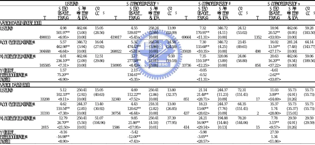
(29) 5. Empirical results 5.1 Ex-post simulations Tables 6 and 7 summarize the distribution of the ex-post pricing errors inferred from the transaction prices and the bid/ask quotes, respectively. Table 6 comprises four panels. Panel A (the zero-spread cost category) shows the distribution without adjusting for the bid and ask spread of the contracts. Panel B (the zero-transaction-cost category) adjusts for bid and ask spreads. Panel C (the member cost category) adjusts for bid and ask spreads as well as the exchange trading fees against members, and Panel D (the non-member cost category) adjusts for bid and ask spreads, exchange trading fees, and commissions. Table 7 excludes the zero-spread cost category, since the spread cost is implicit in the calculation with the bid/ask quotes data. The following tables are also classified according to Table 6 and 7.. 5.1.1 Frequency of potential arbitrage opportunities. The frequency of potential arbitrage opportunities declines with increases in the trading costs and margin requirements. For the transaction price data (Table 6), the number of mispriced observations declines from 490,033 to 33,208 after factoring in the spread costs for the contracts. The 7,421 and 1,583 mispricings are for members and non-members, respectively. From the bid/ask quote signals, 60,067 and 7,165 mispricings are for member and non-member cost category, repectivley(Table 7). These matched trios are located around the most liquid at-the-money options. This is consistent with previous studies. The number of no-arbitrage violations based on bid/ask quotes is larger than those that are signaled by transaction prices.. 5.1.2 The magnitude of arbitrage profit. Based on transaction price, the average ex-post arbitrage profit inferred from zero spread cost data is 4.98 index points and the long-futures strategy is not necessarily more profitable and more frequent than short-futures strategy. The result is 21.

(30) inconsistent with Klemkosky and Lee (1991) and Fung and Mok (2001), but the same with that of Fung and Fung (1997).. Moreover, the standard deviations of. short-futures strategies are greater than those of long-futures strategies. The mean profits for non-members is higher (17.41) than that of members (8.05). The result is different from that of Fung and Fung (1997) and Marchand, Lindley, and Followill (1994) shows that profitable trading opportunities only for those traders with lowest transaction cost. However, the result is the same as Fung and Mok (2001). Fung and Mok (2001) interpret higher average profit for non-members are because the higher cost threshold of for non-members, the test picked out the far right side of the error distribution. Therefore, the mean and median profits for non-members are both higher than that of the other cost filters. However, the 95 and 99 percentile observations show that the results may be attributable to a few extreme values. Based on bid/ask quotes (Table 7), the average potential profit for non-members is also higher (7.94 index points) than that of the members (4.56 index points) and the benchmark group of zero-transaction-cost arbitrageurs (4.08 index points). However, in comparison with the results derived from transaction prices (Table 2), the reduction in arbitrage profit is apparent. We can discuss the results in two sides: On one hand, the result of reduced profit is inconsistent with Fung and Mok (2001). They propose that the profit based on bid/ask quotes is more profitable. But, this finding is the same as that of Bae, Chan, and Cheung (1998). They find that arbitrage profit based on transaction prices can be overstated because of bases in evaluating arbitrage profitability based on transaction prices. However, the 95 and 99 percentile based on transaction price show that extreme values are less frequent than that of bid/ask quotes. The maximum profit based on bid/ask quotes is larger than that of transaction prices. This implies that if profitable bid/ask quotes could be executed immediately, the chance of earning extreme arbitrage profits could be enhanced. On the other hand, the result of overstated arbitrage frequencies based on bid/ask quotes is consistent with that of Fung and Mok (2001). They consider that bid/ask quotes can provide more potential information than transaction prices. As a result, the violations of on-arbitrage band based on bid/ask quotes can be viewed as arbitrage signals. However, this finding differs from that of Bae, Chan, and Cheung (1998).. 22.

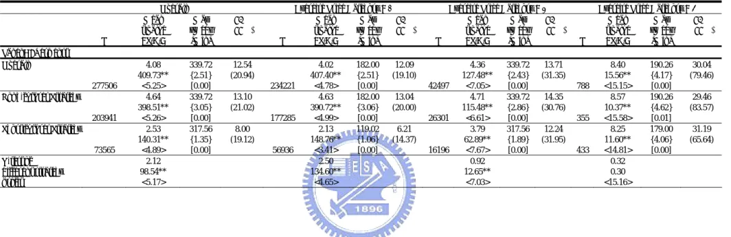
(31) 5.2 Ex-ante simulations. Tables 8 and 9 demonstrate that arbitrage trade which is taken into consideration possible execution time lags from the transaction prices and the bid/ask quotes, respectively.. 5.2.1 Ex-ante simulations of transaction prices. Table 8 shows the ex-ante simulated arbitrage profit from an execute-and-hold strategy (Klemkosky & Lee, 1991). Across all categories of lags, arbitrage trades are significantly profitable only if the transactions are executed with a 3-min time lag for zero spread cost group (3.59 index points) and zero transaction cost group (1.91 index points). However, when the time lag increases to more than 3-min, the magnitude of the arbitrage profit decrease substantially. The majority of the ex-ante opportunities is also concentrated in 3-min time lag, over 85 percent of ex-ante trades is profitable for zero-transaction cost group and members. This implies that the number of mispricing opportunities that last longer than 3 min becomes small and arbitrageurs with lower cost threshold (zero-transaction cost group and members) could have chance of over 50% to obtain positive profits as soon as their trades are executed immediately. Furthermore, the results suggest a negative relationship between the magnitude of arbitrage profit and the execution time lag and indicate that the market is dynamically efficient with price adjustments to correct for pricing errors completed in less that 3 min. Comparing profitability between the long-future arbitrage opportunities and the short-future arbitrage opportunities, we find that, the ex-ante average long-future arbitrage opportunities with zero cost assumed are marginally more profitable and more frequent than short-futures opportunities (4.28 and 304,449 for long futures & 1.86 and 185,584 for short futures). The profit for short-futures strategy becomes negative after factoring in costs. However, arbitrageurs with zero transaction cost threshold could obtain significant profits from long-futures signals. And the risk of extreme lost for long-futures signals is relatively higher.. 5.2.2 Ex-ante simulations of bid/ask quotes. 23.

(32) The ex-ante arbitrage profits based on bid/ask quotes also decline quickly and disappear within three minutes. Table 9 shows that for non-members, the median of arbitrage profits is positive within lag 3-min category. This indicates that non-members arbitrageurs could obtain profitable trading based on bid/ask arbitrage signals more than that of transaction prices. Again, this dynamic adjustment of the price errors based on bid/ask quotes is consistent with the dynamic efficiency of the options-futures markets. For a time lapse of less than three minutes, Table 9 shows that both the frequency and size of profitable arbitrage opportunities and the magnitude of arbitrage profits for members and non-members inferred from bid/ask quotes are larger than those simulated from transaction prices that we see in Table 8. Fung and Mok (2001) explain that scenes could be a result of stale price, transaction prices understate both the frequency and size of arbitrage opportunities than that are inferred from bid/ask quotes. Table 10 provides further evidence of stale prices and execution delay of the bid/ask quotes. In Table 10, we match the nearest actual transaction to a detected profitable mispricing signal based on the bid/ask quotes. It is apparent that all the average ex-ante arbitrage profits are negative. The result is identical to Fung and Mok (2001). This implies that the market makers may be able to eliminate the arbitrage profit to the counterparty. The market-making system does not display systematic pricing errors.. 5.3 Regression analysis Table 3 displays the effect of execution delay on the change in the potential arbitrage profit. As expected, the change in arbitrage profitability ( eT ,t − eBA,t ) is negatively and significantly related to the four determinants for all arbitrageur groups. However, the most interesting thing is the positive intercept term. That means arbitrage trade follows the arbitrage signal based on the bid/ask quotes and execute at transaction price will guarantee positively extra profits, ceteris paribus. The crucial factors we consider are the negative coefficients of execution risk (σ t ) and execution delay ( Lt ) . The lower the execution risk proxy (σ t ) , the less negative (eT ,t − eBA,t ) is, ceteris paribus. Also, if we shorten the time gap ( Lt ) 24.

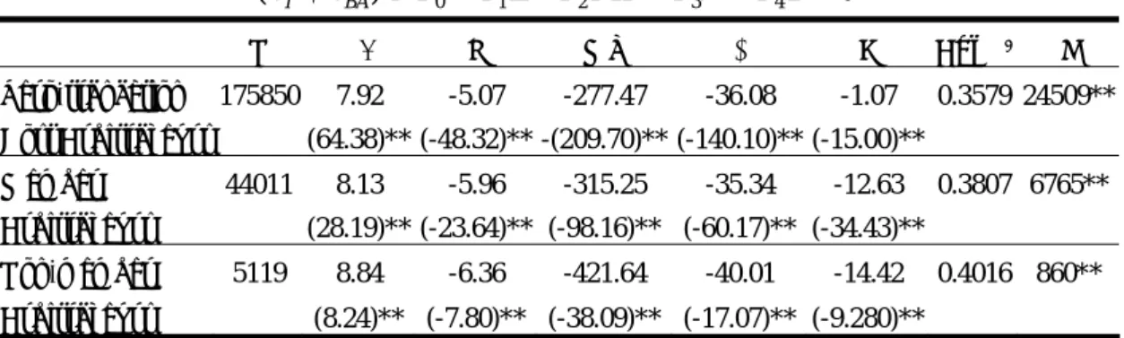
(33) between detecting a profitable bid/ask signal and executing the quotes, the arbitrage profit derived from transaction prices would close to that of the bid/ask quotes. That is, the value of ( eT ,t − eBA,t ) increase, meaning higher arbitrage profit. The implication is that the practitioners can enhance their arbitrage profit by reducing the execution delay between detecting a profitable bid/ask signal and executing the quotes. As we notice from table 3, the most negative term is moneyness of the arbitrage portfolio. That is, when arbitrageurs trade far-from-the-money portfolio, they might lost a lot. And using the long-futures strategy can align closer the change of profit. As a result, the profit can be enhanced after controlling for the degree of moneyness and the type of hedging strategy. Regression results suggest that the bid/ask quotes provide valuable trading signals to the arbitrageurs. The arbitrageurs could enhance their put-call-futures arbitrage profits by exploiting information from the bid/ask signals, lowering the execution risk, reducing the execution delay, trading near-the-money portfolio and adopting the long-futures strategy. Table 3 Regression analysis on put-call-futures arbitrage for the difference between the bid/ask quoted data and the transaction price with adjust for spread cost The following regression model is used to assess the impact of execution delay on the change in the potential arbitrage profit. Where, ( eT − e BA ) equals the change in potential profitability derived from transaction prices and that inferred form bid/ask quotes, L equals the execution delay between detecting a profitable bid/ask signal and executing the quotes, σ equals futures price volatility, MY equals the moneyness of the options used in the arbitrage ( MY = (| X − F0 | / X ) ), D equals the type of arbitrage strategies, D = 0 for a long-futures strategy; and strategy.. D = 1 for the short-futures. ( eT − eBA ) = α 0 + α1 L + α 2 MY + α 3σ + α 4 D + ε Zero-tranaction. N. α0. L. MY. σ. D. 175850. 7.92. -5.07. -277.47. -36.08. -1.07. Cost Arbitrageurs Member. F. 0.3579 24509**. (64.38)** (-48.32)** -(209.70)** (-140.10)** (-15.00)** 44011. Arbitrageurs Non-member. Adj R2. 8.13. -5.96. -315.25. -35.34. -12.63. 0.3807 6765**. (28.19)** (-23.64)** (-98.16)** (-60.17)** (-34.43)** 5119. 8.84. -6.36. -421.64. -40.01. -14.42. (8.24)** (-7.80)** (-38.09)** (-17.07)** (-9.280)** Arbitrageurs t statistics are in parentheses. **Indicate statistical significance at the 0.01 level *Indicate statistical significance at the 0.05 level. 25. 0.4016 860**.

(34) 5.4 Early-unwinding strategy with transaction prices and bid/ask quotes By assuming that trades can be executed at the prevailing quotes, the early unwinding strategy adds extra profit to all arbitrage groups over and above that of the hold-to-expiration strategy (Tables 11 and 12 ). The total (equals initial plus incremental). early-unwinding. profits. (4.08+3.15,. 4.59+12.73,. 7.56+28.59,. respectively.) for the three classes of investor (Table 12) are smaller than the same categories derived from transaction prices (Table 11). The results are the same as previous hold-to-expiration strategy. The average profit for same-day unwinding which derived from transaction prices is higher than unwinding the positions in other days except zero spread cost group(Table 11), yet the outcome of the bid/ask quotes is the inverse except members groups(Table 12). However, the short-futures strategy for the both tables shows that the average profit for same-day unwinding is lower than unwinding the positions in other days. Results indicate that the holding period for arbitrage trades is long. In addition, the trades incorporate higher transaction costs in the beginning, trader can save settlement fees and margin deposits when unwinding. As a result, the average unwinding profit for member and nonmember arbitrageur is larger than initial profit.. 5.5 Early-unwinding and hold-to-expiration strategies From table 4, it is easy to tell the difference between early-unwinding and hold-to-expiration strategies. Results show that when arbitrageurs execute trades at prevailing bid/ask quotes, size of arbitrage profit are smaller than that signaled by transaction data under either the early-unwinding or the hold-to-expiration strategy. But, the frequency of arbitrage trades is the inverse. Note that t-test shows there is significantly extra profit from hold-to-expiration to early-unwinding strategy. The extra profits are almost larger than average profits of hold-to-expiration strategy, excluding that based on bid/ask quotes with zero-cost arbitrageurs. And nearly over 80% trades based on bid/ask quotes and transaction price can be unwound before maturity, except nonmember arbitrageurs (76% and 59%, respectively). In general, the total arbitrage profit derived from early unwinding of the initial 26.

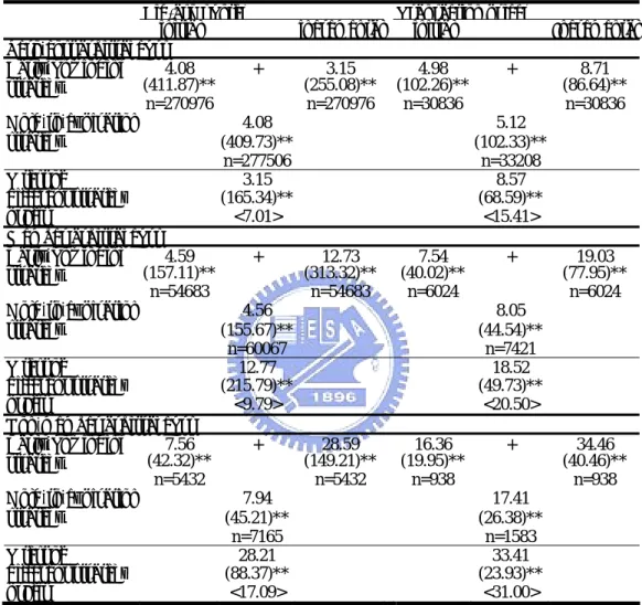
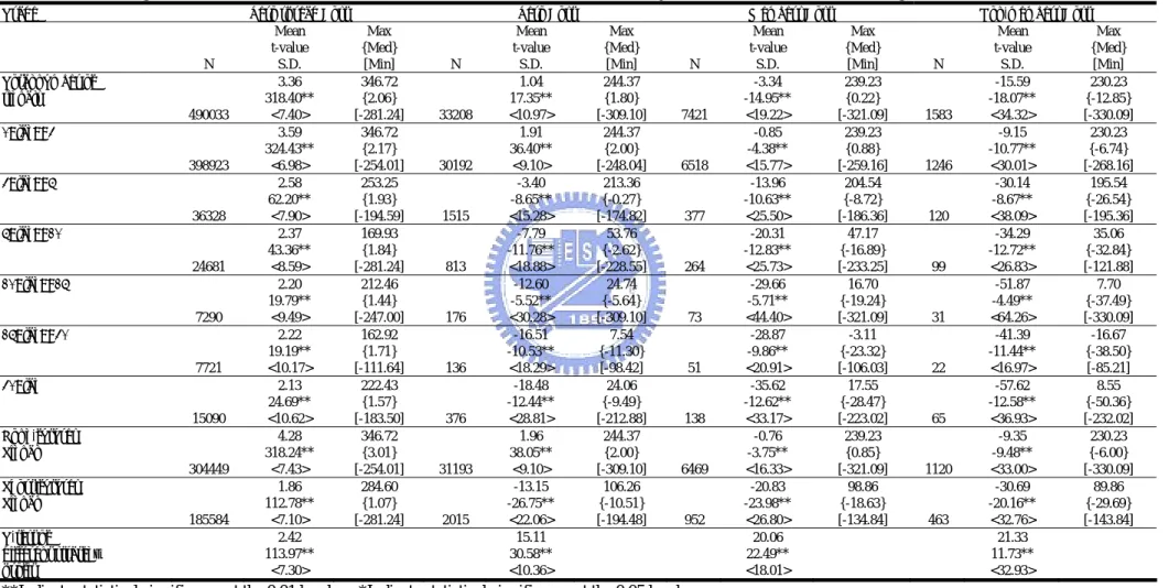
(35) arbitrage portfolio based on transaction price is the highest. Second highest profits are generated by the early-unwinding profit derived form bid/ask quotes, followed by the hold-to-expiration. strategy. with. transaction. prices,. and. lastly,. the. static. hold-to-expiration strategy with bid/ask quotes. Table 4 Average profit of the early-unwinding and hold-to-expiration strategies Bid/ask quotes Transaction prices initial incremental initial Incremental Zero-cost arbitrageurs + + 4.08 3.15 4.98 8.71 Early-unwinding (411.87)** (255.08)** (102.26)** (86.64)** strategy n=270976 n=270976 n=30836 n=30836 4.08 5.12 Hold-to-expiration strategy (409.73)** (102.33)** n=277506 n=33208 3.15 8.57 T test of (165.34)** (68.59)** different strategy <7.01> <15.41> profit Member arbitrageurs + + 4.59 12.73 7.54 19.03 Early-unwinding (157.11)** (313.32)** (40.02)** (77.95)** strategy n=54683 n=54683 n=6024 n=6024 4.56 8.05 Hold-to-expiration strategy (155.67)** (44.54)** n=60067 n=7421 12.77 18.52 T test of (215.79)** (49.73)** different strategy <9.79> <20.50> profit Non-member arbitrageurs + + 7.56 28.59 16.36 34.46 Early-unwinding (42.32)** (149.21)** (19.95)** (40.46)** strategy n=5432 n=5432 n=938 n=938 7.94 17.41 Hold-to-expiration strategy (45.21)** (26.38)** n=7165 n=1583 28.21 33.41 T test of (88.37)** (23.93)** different strategy <17.09> <31.00> profit Figures for the hold-to-expiration strategy are reproduced from Table 2 and 3. Figures for the early-unwinding strategies are reproduced from Table 8 and 9. t statistics are in parentheses. Total arbitrage profit from early unwinding is the sum of the initial profit based on the static hold-to-expiration strategy and the incremental profit from early unwinding. **Indicate statistical significance at the 0.01 level *Indicate statistical significance at the 0.05 level. 27.

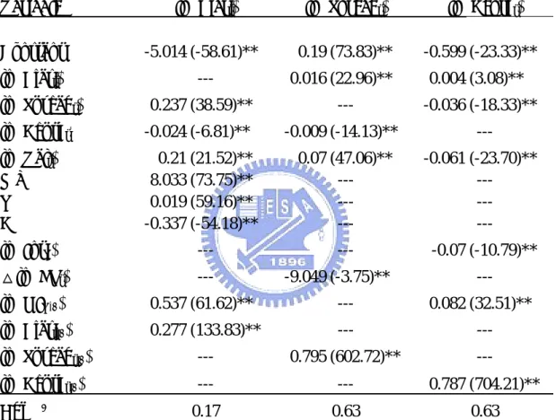
(36) 5.6 The empirical results for three equation model In Table 5, the GMM estimation result shows that mispricing, spread and market depth are all endogenous variables and simultaneously determined in the system. And other properties are also described as following. Table 5 Empirical Results on the Mispricing, Bid-Ask Spread and Market depth Equations of TAIFEX Index Futures from January 2, 2002 to August 31, 2004 Variable. ln (Biast). ln (Spreadt). ln (Deptht). Constant. -5.014 (-58.61)**. 0.19 (73.83)**. -0.599 (-23.33)**. ln (Biast). ---. 0.016 (22.96)**. 0.004 (3.08)**. ln (Spreadt). 0.237 (38.59)**. ---. -0.036 (-18.33)**. ln (Deptht). -0.024 (-6.81)**. -0.009 (-14.13)**. ---. ln (Valt) MY T D. 0.21 (21.52)** 8.033 (73.75)** 0.019 (59.16)** -0.337 (-54.18)**. 0.07 (47.06)** -------. -0.061 (-23.70)** -------. ln (IntT). ---. ---. -0.07 (-10.79)**. △ln (FPt). ---. ln (OIT-1). 0.537 (61.62)**. ---. 0.082 (32.51)**. ln (Biast-1). 0.277 (133.83)**. ---. ---. ln (Spreadt-1). ---. 0.795 (602.72)**. ---. ln (Deptht-1). ---. ---. 0.787 (704.21)**. 0.17. 0.63. 0.63. Adj R2. -9.049 (-3.75)**. ---. 1. Where Bias t is the mispricing at the tth moment. Biast −1 is Bias t lagged moment;. Spread t is the bid-ask spread at the tth moment. Spread t −1 is Spread t lagged moment; Deptht is the sum of quantity of best bid and ask at the tth moment. Deptht −1 is Deptht lagged moment; VALt is average of implied volatility of call and put at the tth moment. VALt −1 is VALt lagged moment; OI T −1 is the open interest on the Tth day lagged 1 day; IntT is the one-month time deposit of the postal savings system on the Tth day; FPt is the future transaction price at the tth moment; T is the time to maturity of the contract; D is the dummy variable to reflect differences for arbitrage signal, D =1 is short strategy signal, D =0 is long strategy signal. 2. All variables are transformed into log form. 3. Each equation is estimated by the generalized method of moment (GMM). 4. Numbers in parentheses are t statistics. 5. △ denotes the first difference operator. **Indicate statistical significance at the 0.01 level 28.

(37) 5.6.1 Bias Equation. Results of the Bias equation are presented in Column 2 of Table 5. The coefficient of Spread was positively related to Bias and statistically significant at the 1% level. The Spread represents the intraday liquidity component. This finding can be interpreted that an increase in liquidity will reduce mispricing, ceteris paribus. Result shows that Depth was negatively related to Bias and statistically significant at the 1% level. The Depth represents the information component. Arbitrageurs use the arbitrage message to submit orders and cause the mispricing magnitude to reduce. This means the arbitrage mechanism was really efficient in Taiwan options and futures market. However, the lagged OI represent past information component. Result shows that it was positively related to Bias. It means lagged OI would disturb the market price. As expected, the coefficient of volatility (Val) was positive. When traders face great uncertainty or risk, the fundamental price would be uneasy to agree with. Thus, the mispricing would be enhanced. The three variables (MY, T, D) indicate the mispricing often occurs in what situation. Results point out when trading far-from-the-money portfolio, the contracts have long time to expire and the Bias is negative sign (D=0), the degree of mispricing is relatively large. However, the most crucial variable is the degree of moneyness. The coefficient of lagged Bias was positively related to Bias. The significant persistence of mispricing was consistent with first category in Table 8. But, the Bias will be eliminated after 3 minutes when incorporate transaction costs.. 5.6.2 Spread Equation. Coefficient estimates of the explanatory variables on the Spread equation are presented in column 3 of Table 5. The coefficient of Bias was significantly positive related to Spread. As informed traders notice the obvious mispricing, they would take advantage of arbitrage signals. However, market maker must increase the Spread to compensate for expected losses when trading opposite to informed traders. The Spread will be enhanced 0.19% as Bias increase 1%. The coefficient of Depth was negative and statistically significant at the 1% level. This result is similar with that of previous studies; trading activity is inversely related 29.