行政院國家科學委員會專題研究計畫 成果報告
H.264 之轉換編碼及最佳化
計畫類別: 個別型計畫
計畫編號: NSC93-2213-E-002-137-
執行期間: 93 年 10 月 01 日至 94 年 07 月 31 日
執行單位: 國立臺灣大學電信工程學研究所
計畫主持人: 陳宏銘
報告類型: 精簡報告
報告附件: 出席國際會議研究心得報告及發表論文
處理方式: 本計畫可公開查詢
中 華 民 國 94 年 8 月 25 日
行政院國家科學委員會補助專題研究計畫
■ 成 果 報 告
□期中進度報告
Transcoding and Optimization of H.264
計畫類別:▓ 個別型計畫 □ 整合型計畫
計畫編號:NSC 93-2213-E-002-137-
執行期間: 93年10月 日至 94年07月 日
計畫主持人:陳宏銘
共同主持人:
計畫參與人員: 陳宸、林樹法、張哲瑜、吳秉浩、呂孟庭、蘇哲群、林亦倫
成果報告類型(依經費核定清單規定繳交):▓精簡報告 □完整報告
本成果報告包括以下應繳交之附件:
□赴國外出差或研習心得報告一份
□赴大陸地區出差或研習心得報告一份
▓出席國際學術會議心得報告及發表之論文各一份
□國際合作研究計畫國外研究報告書一份
處理方式:除產學合作研究計畫、提升產業技術及人才培育研究計畫、列管計畫
及下列情形者外,得立即公開查詢
□涉及專利或其他智慧財產權,□一年□二年後可公開查詢
執行單位:國立台灣大學電信工程學研究所
中 華 民 國 94 年 8 月 日
摘要
本計畫以先前自行開發的研究成果為基礎,繼續探討MPEG-2至H.264之轉換編碼架構。此轉換
編碼器的功能是將視訊轉換至H.264格式,並將影像解析度降至原來的一半。在此架構中,我們將轉
換核心變換 (transform kernel conversion, 亦即從MPEG-2之離散餘弦轉換至H.264之近似離散餘弦)之
計算合併至降採樣(down sampling)的程序中。對Intra frame的轉換編碼,我們探討DCT-to-PEL和
DCT-to-DCT兩種轉換編碼架構。相形之下,DCT-to-PEL之運算較簡單。然而DCT-to-DCT的intra frame
轉換編碼尚未有人做過,我們是第一個完成理論性探討的研究單位。對inter frame的轉換編碼我們則
採用DCT-to-DCT之轉換編碼架構,盡量避開完全解碼再重新編碼的轉換編碼工作,減少運算量。
本計畫的另一目標為H.264最佳化,針對移動估測和模式選擇兩項關鍵模組,繼續研究簡化運算
量之方法。在移動估測方面發展可調變式搜尋策略 (包括動態移動向量預估器、提前終止,與動態搜
尋樣式) 與動態多重參考畫面選擇技術,將編碼速度增為原本參考軟體 (JM 8.5) 的六倍左右。在模式
選擇方面,利用方塊模式在空間與時間上的相關性,發展快速模式選擇演算法,將編碼速度提升約
兩倍左右。整合這兩種快速演算法於編碼器中,總編碼速度增加約十二倍,而編碼效能仍維持在原
來的程度,僅受非常輕微影響。
關鍵詞:H.264、MPEG-4、H.263、離散餘弦轉換、轉換編碼器、降採樣、多重方塊大小、移動估
測、模式選擇、多重參考畫面
Abstract
A key objective of this project is to develop a transcoder for converting an MPEG-2 video bitstream to
the H.264 format. Along with the conversion, we also reduce the image resolution by half in each dimension.
For computational efficiency, we avoid full decompression and full recompression in the spatial domain. The
output bitstream is fully compliant to the H.264 standard. In our technique, the "transform conversion"
between the DCT of MPEG-2 and the modified DCT of H.264 is incorporated in the down-sampling process.
Inter and intra frames are processed separately. For transcoding of intra frames, both DCT-to-PEL and
DCT-to-DCT architectures are considered, while for inter frames a DCT-to-DCT architecture is adopted.
Another objective of this project is to improve the computational efficiency of two core modules, motion
estimation and mode decision, of H.264. For motion estimation, we develop a fast algorithm with adaptive
search strategy and intelligent reference frame selection. Compared with the H.264 reference software JM
8.5, this algorithm achieves, on the average, a 600% reduction of encoding time. For mode decision, we
exploit the correlation between neighboring image blocks to predict the best possible mode. Compared with
the reference software, this method achieves about 204% reduction of encoding time with negligible PSNR
drop and bit rate increase. Integrating these two fast algorithms in the H.264 reference software, this
combined method, on the average, is about 12.1 times faster in the total encoding time, at the cost of a slight
PSNR drop.
Keywords:
H.264, MPEG-4, H.263, DCT, transcoding, down-sampling, variable block-size, motion
estimation, mode decision, multiple reference frames
Contents
I. INTRODUCTION...1
A. MPEG-2 to H.264 Transcoding ...1
B. Optimization of H.264 ...1
II. Transcoding and Downsampling...1
A. Transcoding of I-Pictures...1
B. Transcoding of P-Pictures ...2
1) Down-Sampling and Transform Conversion ...2
2) Fast
Computations...3
III. Transform-Domain Intra Prediction...4
IV. Optimization of H.264 ...4
A. Fast
Mode
Decision ...4
1) Analysis...5
2) Algorithm
Description ...6
B. Fast Motion Estimation ...7
1) Adaptive
Search
Strategy...7
2) Flexible Multi-Frame Search Scheme...9
3) Architecture of Combined Algorithm ...10
V. Simulation
Results ...10
A. Transcoding
and
Downsampling...10
B. Optimization of H.264 ...10
1) Fast Mode Decision ...10
2) Fast Multi-Frame Motion Estimation ...11
3) Combined
Algorithm ...11
VI. Achievements ...12
A. Publications ...12
B. Patents ...12
I. INTRODUCTION
A. MPEG-2 to H.264 Transcoding
In the context of MPEG-2 to H.264 transcoding, the issues to be addressed include macroblock mode selection, motion vector determination, transform kernel conversion, transform block size conversion, and transform-domain intra prediction.
In macroblock mode selection, the four macroblocks to be converted to one may have different modes. Based on the four modes, a best mode has to be determined for the down-sampled macroblock. Our approach, in order to save the computational cost, is to simply assign the inter mode to the resulting macroblock if the four original macroblocks are not of the same mode, instead of carrying out a new macroblock mode decision process.
Likewise, the motion vectors of the four original macroblocks may be different. Simply converting the four motion vectors to one by averaging does not work well in practice. In our work, we consider the advanced prediction mode supported in H.264 that allows one motion vector per 8 x 8 luminance block. Under this mode, the motion vector of a 16 x 16 macroblock is scaled down by a factor of 2 and assigned to the down-sampled 8 x 8 block.
The down-sampling process is performed in the DCT-domain, like that in [2]. However, the problem we deal with here demands a new treatment because H.264 and MPEG-2 have different transform kernels and transform block sizes. The block size used for transform and quantization in H.264 is 4 x 4, while the block size is 8 x 8 in MPEG-2. In addition, H.264 uses a modified DCT, which is different from the conventional DCT in MPEG-2. Our goal is to solve these problems without introducing additional computational cost.
B. Optimization of H.264
H.264/AVC [1], which will play an important role in multimedia communications and consumer electronics applications, is a new international video coding standard jointly developed by the ITU-T Video Coding Experts Group and the ISO/IEC Moving Picture Experts Group. It achieves higher coding efficiency than that of previous standards such as MPEG-2 and H.263. However, the coding gain comes at the cost of a much higher computational complexity. For practical purposes, there is a need for reducing the computational complexity of H.264.
The increase of the computational cost of H.264 is largely due to the use of variable block-size motion estimation (ME), multiple reference frames, and rate-distortion (R-D) optimized mode decision (MD). Like previous video coding standards, H.264/AVC employs motion estimation/compensation to remove temporal redundancy between frames. However, the size of a block in H.264 can be 16x16, 16x8, 8x16, 8x8, 8x4, 4x8, or 4x4 [1]. The number of possible modes that an encoder has to examine is significantly increased since each block size leads to a different mode. Our run time analysis of the H.264 reference software indicates that ME and MD consume about 90% of the total encoding time (for either 1 or 5 reference
frames). Therefore, these two modules are the main target of complexity reduction in our work.
We develop fast multi-frame motion estimation and mode decision algorithms which reduce the computational complexity of H.264 encoders. For MD, we develop a fast algorithm by exploiting the mode distribution and the mode similarity of neighboring macroblocks to reduce the computational load. The most information used in our mode decision method, such as the modes of neighboring macroblocks, is already available in the encoding processes. For ME, we develop a fast multi-frame motion estimation algorithm with an adaptive search strategy and a flexible multi-frame search scheme. The core of our adaptive search strategy is formed by a combination of motion prediction, adaptive early termination, and dynamic search pattern to maintain the coding efficiency and reduce the computational cost. Our multi-frame search scheme increases the search efficiency by skipping unnecessary reference frames.
II. TRANSCODING AND DOWNSAMPLING
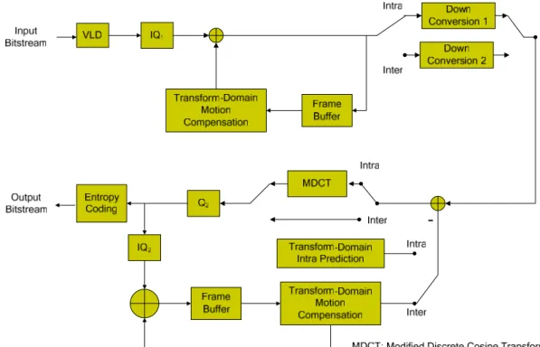
The architecture of the proposed transcoder is depicted in Figure 1, where the switches control the intra/inter decision. The input of the transcoder is a full resolution MPEG-2 video bitstream, and the output is a half resolution H.264 video bitstream.
Recall that every four 16 x 16 macroblocks (total size 32 x 32) in the original picture are converted into one 16 x 16 macroblock in our method. In the following, we describe how the down-sampling process works. Here, upper case letter is used to represent a block of DCT coefficients, and lower case letter is used to represent a block of pixel values.
A. Transcoding of I-Pictures
We start with the transcoding of I-pictures. In our approach, the down-sampling process of I-pictures is combined with IDCT. Both down-sampling and transform are represented by matrix multiplications in the following discusison.
Let xi, i = 1…4, be the four 8x8 blocks before
down-sampling and y the 8x8 block after down-sampling. The down-sampling operation (a simple 2 x 2 averaging filter) can be represented in the matrix form
1 1 1 1 2 2 2 3 1 2 4 2 1 4 t t t t
y =
(
q x q + q x q + q x q + q x q
),
(1) where 1 1 1 0 0 0 0 0 0 0 0 1 1 0 0 0 0 0 0 0 0 1 1 0 0 0 0 0 0 0 0 1 1 0 0 0 0 0 0 0 0 0 0 0 0 0 0 0 0 0 0 0 0 0 0 0 0 0 0 0 0 0 0 0 0 ⎡ ⎤ ⎢ ⎥ ⎢ ⎥ ⎢ ⎥ ⎢ ⎥ = ⎢ ⎥ ⎢ ⎥ ⎢ ⎥ ⎢ ⎥ ⎣ ⎦ q (2) and2 0 0 0 0 0 0 0 0 0 0 0 0 0 0 0 0 0 0 0 0 0 0 0 0 0 0 0 0 0 0 0 0 1 1 0 0 0 0 0 0 0 0 1 1 0 0 0 0 0 0 0 0 1 1 0 0 0 0 0 0 0 0 1 1 . ⎡ ⎤ ⎢ ⎥ ⎢ ⎥ ⎢ ⎥ ⎢ ⎥ = ⎢ ⎥ ⎢ ⎥ ⎢ ⎥ ⎢ ⎥ ⎣ ⎦ q (3)
Denote the eight-point DCT matrix by S, with
,
7
,
0
16
1
2
cos
2
)
(
)
,
(
⎟
≤
≤
⎠
⎞
⎜
⎝
⎛
+
⋅
=
c
i
j
i
i
j
j
i
s
π
,
(4) and⎩
⎨
⎧
=
=
.
1,
0
,
2
1
)
(
otherwise
i
i
c
(5)Then we can write the DCT operation of in the following matrix form
.
= t
X SxS (6) Therefore, (1) can be rewritten as
(
1 4 = t t + t t + 1 1 1 1 2 2 y q S X Sq q S X Sq)
. + t t t t 2 3 1 2 4 2 q S X Sq q S X Sq (7) Note that the matricesq S
1 t,q S
2 t,Sq
1t, andSq
2t can be pre-computed to save computations.B. Transcoding of P-Pictures
For the transcoding of P-pictures, we first describe the process of down-sampling and transform conversion. Then the motion vector mapping scheme we adopted is discussed. Finally, motion compensation in the transform domain is presented.
1) Down-Sampling and Transform Conversion
Because the 4 x 4 modified DCT is used in H.264, we need to convert an 8 x 8 block of conventional DCT coefficients into four 4 x 4 blocks of modified DCT coefficients. In our transcoder, the transform conversion and the down-sampling process is performed together in one operation in order to save computations.
Let X1, X2, X3, and X4 denote the four 8 x 8 blocks of DCT coefficients before down-sampling. We want to obtain a new 8 x 8 block Y, which consists of four 4 x 4 blocks of modified DCT coefficients.
Let us begin our derivation in the spatial domain. The new block y in the spatial domain can be obtained from X1, X2, X3, and X4 as follows
(
)
1 4 = t+ t + t + t 1 1 1 1 2 2 2 3 1 2 4 2 y q x q q x q q x q q x q 1 4( = t t + t t + 1 1 1 1 2 2 q S X Sq q S X Sq ). + t t t t 2 3 1 2 4 2 q S X Sq q S X Sq (8) Because the block size of the modified DCT transform in H.264 is 4 x 4, we divide y into four sub-blocks xi, i = 1…4. Then, the modified DCT is applied to each 4 x 4 sub-block. LetT be the transform matrix for a 4 x 4 modified DCT,
0 5 0 5 0 5 0 5 2 1 1 2 5 10 10 5 0 5 0 5 0 5 0 5 1 2 2 1 10 5 5 10 . . . . . . . . . ⎡ ⎤ ⎢ − − ⎥ ⎢ ⎥ = ⎢ − − ⎥ ⎢ ⎥ ⎢ − − ⎥ ⎣ ⎦ T (9)
Then the modified DCT transform of xi can be written as
. ⎡ ⎤ ⎡ ⎤ = ⎢ ⎥ ⎢ ⎥ ⎣ ⎦ ⎢⎣ ⎥⎦ ⎡ ⎤ ⎡ ⎤ ⎡ ⎤ =⎢ ⎥⎢ ⎥⎢ ⎥ ⎣ ⎦ ⎣ ⎦ ⎢⎣ ⎥⎦ ⎡ ⎤ ⎡ ⎤ =⎢ ⎥ ⎢ ⎥ ⎣ ⎦ ⎢⎣ ⎥⎦ t t 1 2 1 2 t t 3 4 3 4 t 1 2 t 3 4 t t X X Tx T Tx T X X Tx T Tx T x x T 0 T 0 x x 0 T 0 T T 0 T 0 x 0 T 0 T (10)
Therefore, we can perform the 4 x 4 modified DCT on the four sub-blocks of y using ⎡⎢ ⎤⎥ ⎣ ⎦ T 0 0 T and ⎡ ⎤ ⎢ ⎥ ⎢ ⎥ ⎣ ⎦ t t T 0 0 T . Applying this operation to (8) yields: 1 1 1 1 4 t t t t t t ⎡ ⎤ ⎡ ⎤ =⎢ ⎥ ⎢ ⎥ ⎣ ⎦ ⎢⎣ ⎥⎦ ⎡ ⎤ ⎡ ⎤ = ⎢ ⎥ ⎢ ⎥+ ⎣ ⎦ ⎢⎣ ⎥⎦ ⎡ ⎤ ⎡ ⎤ + ⎢ ⎥ ⎢ ⎥ ⎣ ⎦ ⎢⎣ ⎥⎦ ⎡ ⎤ ⎡ ⎤ + ⎢ ⎥ ⎢ ⎥ ⎣ ⎦ ⎢⎣ ⎥⎦ ( t t t 1 2 2 t t t t 2 3 1 t T 0 T 0 Y y 0 T 0 T T 0 T 0 q S X Sq 0 T 0 T T 0 T 0 q S X Sq 0 T 0 T T 0 T 0 q S X Sq 0 T 0 T 2 4 2 t t t t ⎡ ⎤ ⎡ ⎤ ⎢ ⎥ ⎢ ⎥ ⎣ ⎦ ⎢⎣ ⎥⎦), T 0 T 0 q S X Sq 0 T 0 T (11)
which can be rewritten as: 1 4 = ( 1 1 1t + 1 2 2t+ Y U X U U X U + ), t t 2 3 1 2 4 2 U X U U X U (12) where ⎡ ⎤ = ⎢⎣ ⎥⎦ t 1 1 T 0 U q S 0 T and . ⎡ ⎤ = ⎢⎣ ⎥⎦ t 2 2 T 0 U q S 0 T
Again, the matrices U1 and U2 can be pre-computed to eliminate unnecessary computations.
2) Fast Computations
In this section, we analyze the computational complexity of transform conversion combined with down-sampling and represent it by the number of operations.
In (12), the matrices U1 and U2 are pre-computed, where
1 1 4142 0 0 0 0 0 0 0 0 1 3835 0 0 0833 0 0 0556 0 0 2752 0 0 1 3065 0 0 0 0 5412 0 0 0 0983 0 1 1729 0 0 7837 0 0 0196 0 0 0 0 0 0 0 0 0 0 0 0 0 0 0 0 0 0 0 0 0 0 0 0 0 0 0 0 0 0 0 0 . . . . . . . . . . . = ⎡ ⎤ ⎢ − − ⎥ ⎢ − ⎥ ⎢ ⎥ − − ⎢ ⎥ ⎢ ⎥ ⎢ ⎥ ⎢ ⎥ ⎢ ⎥ ⎣ ⎦
U
, (13) and 0 0 0 0 0 0 0 0 0 0 0 0 0 0 0 0 0 0 0 0 0 0 0 0 0 0 0 0 0 0 0 0 1 4142 0 0 0 0 0 0 0 0 1 3835 0 0 0833 0 0 0556 0 0 2752 0 0 1 3065 0 0 0 0 5412 0 0 0 0983 0 1 1729 0 0 7837 0 0 0196 2 . . . . . . . . . . . = ⎡ ⎤ ⎢ ⎥ ⎢ ⎥ ⎢ ⎥ ⎢ ⎥ ⎢ ⎥ ⎢ − − ⎥ ⎢ − ⎥ ⎢ ⎥ − − ⎣ ⎦U
, (14) Then, we can write (12) as:(
)
(
) (
)
(
)
1 1 1 1 2 2 2 3 1 2 4 2 1 1 1 2 2 2 3 1 4 2 1 2 1 2 t t t t t t t t = + + + = + + + , X V X V V X V V X V V X V V X V X V V X V X V (15)where Ui and Vi differ by a scaling factor.
We now demonstrate the implementation of multiplication using V1 as an example. V2 can be handled in a similar way.
1 1 1 2 1 0 0 0 0 0 0 0 0 14 071 0 0 0 14 071 0 0 0 0 0 0 0 0 14 071 0 14 071 0 0 0 0 0 0 0 0 0 0 0 0 0 0 0 0 0 0 0 0 0 0 0 0 0 0 0 0 0 0 0 0 0 . a b c . d e f a . b . c d = = ⎡ ⎤ ⎢ ⎥ ⎢ ⎥ ⎢ ⎥ − − ⎢ ⎥ ⎢ ⎥ ⎢ ⎥ ⎢ ⎥ ⎢ ⎥ ⎢ ⎥ ⎣ ⎦ , V U (16) where a = 0.9783, b = -0.0589, c = 0.0393, d = -0.1946, e = 0.9238, f = -0.3827. Let y = (y1,…,y8)t and x = (x1,…,x8)t, then
we can compute y = U1x according to the following steps:
1 2 8 s = ⋅ + ⋅ (17) a x d x 2 4 6 s = ⋅ + ⋅ (18) b x c x 1 1 y = (19) x 2 14.071 1+ 2 y = ⋅s s (20) 3 3 5 y = ⋅ + ⋅ (21) e x f x 4 1 14.071 2 y = −s ⋅ (22) s 5 6 7 8 0. y =y =y =y = (23) It requires eight multiplications and five additions. Therefore, the number of computations for each 8 x 8 block is 384 multiplications plus 240 additions.
This concludes the transform-domain down-sampling and the transform kernel conversion. Next, we describe how to
re-use the motion information carried in the original bitstream to construct a reduced-resolution representation of the original bitstream.
III. TRANSFORM-DOMAIN INTRA PREDICTION
Here we present the idea of performing intra prediction in the transform domain. An illustration of the 4 x 4 intra prediction in H.264 is shown in Figure 2 (a), where the symbols A to L and Q denote the pixels of neighboring blocks that are used to predict the current block. Figure 2 (b) shows the direction of intra prediction for various modes.
(a) (b) Figure 2. Illustration of 4 x 4 intra prediction.
The intra prediction process can be described mathematically as a sequence of matrix multiplications. Take mode 0 (vertical prediction) [1] as an example, we can represent the prediction of the current block as:
0 0 0 1 0 0 0 1 0 0 0 1 0 0 0 1 A B C D A B C D A B C D A B C D A B C D × × × × ⎡ ⎤ ⎡ ⎤ ⎡ ⎤ ⎢ ⎥ ⎢= ⎥ ⎢× × × ×⎥ ⎢ ⎥ ⎢ ⎥ ⎢× × × ×⎥ ⎢ ⎥ ⎢ ⎥ ⎢ ⎥ ⎢ ⎥ ⎢ ⎥ ⎢ ⎥ ⎣ ⎦ ⎣ ⎦ ⎣ ⎦ , (24)
where the matrix on the left hand side of (24) represents the predicted block, the second matrix on the right hand side of (24) represents the upper block above the current block, and the symbol
×
means “don’t care” pixel since we only need the bottom four pixels of the upper block in this prediction mode. The first matrix on the right hand side of (24) is called an operation matrix.Then we apply the modified DCT transform to both sides of (24). Because modified DCT is a linear transformation, we can rewrite the right side of the above equation after the modified DCT transform as: 11 12 13 14 21 22 23 24 31 32 33 34 41 42 43 44 8 2 1 5 1 5 0 0 0 0 0 0 0 0 0 0 0 0 X X X X X X X X X X X X X X X X ⎡ − − ⎤ ⎡ ⎤ ⎢ ⎥ ⎢ ⎥ ⎢ ⎥ ⎢ ⎥ ⎢ ⎥ ⎢ ⎥ ⎢ ⎥ ⎢⎣ ⎥⎦ ⎢ ⎥ ⎣ ⎦ , (25)
where Xij’s are the modified DCT coefficients of the upper
block. For computational efficiency of the transcoding process, the operating matrix can be pre-computed and stored in memory. As we can see, 8 multiplications and 12 additions are required to perform this prediction mode in transform domain for a 4 x 4 block.
For mode 1 (horizontal) and mode 2 (DC) of the intra prediction [1], their transform-domain predictions can be
derived in the same way. Except the first 3 modes, the transform-domain prediction processes of the remaining modes are relatively complicated. Due to the page limit, we only illustrate the transform-domain prediction for mode 3 (diagonal_down_left) here. All the remaining 4 x 4 intra prediction modes can be derived in a similar way [3].
The prediction performed in mode 3 can be described as follows: 2 2 2 2 1 2 2 2 2 2 2 2 2 4 2 2 2 3 A B C B C D C D E D E F B C D C D E D E F E F G C D E D E F E F G F G H D E F E F G F G H G H ⎛⎡ + + + + + + + + ⎤⎞ ⎜⎢ + + + + + + + + ⎥⎟ ⎜⎢ + + + + + + + + ⎥⎟ ⎜⎢ ⎥⎟ ⎜⎢⎣ + + + + + + + ⎥⎦⎟ ⎝ ⎠ . (26) Dividing the above equation into two terms according to the source of the pixel (from the upper block or from the upper-right block) yields:
2 2 2 1 2 2 0 2 0 0 4 0 0 0 A B C B C D C D D B C D C D D C D D D ⎛⎡ + + + + + ⎤ ⎜ ⎢ + + + ⎥+ ⎜ ⎢ + ⎥ ⎜ ⎢ ⎥ ⎜ ⎢⎣ ⎥⎦ ⎝ 0 0 2 0 2 2 2 2 2 2 2 2 3 E E F E E F E F G . E E F E F G F G H E F E F G F G H G H + ⎞ ⎡ ⎤ ⎟ ⎢ + + + ⎥ ⎟ ⎢ + + + + + ⎥ ⎟ ⎢ ⎥ ⎟ + + + + + + ⎢ ⎥ ⎣ ⎦ ⎠ (27)
We further divide each term into four rows. The first row of the first term can be rewritten as follows:
2 2 2 0 0 0 0 0 0 0 0 0 0 0 0 A+ B C B+ + C D C+ + D D ⎡ ⎤ ⎢ ⎥ ⎢ ⎥ ⎢ ⎥ ⎢ ⎥ ⎣ ⎦ 0 0 0 1 1 0 0 0 0 0 0 0 2 1 0 0 0 0 0 0 1 2 1 0 0 0 0 0 0 1 2 1 . A B C D × × × × ⎡ ⎤ ⎡ ⎤ ⎡ ⎤ ⎢ ⎥ ⎢× × × ×⎥ ⎢ ⎥ = ⎢ ⎥ ⎢× × × ×⎥ ⎢ ⎥ ⎢ ⎥ ⎢ ⎥ ⎢ ⎥ ⎢ ⎥ ⎢ ⎥ ⎢ ⎥ ⎣ ⎦ ⎣ ⎦ ⎣ ⎦ (28)
Similarly, other rows can be determined. The final value of the prediction is obtained by adding all these terms together.
At the first look, it may seem that the matrix multiplications involved in the transform-domain prediction would involve lots of computations, but in fact it can be further simplified because the operating matrices of each row have a vertical shift relationship [3].
IV. OPTIMIZATION OF H.264
A. Fast Mode Decision
For MD, we develop a fast algorithm by exploiting the mode distribution and the mode similarity of neighboring macroblocks to reduce the computational load.
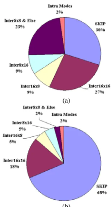
(a)
(b)
Figure 3. Mode distribution. (a) QP = 24. (b) QP = 40.
Figure 4. The current macroblock X and its neighboring macroblocks A, B, C, and D.
1) Analysis
We first observe the relationship between the selected mode and the encoded video content. In general, the SKIP mode or the 16x16 mode is the best mode for macroblocks in the background or the smooth regions of the images. On the other hand, smaller block size, such as the 8x8 mode and the 4x4 mode, are chosen as the best modes on object boundaries, complex textures, and fast moving regions of images.
Using the H.264 reference software JM 8.5, we encoded 8 test sequences (Silent, Tempete, Flower, Container, Foreman,
Mobile, Stefan, and Mother & Daughter) at CIF resolution to
analyze their mode distribution. The result is shown in Figure 3. Based on our analysis, about 30% to 70% of the macroblocks are encoded with the SKIP mode. This important result indicates that the SKIP mode is a good initial guess for fast mode decision.
We analyze the relationship between the mode and the encoded video content. It is observed that when an video object moves, all parts of the video object tend to move together. This implies the existence of temporal and spatial correlations of modes. Now the question is: how the modes of neighboring macroblocks are related to the mode of the current macroblock. The neighboring macroblocks under consideration are shown in Figure 4. With respect to the current macroblock X, macroblocks A, B, C, and D denote the left, top, right-top, and left-top macroblocks of X, respectively. The result of our analysis is shown in Table 1. It is interesting to note that if macroblocks A, B, C, and D have the same mode, it is about 60% to 90% likely that the current macroblock would have the
same mode as well (Case 2). This is a useful piece of information we may use to predict the mode of the current macroblock based on the modes of its neighboring macroblocks.
Intuitively, the probability that three out of the four neighboring macroblocks have the same mode should be higher than the probability that all four neighboring macroblocks have the same mode. However, the likelihood that the current macroblock favors the majority mode would decrease. This is clearly supported by the empirical results shown in Table 1, where Case 3 has a higher percentage than Case 1 but Case 4 gets a lower percentage than Case 2. In this work, we call the mode used in Case 1 and Case 3 as the majority mode.
Table 1. Percentage of similar modes for neighboring macroblocks Sequence QP Case 1 (%) Case 2 (%) Case 3 (%) Case 4 (%) 24 6.3 63.0 30.6 46.7 Foreman 40 36.1 88.2 69.3 74.8 24 11.0 62.0 44.9 52.8 Mobile 40 21.8 78.7 55.4 63.8 24 41.2 95.0 62.2 82.7 Silent 40 66.7 96.3 84.3 90.1 24 6.6 58.8 34.1 46.9 Tempete 40 17.6 75.5 54.0 58.3 24 10.6 61.8 44.8 50.6 Flower 40 16.5 76.2 48.3 57.9 24 22.7 82.6 53.0 65.9 Container 40 78.8 97.3 91.7 93.3 24 10.0 64.5 41.3 49.7 Stefan 40 21.5 84.3 53.0 64.5 24 36.5 92.8 57.7 77.2 Mother & Daughter 40 73.8 95.9 91.3 91.6
Case 1: Macroblocks A, B, C, and D have the same mode.
Case 2: Macroblock X has the same mode as that of macroblocks A, B, C, and D when Case 1 is true.
Case 3: Macroblocks A, B, and D have the same mode.
Case 4: Macroblock X has the same mode as that of macroblocks A, B, and D when Case 3 is true.
Furthermore, we analyze how the modes of neighboring macroblocks correlate with the mode of current macroblock in the case where the majority mode does not exist or is not the best mode. Table 2 shows the percentage of similar modes for neighboring macroblocks in the case. Note that the block size corresponding to the majority mode is excluded from the consideration.
Table 2. Percentage of similar modes Sequence QP Case I (%) Case II (%)
24 72.3 57.6 Foreman 40 41.6 68.8 24 67.4 64.3 Mobile 40 55.8 65.9 24 41.0 59.8 Silent 40 20.0 62.9 24 72.5 60.4 Tempete 40 60.7 66.3 24 68.6 67.3 Flower 40 63.1 63.9 24 55.9 62.4 Container 40 12.1 75.7
24 68.2 63.3 Stefan 40 56.8 66.7 24 46.7 55.0 Mother & Daughter 40 13.0 71.8
Case I: The majority mode does not exist or is not the best mode.
Case II: One of the modes that correspond to the neighboring block of the current block is the same as that of Macroblock X when Case I is true. The results shown in Table 2 indicate that the modes considered in Case I are also useful for mode prediction. We exploit this useful information to predict the possible mode. We call these modes as the secondary modes in our algorithm. The selection method of secondary modes is described below:
• Majority mode exists. The secondary mode is chosen form the modes of the neighboring blocks. Here, the majority mode is excluded from the consideration when determining the secondary mode. Figure 5 (a) shows an example of this case.
• Majority mode does not exist and two out of the four neighboring blocks have the sane mode. Figure 5 (b) and 5 (c) are examples of this case. In Figure 5(b), both M1 and
M2 are chosen as the secondary modes. The smaller block
mode between M1 and M2 is tested first. In Figure 5(c),
only M1 has to be tested.
• A, B, C, and D are in different modes (Figure 5 (d)). In this case, only the largest neighboring block mode of the current block is selected as the secondary mode.
As described above, this step is introduced to examine the secondary mode after the majority mode is tested. Note that the block size of the secondary mode may be larger than the block size of the majority mode.
2) Algorithm Description
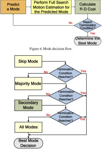
Figures 6-7 show our proposed fast mode decision scheme. The computational load of the mode decision process can be reduced by predicting the best mode and skipping the expensive motion estimation step for all remaining candidate modes.
In our scheme, we predict the current mode based on the previously encoded macroblocks. Therefore, it is important to have a good head start in the chain of predictions. We apply the exhaustive search method for macroblocks that are located in the first row or the first column of the image to ensure that a correct mode is always obtained for such macroblocks.
(a) (b)
(c) (d) Figure 5. Examples of the secondary mode.
Figure 6. Mode decision flow.
Figure 7. Mode prediction flow.
In the mode decision process, we need to measure the goodness of a prediction. Two different thresholds TSKIP and T1
are used, the first one for SKIP mode prediction and the second one for mode similarity test. Since a fixed threshold may not work well, the values of TSKIP and T1 are determined adaptively.
TSKIPis an adaptive threshold determined by the average R-D
cost of all coded macroblocks of the skip mode. T1 is the
average R-D cost of the macroblocks of the majority mode or the secondary mode. Moreover, a weighting factor α is introduced to control the speed and the coding quality in our algorithm (α = 0.8 in our simulations).
The proposed fast mode decision algorithm consists of the following steps:
Step 1: If the current macroblock is located in the first column or the first row of the image, examine all available modes. Calculate the R-D costs of all available modes, select the best one, and stop.
Step 2: Examine the skip mode and calculate its R-D cost. If this cost is smaller than α*TSKIP, set the skip mode as the
best mode and stop.
Step 3: Check the availability of macroblocks A, B, C, and D. If all of them are available, go to Step 4. Otherwise, go to Step 5.
Step 4: If more than two neighboring macroblocks A, B, C, and D have the same mode, go to Step 6. Otherwise, go to Step 5.
Step 5: If more than one neighboring macroblocks A, B, and D have the same mode go to Step 6. Otherwise, go to Step 7.
Step 6: Calculate the R-D cost of the majority mode. If this cost is smaller than T1, choose the majority mode as the
best mode and stop. Otherwise, go to Step 7.
Step 7: Examine the secondary mode and calculate its R-D cost. If this cost is smaller than T1, choose the secondary
mode as the best mode and stop. Otherwise, go to Step 8.
Step 8: Examine the remaining modes and calculate their R-D costs. Select the best one and stop.
Note that J(mode) stands for the rate-distortion cost of
mode. Step 8 is applied when no best mode has been chosen at
the end of Step 7.
In our proposed fast mode decision scheme, even though ME does not need to be performed for some block types, it still involves a lot of computation at the encoder. Therefore, we propose a fast multi-frame motion estimation algorithm for reducing the computational complexity in the next section.
B. Fast Motion Estimation
In this section, we present a fast multi-frame motion estimation algorithm. This algorithm is based on an adaptive search strategy and a flexible multi-frame search scheme.
In general, the matching process in our fast ME visits the seven block sizes [1], from 16x16 to 4x4, in a hierarchical descending order. Like wise, in the case of multiple reference frames, the references frames are visited sequentially starting from the previous frame for each macroblock to be coded. However, the modes to be visited in the combined fast motion estimation and mode decision algorithm may not follow the descending order due to the introduction of the FMD algorithm. More specifically, the mode prediction procedure in the FMD algorithm is based on the modes of the neighboring macroblocks, not the order of block sizes.
1) Adaptive Search Strategy
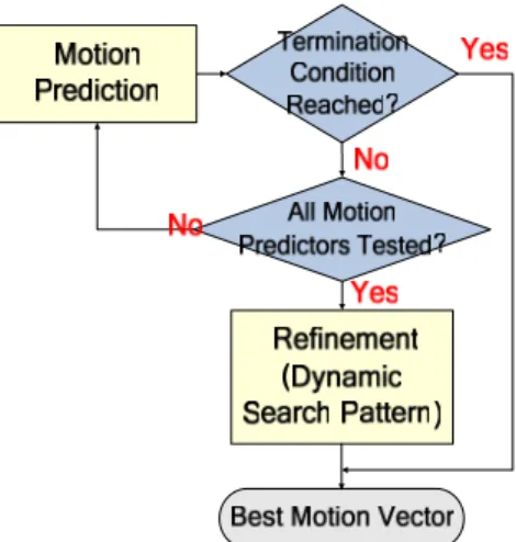
Figure 8 illustrates the flow of adaptive search strategy for a testing mode. To increase the hit rate, five motion predictors are employed in our motion estimation algorithm, which sequentially tests the five predictors and stops when an early termination condition described below is reached or when all five predictors are tested. When no early termination is detected at the end, a dynamic search pattern is applied to refine the motion vector.
A) Motion prediction
Five motion predictors are used to find the best initial search point in the motion estimation process, by exploiting the temporal and spatial correlations of motion vectors in a video sequence. To increase the hit rate, five motion predictors are employed in our motion estimation algorithm. The average hit rate of five combined motion predictors achieves 69%.
Figure 8. Flowchart for adaptive search strategy.
These five predictors are tested sequentially according to the order: median predictor, upper-layer predictor, spatial predictor, temporal predictor, and accelerator predictor. The process stops when an early termination condition described below is reached or when all five predictors are tested. When no early termination is detected at the end, a dynamic search pattern is applied to refine the motion vector. Note that the motion vectors referred to in this section are obtained with respect to the reference frame under consideration.
a) Median predictor:The median value of motion vectors of adjacent blocks on the left, top, and top-right of the current block is used to predict the motion vector of the current block to be coded.
pred -median left top top-right
V = median (V , V , V ), (29)
where Vleft, Vtop, and Vtop-right are motion vectors of the left, top,
and top-right blocks, respectively. The median operation is performed on each component of the motion vector.
b) Neighboring-layer predictor: The different modes tested in one macroblock are considered as different layers [24], [25]. With respect to the layer under consideration, the lower layer is considered as smaller block modes than the testing mode, and the upper layer is considered as larger block modes. For example, the 16x16 mode is the upper layer of the 16x8 and 8x16 modes; the 8x8, 8x4, 4x8, and 4x4 modes are regarded as the lower layers of those. The motion vectors of the neighboring-layer (upper-layer and lower-layer) block are used as the motion predictor for the current block mode.
Figure 9 illustrate the example of neighboring-layer predictor. In Figure 9 (a), the motion vector of partition 0 of mode 2 can be used as the motion prediction for partitions 0 and 1 of mode 4. With respect to the layer under consideration, the lower-layer predictor is selected as the motion predictor if both upper-layer and lower-layer blocks have been examined. This motion predictor is used because the motion vectors of smaller blocks are expected to have better prediction of the motion behavior in a macroblock.
c) Spatial predictor: The motion vectors of adjacent blocks (left, top, and top-right) that have the same mode as the
current block are used as the motion predictor of the current block.
d) Temporal predictor: The motion vectors of corresponding blocks in the neighboring frames are used as the motion predictors of the current block.
e) Accelerator predictor: For high motion sequences, the object may move with increasing or decreasing acceleration [19]. To deal with such cases, an accelerator predictor is used and defined as follows:
1 1 2
pred -accel t - t - t
-V = V + (V -V ) , (30) where Vt-1 is the motion vector of corresponding block in the
previous frame t–1, and Vt-2 is the motion vector of
corresponding block in frame t–2. Figure 10 shows an example of accelerator predictor.
When no early termination condition is reached, the motion predictor with the smallest Lagrangian cost [1] is chosen as the best motion prediction Pbest.
B) Adaptive early termination
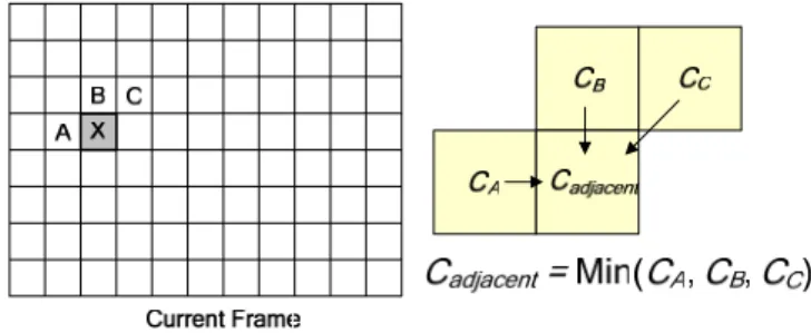
An early termination of motion prediction and refinement is applied when the video quality is good enough. By exploiting the correlations [14], [15] of Lagrangian costs, a threshold to determine the video quality of the current block is derived based on the Lagrangian costs of its neighboring blocks with respect to the reference frame under consideration. Here, we set this threshold Cpred to be the smallest value among Cadjacent,
Clayer, and Cref defined in the following.
(a)
(b)
Figure 9. Illustration of neighboring-layer predictor.
Figure 10. Example of accelerator predictor.
a) Cadjacent: The smallest Lagrangian cost of the adjacent
blocks (left, top, and top-right) that have the same mode as the current block, as shown in Figure 11. X is the current block.
CA, CB, and CC denote the smallest Lagrangian costs of the left,
top, and top-right blocks, respectively.
b) Clayer: A value derived from the smallest Lagrangian
cost of the neighboring layers. Similar to the neighboring-layer motion predictor, the smallest Lagrangian cost of lower-layer block is used to derive the termination threshold Clayer if both
the upper-layer and lower-layer blocks have been examined. If the value Clayer derived from the upper layer, Clayer is computed
by Equation 31. Otherwise, Clayer is computed by Equation 32.
2 0 9 layer upper -layer
C = (C / )⋅ . . (31)
0 0 1 1 2 3
layer , layer ,
C = (C + C , C) = (C + C ). (32) Because smaller blocks are expected to have a better prediction, a multiplication factor 0.9 is applied in the equation.
c) Cref: A termination threshold of Lagrangian cost for
the reference block in frame t’ (the reference frame under consideration). If there is no uncovered background or occluded object in a macroblock, the difference of Lagrangian costs of a block between different reference frames is small. Based on this property, Cref is computed by
1
ref t'
C = C + , (33) where Ct’+1 is the Lagrangian cost of the same block in frame t’
+1 (t’
< t–1), as shown in Figure 13. When t’=t – 1, Cref is set to
a very large number.
In order to avoid using an extremely large threshold (and thereby ensure the video quality), Cpred is limited to 3*Ti (Ti is
computed by Equation 35). The matching process for the current block is terminated when the Lagrangian cost (Ccurr) of
the current block is smaller than Cpred.
Figure 11. Illustration of early termination threshold Cadjacent.
(a) (b) Figure 12. Examples of early termination threshold Clayer.
Figure 13. Example of early termination threshold Cref.
C) Dynamic search pattern
This scheme is applied for motion refinement. We set the search center at the position pointed to by Pbest. The mechanism
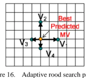
of the dynamic search pattern selection is shown in Figure 14. The refinement search pattern is selected from four candidates: large cross search pattern (Figure 15 (a)), hexagon search pattern (Figure 15 (b)), cross search pattern (Figure 15 (c)), and adaptive rood search pattern (Figure 16). When Δ =CC curr –
Cpred is smaller than the threshold H2, the best motion vector is
expected to be close to Pbest. In this case, the cross search
pattern is used to refine the motion vector. Else if Δ ≦ HC 1,
the hexagon search pattern is used to refine the motion vector. If Δ > HC 1, the refinement search pattern is selected between
the rood search pattern and the large cross search pattern based on the magnitude of Vpred-median (we set the threshold Vth to 7).
For low and medium motion sequences, the rood search pattern often obtains the best motion vector accurately and rapidly. However, it does not perform well for high motion sequences. Therefore, the large cross search pattern is adopted to refine the motion vector for high motion sequences.
Figure 14. The flowchart of the dynamic search pattern selection.
Figure 15. (a) Large cross search pattern. (b) Hexagon search pattern. (c) Cross search pattern.
Figure 16. Adaptive rood search pattern.
2) Flexible Multi-Frame Search Scheme
With multiple reference frames, the computational cost can increase significantly [26]. We develop a flexible multi-frame search scheme that avoids unnecessary search operations.
A matching is good if the quantized transform coefficients of the motion-compensated block are all close to zeros. A block with all zero quantized transform coefficients is called as a zero block [25]. A threshold is used in our algorithm. When the SAD of a motion-compensated block is smaller than the threshold, this block is considered a zero block. When the SAD of a motion-compensated block is smaller than the threshold, this block is considered as a zero block. When a zero block is detected, the remaining modes and reference frames are skipped and not searched. The threshold T7 is derived based on
4x4 blocks [25]:
7 2 0 0
qbits
const coeff rem
T = ( - qp ) / Q [q ][ ][ ]
.
(34) where qbits=15 + QP/6, qpconst = (1<<qbits)/6, qrem= (QP mod6), Qcoeff is the quantization coefficient table, and QP is the
quantization parameter.
For the other modes of block sizes 16x16, 16x8, 8x16, 8x8, 8x4, and 4x8, the threshold is defined as:
Ti = T7 x mi, (35)
where mi is a scale factor (in our experiment, mi = 4, 2.5, 2.5, 2,
1.5, 1.5, for i = 1…6). Like the mechanism used in early termination, a cap is applied to the threshold. The cap is set to 512, 448, 448, 384, 384, 384, and 384, respectively, for i = 1...7.
This termination condition is examined after the ME for each mode is performed. A flag Tflag is set to 1 when this
termination condition for the modes and the reference frames is reached. In case of Tflag = 1, the remaining modes and reference
frames are skipped without computing and comparing the R-D costs.
When a zero block is detected, the Intra 4x4 prediction mode will be skipped. This is because, in practice, the Intra 4x4
prediction mode is rarely selected as the best mode in such cases.
Figure 17. The flow of combined algorithm.
Figure 18. Interaction between the FME and FMD modules
3) Architecture of Combined Algorithm
As described before, we presented a fast mode decision and fast multi-frame motion estimation algorithms. For our combined algorithm, we allows the FMD to interact with FME to reduce the computational cost while maintaining picture quality and coding efficiency, as shown in Figures 17-18.
The FMD module in the combined algorithm predicts the mode of the current block. This mode information is input to the FME module, where the motion search is performed. After the motion search for the predicted mode Mpred is done, the
FME module sends the motion vector VMpred and Tflag to the
FMD module. The FMD module decides whether it should search other modes or not based on an adaptive threshold and the flag Tflag obtained from the FME module.
V. SIMULATION RESULTS
A. Transcoding and Downsampling
The performance comparison between two different transcoding architectures is presented. One is the full-decompression and full compression architecture (referred to as the cascade architecture), and the other is our proposed architecture. In the experiment, the DCT-to-PEL transcoding architecture is adopted for I-frames, since intra prediction in the spatial domain is much easier to implement.
In the experiment the input is a CIF sequence and the output is a QCIF sequence, with frame rate equal to 30 fps. The GOP size (N) used is 15 and the picture sub-group size (M, distance between I and P frames) is 1. The bit rate of the MPEG-2 bitstream is 4 Mbit/s.
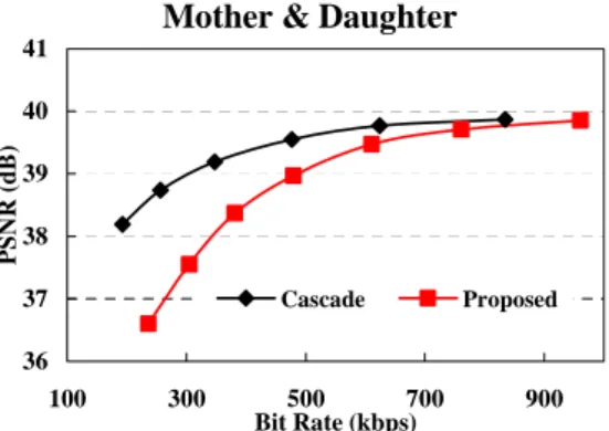
The performance comparisons for Foreman and Mother &
Daughter sequence are shown in Figures 19-20. It can be seen
that the proposed architecture can achieve quality comparable
to the full decoding and full encoding architecture when target bit rate is about 900 kbps.
Foreman
30 31 32 33 34 200 400 600 800 1000 Bit Rate (kbps) PSNR ( d B) Cascade ProposedFigure 19. Performance comparison for Foreman sequence.
Mother & Daughter
36 37 38 39 40 41 100 300 500 700 900 Bit Rate (kbps) PSNR ( d B) Cascade Proposed
Figure 20. Performance comparison for Mother & Daughter sequence.
B. Optimization of H.264
Our proposed algorithms were implemented in the H.264 reference software JM 8.5. In our simulation, the search range of motion vector was set to
±
32 pels for CIF resolution. Apart from the first frame, all the other frames were coded as P frames. Furthermore, R-D optimization, CAVLC entropy coding, and seven block modes were turned on for all tests. The simulation conditions used in H.264 reference software are shown in Table 3. The simulations were performed on a PC with a Pentium IV, 2.4 GHz CPU, and a 768 MB RAM.We used various sequences to evaluate the performance of the proposed algorithms. To simplify our comparisons, we used Bjontegaard delta PSNR (BDPSNR) and Bjontegaard delta bit rate (BDBR) [45].
Table 3. Simulation conditions
Frame Rate 30 fps
Hadamard Transform Used
Image Size 352x288
Search Range 32
Sequence Type IPPP
Entropy Coding Method CAVLC RD-Optimized Mode Decision Used
QP 28, 32, 36, 40
1) Fast Mode Decision
Our algorithm achieves an average of 2.21 times speedup in total encoding time when one reference frame is used and 2.11 times speedup when five reference frames are used.
Table 4. PSNR Comparison (1 reference frame) Sequence (CIF) BDPSNR (dB) BDBR ME Speedup Encoding Speedup M & D -0.088 1.35% 2.35 2.44 Container -0.203 3.21% 2.67 2.73 Silent -0.118 1.87% 2.07 2.21 Foreman -0.169 2.63% 1.70 1.84 Stefan -0.193 2.35% 1.63 1.83 Average -0.154 2.28% 2.08 2.21
Table 5. PSNR Comparison (5 reference frames) Sequence (CIF) BDPSNR (dB) BDBR ME Speedup Encoding Speedup M & D -0.079 1.18% 2.32 2.33 Container -0.146 2.20% 2.52 2.71 Silent -0.100 1.66% 2.05 2.09 Foreman -0.142 2.14% 1.68 1.72 Stefan -0.177 2.21% 1.64 1.70 Average -0.129 1.87% 2.04 2.11
Table 6. Comparison of average PSNR Number of Ref. Frames BDPSNR (dB) BDBR ME Speedup Encoding Speedup 1 Frame -0.154 2.28% 2.08 2.21 5 Frames -0.129 1.87% 2.04 2.11
2) Fast Multi-Frame Motion Estimation
Tables 7-8 show the performance comparison of our algorithm against UMHexagonS and the fast full search used in JM 8.5. On the average, our algorithm is 55.6 faster than the fast full search and 3.5 times faster than UMHexagonS, with negligible bit rate increase and PSNR drop.
Table 7. PSNR Comparison (1 reference frame) Sequence (CIF) Search Method BDPSNR (dB) BDBR ME Speedup Encoding Speedup UMHexagonS -0.024 0.27% 9.75 1.92 Mobile FME -0.039 0.44% 37.31 2.17 UMHexagonS -0.031 0.40% 10.61 2.04 Tempete FME -0.087 1.10% 37.21 2.36 UMHexagonS -0.019 0.20% 10.74 1.90 Flower FME -0.042 0.44% 36.59 2.18 UMHexagonS -0.034 0.50% 21.34 2.50 M & D FME -0.056 0.84% 50.71 3.14 UMHexagonS -0.064 0.95% 19.13 2.34 Container FME -0.100 1.49% 47.78 2.59 UMHexagonS -0.025 0.42% 16.17 2.30 Silent FME -0.080 1.27% 42.74 2.57 UMHexagonS -0.057 0.88% 12.61 2.26 Foreman FME -0.167 2.63% 38.32 2.59 UMHexagonS -0.038 0.45% 11.46 2.07 Stefan FME -0.107 1.30% 36.84 2.41 UMHexagonS -0.035 0.50% 14.22 2.18 Average FME -0.085 1.19% 40.94 2.50
Table 8. PSNR Comparison (5 reference frames) Sequence (CIF) Search Method BDPSNR (dB) BDBR ME Speedup Encoding Speedup UMHexagonS -0.014 0.16% 10.85 3.66 Mobile FME -0.037 0.43% 44.98 4.88 UMHexagonS -0.018 0.24% 11.81 3.92 Tempete FME -0.046 0.59% 47.28 5.43 UMHexagonS -0.019 0.21% 11.14 3.62 Flower FME -0.038 0.42% 44.57 4.99 UMHexagonS -0.027 0.43% 22.89 5.29 M & D FME -0.045 0.71% 86.33 8.18 UMHexagonS -0.044 0.68% 23.13 5.06 Container FME -0.073 1.14% 68.08 6.51 UMHexagonS -0.031 0.50% 19.02 4.76 Silent FME -0.069 1.13% 57.78 6.13 UMHexagonS -0.050 0.75% 13.15 4.37 Foreman FME -0.152 2.28% 51.52 6.31 UMHexagonS -0.019 0.24% 11.02 3.87 Stefan FME -0.092 1.14% 44.73 5.60 UMHexagonS -0.028 0.41% 15.78 4.37 Average FME -0.069 0.98% 55.65 6.00
Table 9. Comparison of average PSNR Number of Ref. Frames Search Method BDPSNR (dB) BDBR ME Speedup Encoding Speedup UMHexagonS -0.035 0.50% 14.22 2.18 1 Frame FME -0.085 1.19% 40.94 2.50 UMHexagonS -0.028 0.41% 15.78 4.37 5 Frames FME -0.069 0.98% 55.65 6.00 3) Combined Algorithm
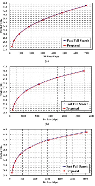
Our algorithm is compared with the fast full search used in JM 8.5. Tables 10-11 show the results of performance comparison for one and five reference frames. On the average, our algorithm is 12 times faster than the fast full search in the total encoding time. Figure 21 shows the R-D performance comparison between our algorithm and fast full search for various test images at CIF resolution. On the average, the performance degradation of our algorithm is less than 0.3 dB and the bit rate increase is less than 4.5%.
Table 10. PSNR Comparison (1 reference frame) Sequence (CIF) BDPSNR (dB) BDBR Encoding Speedup Mobile -0.164 1.83% 5.80 Tempete -0.215 2.73% 6.22 Flower -0.150 1.64% 6.06 M & D -0.117 1.81% 8.38 Container -0.180 2.71% 8.26 Silent -0.176 2.79% 7.04 Foreman -0.271 4.30% 6.51 Stefan -0.280 3.44% 6.72 Average -0.194 2.66% 6.87
Table 11. PSNR Comparison (5 reference frames) Sequence (CIF) BDPSNR (dB) BDBR Encoding Speedup Mobile -0.172 2.03% 9.88 Tempete -0.178 2.28% 10.64 Flower -0.147 1.63% 10.15 M & D -0.087 1.33% 16.03 Container -0.162 2.44% 15.31 Silent -0.158 2.43% 12.37 Foreman -0.235 3.56% 11.74 Stefan -0.241 3.04% 11.27 Average -0.172 2.35% 12.17
Table 12. Comparison of average PSNR Number of Ref. Frames BDPSNR (dB) BDBR Encoding Speedup 1 Frame -0.194 2.66% 6.87 5 Frames -0.172 2.35% 12.17
22.0 24.0 26.0 28.0 30.0 32.0 34.0 36.0 38.0 40.0 42.0 44.0 46.0 0 1000 2000 3000 4000 5000 6000 7000 Bit Rate (kbps) P S NR-Y ( d B )
Fast Full Search Proposed (a) 25.0 27.0 29.0 31.0 33.0 35.0 37.0 39.0 41.0 43.0 45.0 47.0 0 1000 2000 3000 4000 5000 6000 Bit Rate (kbps) P S NR-Y (d B )
Fast Full Search Proposed (b) 28.0 30.0 32.0 34.0 36.0 38.0 40.0 42.0 44.0 46.0 0 500 1000 1500 2000 2500 3000 Bit Rate (kbps) PS NR-Y (d B)
Fast Full Search Proposed
(c)
Figure 21. R-D performance comparison for (a) Flower, (b) Stefan, and (c)
Foreman sequences using 5 reference frames.
VI. ACHIEVEMENTS
A. Publications
[1] C. Chen, P.-H. Wu, and H. H. Chen, “Transform-Domain intra prediction for H.264,” in Proc. IEEE Int.
Symposium on Circuits and Systems, pp. 1497-1500,
May 2005.
[2] C. Chen, B.-H. Wu, and H. H. Chen, “Rounding in the transform domain for multimedia systems,” International
Conference on Wireless Networks, Communications, and Mobile Computing, Maui, Hawaii, Jun. 2005.
[3] C. Chen, B.-H. Wu, and H. H. Chen, “A practical solution to transform-domain rounding,” 13th European
Signal Processing Conference, Sept. 2005.
[4] C.-Y. Chang, C.-H. Pan, and H. H. Chen, “Fast mode decision for P-frames in H.264,” Picture Coding
Symposium, Dec. 2004.
[5] S.-F. Lin, M.-T. Lu, C.-H. Pan, and H. H. Chen, “Fast
multi-frame motion estimation for H.264 and its applications to complexity-aware streaming,” in Proc.
IEEE Int. Symposium on Circuits and System, pp.
1505-1508, May 2005.
[6] S.-F. Lin, C.-Y. Chang, C.-C. Su, Y.-L. Lin, C.-H. Pan, and H. H. Chen, “Fast multi-frame motion estimation and mode decision for H.264 encoders,” International Conf.
on Wireless Networks, Communications, and Mobile Computing, Maui, Hawaii, Jun. 2005.
B. Patents
[1] 視訊編碼裡加速模式判定的方法,中華民國專利申請 中,申請案號:93139134,發明人:陳宏銘、張哲瑜、 潘佳河.
[2] Method to Speed up the Mode Decision of Video Coding, US patent pending, inventor: H. H. Chen, C.-Y. Chang, and C.-H. Pan.
REFERENCES
[1] “Draft ITU-T recommendation and final draft international standard of joint video specification (ITU-T Rec. H.264/ISO/IEC 14496-10 AVC),” in Joint Video Team (JVT) of ISO/IEC MPEG and ITU-T VCEG, JVT-G050, 2003.
[2] N. Merhav and V. Bhaskaran, “Fast algorithm for DCT-domain image down-sampling and for inverse motion compensation,” IEEE Trans. Circuits Syst. Video
Technol., vol. 7, pp. 468 -476, Jun. 1997.
[3] C. Chen, P.-H. Wu, and H. Chen, “Transform-Domain intra prediction for H.264,” in Proc. IEEE Int.
Symposium on Circuits and Systems, pp. 1497-1500,
May 2005.
[4] S.-F. Chang and D. G. Messerschmitt, “Manipulation and compositing of MC-DCT compressed video,” IEEE J.
Select. Areas Commun., vol. 13, pp. 1-11, Jan. 1995.
[5] P. A. A. Assuncao and M. Ghanbari, “Transcoding of MPEG-2 video in the frequency domain,” in Proc. IEEE
Int. Conf. Acoustics., Speech, Signal Processing, ICASSP’97, vol. 4, pp. 2633-2636, Apr. 1997.
[6] J. Song and B.-L. Yeo, “A fast algorithm for DCT-domain inverse motion compensation based on shared information in a macroblock,” IEEE Trans.
Circuits Syst. Video Technol., vol. 10, pp. 767-775, Aug.
2000.
[7] T. Shanableh and M. Ghanbari, “Hybrid DCT/pixel domain architecture for heterogeneous video transcoding,” Signal Processing: Image Commun., vol. 18, no. 8, pp. 601-620, Sep. 2003.
[8] P. Yin, A. Vetro, B. Liu, and H. Sun, “Drift compensation for reduced spatial resolution transcoding,” IEEE Trans. Circuits Syst. Video Technol., vol. 12, pp. 1009-1020, Nov. 2002.
[9] T. Shanableh and M. Ghanbari, “Heterogeneous video transcoding to lower spatial-temporal resolutions and different encoding formats,” IEEE Trans. Multimedia, vol. 2, Jun. 2000.
[10] http://bs.hhi.de/~suehring/tml/download/, JVT reference software.
[11] A. Vetro, C. Christopoulos, and H. Sun, “Video transcoding architectures and techniques: An overview,”
IEEE Signal Processing Magazine, pp. 18-29, Mar.
2003.
[12] J. Xin, C.-W. Lin, and M.-T. Sun, “Digital video transcoding,” in Proc. IEEE, vol. 93, no. 1, pp. 84-97, Jan. 2005
[13] ISO/IEC 13818-2, “Information technology–Generic coding of moving pictures and associated audio information: Video,” 1995.
[14] G. J. Sullivan and T. Wiegand, “Rate-distortion optimization for video compression,” IEEE Signal
Processing Magazine, pp. 74-90, Nov. 1998.
[15] A. Joch, F. Kossentini, H. Schwarz, T. Wiegand, and G. Sullivan, “Performance comparison of video coding standards using Lagrangian coder control,” in Proc.
IEEE Int. Conf. on Image Processing, pp. 501–504, Sept.
2002.
[16] S. Zhu and K. K. Ma, “A new diamond search algorithm for fast block-matching motion estimation,” IEEE Trans.
Image Processing, vol. 9, pp. 287-290, Feb. 2000.
[17] C. Zhu, X. Lin, and L.-P. Chau, “Hexagon-based search pattern for fast block motion estimation,” IEEE Trans.
Circuits Syst. Video Technol., vol. 12, no. 5, pp. 349-355,
May 2002.
[18] P. I. Hosur and K. K. Ma, “Motion vector field adaptive fast motion estimation,” Proc. 2nd Int. Conf. Information,
Communications and Signal Processing, Dec. 1999.
[19] H.-Y, C. Tourapis, A. M. Tourapis, and P. Topiwala, “Fast motion estimation within the JVT codec,” JVT-E023.doc, Joint Video Team (JVT) of ISO/IEC MPEG & ITU-T VCEG, 5th meeting, Oct. 2002.
[20] K. K. Ma and G. Qiu, “Unequal-arm adaptive rood pattern search for fast block-matching motion estimation in the JVT/H.26L,” in Proc. IEEE Int. Conf. on Image
Processing, Sept. 2003.
[21] A. M. Tourapis, O. C. Au, and M. L. Liou, “Predictive motion vector field adaptive search technique (PMVFAST)- enhancing block based motion estimation,” in Proc. Visual Communications and Image
Processing, pp. 883-892, Jan. 2001.
[22] A. M. Tourapis, O. C. Au, and M. L. Liou, “New results on zonal based motion estimation algorithms- advanced predictive diamond zonal search,” in Proc. IEEE Int.
Symposium on Circuits and Systems, vol.5, pp.183-186,
May 2001.
[23] A. M. Tourapis, O. C. Au, and M. L. Liou, “Highly efficient predictive zonal algorithms for fast block-matching motion estimation,” IEEE Trans.
Circuits Syst. Video Technol., vol. 12, pp. 934–947, Oct.
2002.
[24] Z. Chen, P. Zhou, and Y. He, “Fast integer pel and fractional pel motion estimation for JVT,” JVT-F017r1.doc, Joint Video Team (JVT) of ISO/IEC MPEG & ITU-T VCEG, 6th meeting, Dec. 2002. [25] Z. Chen, P. Zhou, and Y. He, “Fast motion estimation for
JVT,” JVT-G016.doc, Joint Video Team (JVT) of ISO/IEC MPEG & ITU-T VCEG, 7th Meeting, Mar.
2003.
[26] Y.-W. Huang, et al., “Analysis and reduction of reference frames for motion estimation in MPEG-4 AVC/JVT/H.264,” in Proc. IEEE Int. Conf. on Acoustics,
Speech, and Signal Processing, Apr. 2003.
[27] I-M. Pao and M.-T. Sun, “Modeling DCT coefficients for fast video encoding,” IEEE Trans. Circuits Syst. Video
Technol., vol. 9, no. 4, pp. 608-616, Jun. 1999.
[28] P. Yin, H.-Y. Tourapis, A. M. Tourapis, and J. Boyce, “Fast mode decision and motion estimation for H.264,” in Proc. IEEE Int. Conf. on Image Processing, vol. III, pp. 853-856, Sept. 2003.
[29] D. Wu, S. Wu, K. P. Lim, F. Pan, and X. Lin, “Block inter mode decision for fast encoding of H.264,” in Proc.
IEEE Int. Conf. on Speech, Acoustics, and Signal Processing, vol. 3, pp. 181-184, May 2004.
[30] F. Pan, X. Lin, S. Rahardja, K. P. Lim, and Z. G. Li, “A directional field based fast intra mode decision algorithm,” in Proc. IEEE Int. Conf. on Multimedia and
Expo 2004, Jun. 2004.
[31] C. Blanch and K. Denolf, “Memory complexity analysis of the AVC codec JM 1.7,” ISO/IEC JTC1/WG11 MPEG02/M8378 Fairfax, May 2002.
[32] W. I. Choi, J. Lee, S. Yang, and B. Jeon, “Fast motion estimation and mode decision with variable motion block sizes,” in Proc. SPIE Visual Communications and Image
Processing, vol. 5150, pp. 1561-1572, 2003.
[33] B. Meng and O. C. Au, “Fast intra-prediction mode selection for 4x4 blocks in H.264,” in Proc. IEEE Int.
Conf. on Acoustics, Speech, and Signal Processing, vol.
3, pp. 389-392, Apr. 2003.
[34] A. Ahmad, N. Khan, S. Masud, and M. A. Maud, “Selection of variable block sizes in H.264,” in Proc.
IEEE Int. Conf. on Acoustics, Speech, and Signal Processing, vol. 3, pp. 173-176, May 2004.
[35] D. S. Turaga and T. Chen, “Estimation and mode decision for spatially correlated motion sequences,”
IEEE Trans. Circuits Syst. Video Technol., vol. 11, no. 10,
pp. 1098-1107, Oct. 2001.
[36] A. C. Yu, “Efficient block-size selection algorithm for inter-frame coding in H.264/MPEG-4 AVC,” in Proc.
IEEE Int. Conf. on Acoustics, Speech, and Signal Processing, vol. 3, pp. 169-172, May 2004.
[37] L. P. Kondi, “A rate-distortion optimal hybrid scalable/multiple-distortion video codec,” in Proc. IEEE
Int. Conf. on Acoustics, Speech, and Signal Processing,
vol. 3, pp. 269-272, May 2004.
[38] X. Li, J. R. Jackson, A. K. Katsaggelos, and R. M. Mersereau, “An adaptive coding scheme using affine motion model for MPEG P-VOP,” in Proc. IEEE Int.
Conf. on Acoustics, Speech, and Signal Processing, vol.
3, pp. 717-720, May 2004.
[39] Y. J. Liang and K. El-Maleh, “Low-complexity intra/inter mode-decision for H.264/AVC video coder,” in Proc. IEEE Int. Symposium on Intelligent Multimedia,
Video and Speech Processing, pp 53-56, Oct. 2004.
[40] J. Chen, Y. Qu, and Y. He, “A fast mode decision algorithm in H.264,” Picture Coding Symposium, Dec. 2004.
[41] Y. Su and M.-T. Sun, “Fast multiple reference frame motion estimation for H.264,” in Proc. IEEE Int. Conf.
on Multimedia and Expo 2004, vol. 1, pp. 695-698, Jun.
2004.
[42] C.-Y. Chang, C.-H. Pan, and H. H. Chen, “Fast mode decision for P-frames in H.264,” Picture Coding
Symposium, Dec. 2004.
[43] S.-F. Lin, M.-T. Lu, C.-H. Pan, and H. H. Chen, “Fast multi-frame motion estimation for H.264 and its applications to complexity-aware streaming,” in Proc.
IEEE Int. Symposium on Circuits and System, pp.
1505-1508, May 2005.
[44] S.-F. Lin, C.-Y. Chang, C.-C. Su, Y.-L. Lin, C.-H. Pan, and H. H. Chen, “Fast multi-frame motion estimation and mode decision for H.264 encoders,” International Conf.
on Wireless Networks, Communications, and Mobile Computing, Maui, Hawaii, Jun. 2005.
[45] G. Bjontegaard, "Calculation of average PSNR differences between RD-curves," Doc. VCEG-M33, Apr. 2001.
[46] G. Sullivan, "Recommended simulation common conditions for H.26L coding efficiency experiments on low-resolution progressive-scan source material", Doc. VCEG-N81, Sep. 2001.