Combining the cost of reducing uncertainty with the selection of risk
assessment models for remediation decision of site contamination
Yen-Chuan Chen, Hwong-Wen Ma
∗Graduate Institute of Environmental Engineering, National Taiwan University, 71 Chou-Shan Road, Taipei 106, Taiwan
Received 28 December 2005; received in revised form 15 May 2006; accepted 21 June 2006 Available online 30 June 2006
Abstract
The decision as to whether a contaminated site poses a threat to human health and should be cleaned up relies increasingly upon the use of risk assessment models. However, the more sophisticated risk assessment models become, the greater the concern with the uncertainty in, and thus the credibility of, risk assessment. In particular, when there are several equally plausible models, decision makers are confused by model uncertainty and perplexed as to which model should be chosen for making decisions objectively. When the correctness of different models is not easily judged after objective analysis has been conducted, the cost incurred during the processes of risk assessment has to be considered in order to make an efficient decision. In order to support an efficient and objective remediation decision, this study develops a methodology to cost the least required reduction of uncertainty and to use the cost measure in the selection of candidate models. The focus is on identifying the efforts involved in reducing the input uncertainty to the point at which the uncertainty would not hinder the decision in each equally plausible model. First, this methodology combines a nested Monte Carlo simulation, rank correlation coefficients, and explicit decision criteria to identify key uncertain inputs that would influence the decision in order to reduce input uncertainty. This methodology then calculates the cost of required reduction of input uncertainty in each model by convergence ratio, which measures the needed convergence level of each key input’s spread. Finally, the most appropriate model can be selected based on the convergence ratio and cost. A case of a contaminated site is used to demonstrate the methodology.
© 2006 Elsevier B.V. All rights reserved.
Keywords: Multimedia risk assessment model; Model uncertainty; Nested Monte Carlo simulation; Sensitivity analysis
1. Introduction
When a contaminated site is identified, one issue that greatly concerns the public is whether the contamination poses a threat to human health and the environment. The problem then con-fronting decision makers is whether the site should be subject to control or remediation. Since the paradigm of risk assessment and management was established in 1983[1], risk assessment has become an important tool used to assess how human health is impacted by contaminants released from a human activity, transferred through environmental media, and finally exposed to humans via inhalation, ingestion, and dermal contact. Because of its capability of systematically providing information relating risk sources to risk receptors, the results as well as the processes of risk assessment are increasingly used to facilitate decisions
∗Corresponding author. Tel.: +886 2 2363 0406; fax: +886 2 2392 8830.
E-mail address:hwma@ntu.edu.tw(H.-W. Ma).
regarding whether a contaminated site should be remediated and what degree of remediation is needed [2,3]. In practice, risk assessment involves modeling of multimedia transport and multiple pathway exposure and requires detailed site-specific information to enable accurate simulation of the situation. This information includes source conditions, land use properties, res-ident lifestyles, and environmental characteristics as well as the inherent individual, spatial, and temporal variability of the above information. However, the more sophisticated risk assessment models become, through inclusion of such concepts as stochas-ticity, multimedia transfer, and site-specificity, the greater the concern with the uncertainty in, and thus the credibility of, risk assessment. In particular, when there are several equally plausi-ble models, it is difficult to select one for the purpose of facilitat-ing decision-makfacilitat-ing. The issue of model selection results from model uncertainty and constitutes a part of model uncertainty.
The purpose of using models is to clarify the problem and facilitate decision-making. However, uncertainty in the use of models may confuse the decision-making process. To resolve 0304-3894/$ – see front matter © 2006 Elsevier B.V. All rights reserved.
the confusion, it may be necessary to question how a model can support the decision. For a model to be helpful, the asso-ciated uncertainty should not be too large. The purpose of this study is to develop a methodology to measure the least required reduction of uncertainty and to use the measure in the selection of candidate models. A decision problem about a contaminated site is used as a case study to demonstrate the methodology.
The rest of the paper is organized as follows. Section2 sum-marizes the uncertainty in risk assessment modeling approaches. Section3outlines the methodology, and Section4presents the results and discussion associated with the decision problem. Finally, the concluding remarks are provided in Section5.
2. Uncertainty in risk assessment modeling
This study explores how to choose among equally plausible models for risk-related decisions. The issue of model selection is closely related to model uncertainty, which is described in this section along with brief descriptions of other types of uncer-tainty.
Many classifications of sources of uncertainty in risk assess-ment are discussed in the literature[4–8]. Three representative classifications are listed inTable 1. Although some of the tax-onomies are the same, they are not clearly separated. The same definitions in different classifications comprise variability (also called stochastic, aleatory, or Type A uncertainty[4,7,8]) and input uncertainty (also called subjective, epistemic, or Type B uncertainty [4,7,8]). Variability is due to spatial, temporal, or individual randomness and cannot be decreased by further data collection, and input uncertainty is due to insufficient data or improper information and can be reduced through obtaining more information. The unclearly separated definitions include model, scenario, and decision-rule uncertainty (the classification details are shown inTable 1). These separations may have differ-ent names (decision-rule uncertainty named by Finkel and sce-nario uncertainty named by USEPA), independently separated
(model and scenario uncertainty separated by USEPA), or mutu-ally included (scenario uncertainty embraced into model uncer-tainty by Cullen and Frey). Model unceruncer-tainty, variability, and input uncertainty are used in this paper as classified by Cullen and Frey. In other words, besides variability and input uncer-tainty, the other types of uncertainty belong to model uncertainty. Most studies have focused on analysis and quantification of variability and input uncertainty, since the quantification of these phenomena is relatively straightforward. There are many measures and theories to analyze and quantify variability and input uncertainty, including probability theory, Bayesian the-ory, evidence thethe-ory, possibility thethe-ory, and interval arithmetic theory[9]. Probability theory is the most developed and popular method to deal with variability and input uncertainty, and the Monte Carlo technique is the most extensively used method for uncertainty analysis[10–13]. To gain insight into variability and input uncertainty in the risk assessment process, nested Monte Carlo simulation has been suggested to evaluate the joint vari-ance for the risk estimates[14,15]. A methodology combining nested Monte Carlo simulation, rank correlation coefficients, and explicit decision criteria has also been proposed to identify key uncertainty variables important to the decision[2].
In contrast to variability and input uncertainty, model uncertainty is more difficult to analyze, and there is little documented research in this area[16]. Although the importance of model uncertainty has been demonstrated [16–18], there was no literature proposing a systematic analysis and a specific quantification method of model uncertainty before the research of Hertwich et al. [17] and the SMP method developed by Moschandreas and Karuchit [16]. It has been shown that besides comparing model predictions with observations, the magnitude of model uncertainty can be determined by the range of results among several models [6,17,19]. Therefore, many studies have performed model comparisons to investi-gate the differences among models; in particular, a series of papers compared MEPAS, MMSOILS, and RESRAD[20–23].
Table 1
The representative classifications of uncertainty in the literature
Finkel[5] USEPA[6] Cullen and Frey[8]
Parameter uncertainty Scenario uncertainty Model uncertainty
Measurement errors Descriptive errors Model structure
Random errors Aggregation errors Model detail
Systematic errors Errors in professional judgment Validation and model uncertainty
Decision rule uncertainty Incomplete analysis Extrapolation
Choosing the measure used to describe risk Parameter uncertainty Resolution Choosing the summary statistic to characterize risk Measurement errors Model boundaries Choosing the parameters that define “acceptable” risk Sampling errors Scenario uncertainty Choosing a utility function for the summary measure Variability Variability
Input uncertainty Aggregating individual utilities to determine social welfare The use of generic and surrogate data Random error Trading off immediate vs. delayed consequences Model uncertainty Systematic error
Model uncertainty Relationship errors Inherent randomness or unpredictability
Surrogate variables Modeling errors Lack of empirical basis
Excluded variables Dependence and correlation
Abnormal conditions Disagreement between experts
Incorrect model form Variability
Through simulating several cases, these studies have observed obvious differences, which are as large as two or even three orders of magnitude, of risk estimates in various models due to different environmental processes considered, mathematical formulations used, and scenario assumptions made. Therefore, using an unsuitable model may cause a great deal of uncertainty. The distributional approach is another method combined with model comparison and developed to analyze and quantify model uncertainty [14]. The distributional approach combines risk assessment with a decision tree to produce a series of decision points called “nodes” that have alternative models. Each “tree”, which has been assigned a probability or “weight” based on expert judgment, is a combination of alternative models from each node. Then, model uncertainty can be obtained from the range of the final distributional results of each alternative model. This method was used to implement uncertainty analysis by replacing different model structures, assumptions, or scenarios, thereby providing insight into model uncertainty[14,24,25].
In the literature, the analysis of model uncertainty has focused mostly on quantification of the magnitude of model uncertainty by obtaining differences among several models and scenarios. However, the research has not provided practical methods for model uncertainty reduction and model selection. A screening procedure based on the relationship between exposure pathways and estimated risk results has been proposed to compare the relative suitability between potential multimedia models [26]. This procedure could eliminate an unsuitable model that neglects important transport or exposure pathways and thereby demonstrate that model selection is a practical method to reduce model uncertainty. However, when several equally plausible models stand the test of screening out those with improper environmental processes and exposure scenarios, decision makers are still confused by model uncertainty and perplexed as to which one should be chosen for making decisions more objectively. In this situation, and in the present paper, the cost of reducing the uncertainty of the models is used as a criterion of model selection. A decision using risk assess-ment as an evaluation tool is not made without incurring cost, which mainly includes the costs of model implementation and information collection. In practice, the collection of environ-mental, exposure, physicochemical, and biological information constitutes the major part of the cost. Especially when the uncertainty is too large to make a decision, the uncertainty needs to be reduced by obtaining additional information, which involves the additional expense of resources. Therefore, if the cost of reducing uncertainty is combined with the selection of risk assessment models, the remediation decision can be made more efficiently and objectively. The focus is on identifying the efforts involved in reducing the input uncertainty to the degree at which the uncertainty will not hinder the decision.
3. Methodology
3.1. The case of contaminated-groundwater risk assessment
A case study of a site located in the northern part of Tai-wan and contaminated by chlorinated hydrocarbons, primarily
trichloroethylene (TCE) and tetrachloroethylene (PCE), is used to demonstrate the methodology. Contamination in groundwa-ter is difficult to identify and remove because of the presence of a dense non-aqueous-phase liquid. At this point, risk assess-ment has been invoked to evaluate the problem and to facilitate decision-making with respect to whether further remediation is warranted.
The site is divided into four zones according to the land use property and spatial pattern of contaminant concentration. This study uses one of the four zones as the case: 80,000 m2of farm-land with scattered residences. According to the most recent observations of 10 monitoring wells in this zone, the mean and standard error of the contaminant concentrations are 0.00178 and 0.000635 mg L−1, respectively, for TCE and 0.000332 and 0.000101 mg L−1, respectively, for PCE[27]. The contamina-tion source in this case is groundwater, which is used by the residents for domestic purposes and irrigation. There are eleven exposure pathways: ingestion of drinking water, ingestion of shower water, ingestion of beef, ingestion of milk, ingestion of vegetables, ingestion of crops, ingestion of soil, dermal contact of soil, dermal contact of shower water, inhalation of shower air, and inhalation of indoor air[26].
MEPAS[28], MMSOILS[29], and CalTOX[30–32]are cho-sen for model comparison because these models are widely used environmental multimedia models suitable for assess-ment of groundwater-contaminated sites. These models are also designed for screening-level tools and site-specific risk assessments for regulatory development and standard setting
[20]; however, the different environmental processes consid-ered, mathematical formulations used, and scenario assumptions made in these models will cause different results, and thus model uncertainty. The scenario considered in this case study is that the residents use groundwater for irrigation and domes-tic purposes. In this scenario, the MEPAS model has the most complete exposure pathways, including the eleven mentioned in the previous paragraph. MMSOILS excludes the exposure path-ways regarding ingestion of shower water, inhalation of shower air, and inhalation of indoor air, while CalTOX does not con-sider the pathways of shower water ingestion, soil ingestion, and dermal contact of soil. However, when there are several appropriate models to consider, producing model uncertainty that is not easily analyzed and quantified, a methodology is needed to select a model for the purpose of decision-making. In this case study, these three models are used to demonstrate the methodology.
3.2. Model selection under uncertainty
For each equally plausible model, the methodology combines nested Monte Carlo simulation, rank correlation coefficients, and explicit decision criteria to identify key uncertain inputs that would influence the decision. The cost of the least required reduction of input uncertainty in each model is then calculated through the convergence ratio, which represents the convergence level of each input’s spread of uncertainty and will be presented later. Finally, the models can be compared and selected based on the convergence ratio.
To reflect the uncertainty of risk estimates associated with inputs, a Monte Carlo technique is used to propagate input uncertainty. Each of the input parameters is treated as a random variable with known or estimated probability density function (pdf). For each of the variables, one value is selected at ran-dom with respect to the associated pdf. The individual cancer risk is then calculated by using environmental multimedia risk assessment models with any sample set of input values. The sampling and calculation are repeated many times to produce the pdf of the risk estimate in this case study[26]. Furthermore, in order to separate variability and input uncertainty and pro-duce two-dimensional uncertainty information, a nested Monte Carlo simulation has been extensively adopted to evaluate the joint variance for the risk estimate[14,15]. Since input uncer-tainty can be reduced by collecting information, and variability is not reducible, this study assumes that there is uncertainty asso-ciated with physicochemical and environmental properties and that there is variability attached to the exposure and demographic parameters. The input uncertainty and variability distributions for all inputs in the models are shown inTable 2.
Along with the Monte Carlo simulation, a sensitivity anal-ysis method is used to identify important information, whose uncertainty is a driving factor in the overall uncertainty of risk estimates for population. Several useful sensitivity meth-ods, including sample (Pearson) and rank (Spearman) correla-tion analysis, sample and rank regression analysis, analysis of variance (ANOVA), classification and regression tree (CART), response surface method (RSM), Fourier amplitude sensitiv-ity test (FAST), mutual information index (MII), and Sobol’s indices, have been used in two-dimensional probabilistic risk assessment[33–36]. In this study, a rank correlation coefficient between each input and the associated risk output is computed to measure the importance of each parameter to the overall uncer-tainty. The rank correlation coefficients are indicators of the degree of monotonic relationship between the sample values of the model prediction and those of the uncertain inputs. For this reason, rank correlation coefficients often work better to rank input contributions to uncertainty than other methods that are based on only a linear relationship[2,4,37]. Although the rank correlation coefficient method embodied in many commonly used software tools has been extensively used, it is not suitable for non-monotonic models[33]. The relationships between the sample values of the model prediction and those of the stochas-tic inputs in the three models have been proved as monotonic. In addition, the interactions among inputs have been incorporated into the Monte Carlo method.
From the perspective of decision makers, it is important to make an efficient decision, which entails minimizing costs and maximizing correctness. When the correctness of different models is not easily judged after objective analysis has been conducted, the cost incurred during the processes of risk assess-ment has to be considered in order to make an efficient decision. When several models have been used to estimate the risk, the additional cost associated with the decision process would be the cost of ensuring that the modeling results are useful for the decision-making. In other words, the cost is incurred in order to decrease the input uncertainty, and thus the uncertainty of total
risk, to the degree at which the uncertainty would not hinder the decision. The cost of reducing input uncertainty involves collecting additional information about model inputs through sampling, survey, or laboratory experiments. The focus of the proposed methodology is on identifying the efforts involved to decrease input uncertainty for individual models to the point of not interfering with the decision. The model with the minimum cost may then be selected as the basis of the decision-making.
The procedure is as follows:
1. According to the contamination characteristics, site condi-tions, and exposure scenario assumed in the practical situ-ation, develop the conceptual site model to incorporate the relevant exposure pathways in these environmental multime-dia models[26]. For each multimedia risk assessment model and considered exposure pathway, perform risk calculations and uncertainty analysis of inputs to produce probability distributions of risk estimates. The nested Monte Carlo tech-nique is used to propagate variability and input uncertainty, and sampling for uncertainty realizations and variability iterations is respectively repeated n and m times (n = 100 and m = 1000 in this case) to produce the pdf of the risk estimate.
2. Combine the nested Monte Carlo simulation and the rank cor-relation coefficients computations to determine the important uncertain inputs with greater contributions to total uncer-tainty (e.g., greater than 5.0%) at a chosen variability per-centile (95th variability perper-centile in this case study)[33,38]. 3. Based on the assumed acceptable risk level (e.g., 10−6), fur-ther identify the critical uncertain inputs that would affect the decision (i.e., whether the range of values the inputs can take would produce estimates that are larger than the acceptable level in some situations and smaller in others). An input in the set of the important inputs obtained in Step (2) is fixed at its minimum and maximum values, and then the nest Monte Carlo simulation is performed to obtain the range of risk outputs, respectively. The values at some certainty level and variability percentile can be extracted for examination at next step (95th certainty level and 95th variability percentile is used in this case).
4. Repeat Step (3) for each important uncertain input obtained in Step (2). If the acceptable risk level falls within the range of risk outputs generated in Step (3) for an input, variation of the input may lead to different decisions, and a better understanding of the input is needed. Then the set of crit-ical uncertain inputs that would influence the decision is obtained.
5. Calculate the convergence level of the distribution of each critical input in each model, termed the convergence ratio, which is the smallest degree of reduction of input uncertainty in order that variation of the input will not affect the decision. The cost of collecting uncertain input information is based on the convergence ratio. The equation of convergence ratio (Rc) is as follows:
Rc= σo− σc
Table 2
The description of uncertain and variable inputs in the three multimedia models
Parameter Definition Parameters in models Distribution Reference
MEPAS MMSOILS CalTOX Chemical-specific parameters
Cwt TCE concentration in groundwater (mg L−1) – – – Normal (mean = 1.78E−3, S.D. = 6.35E−4)
[27]
Cwp PCE concentration in groundwater (mg L−1) – – – Normal (mean = 3.32E−4, SD = 1.01E−4)
[27]
Kpt Skin absorption permeability constant for TCE (cm/h)
– – – Lognormal (mean = 4.66E−02,
GSD = 2.0)
[40]
Kpp Skin absorption permeability constant for PCE (cm/h)
– – – Lognormal (mean = 4.88E−02,
GSD = 2.0)
[40]
λdt Degradation constant of TCE in surface soil
(day−1)
– Lognormal (mean = 7.45E−04,
GSD = 2.0)
[40]
λdp Degradation constant of PCE in surface soil
(day−1)
– Lognormal (mean = 1.18E−03,
GSD = 2.0)
[40]
λw Weathering decay constant for losses from
plant surfaces (day−1)
– Lognormal (mean = 5.00E−02,
GSD = 2.0)
[41]
Dat Diffusion coefficient of TCE in air (m2/s) – Lognormal (mean = 8.18E−06,
GSD = 1.05)
[42]
Dap Diffusion coefficient of PCE in air (m2/s) – Lognormal (mean = 7.20E−06,
GSD = 1.05)
[42]
Dlt Diffusion coefficient of TCE in water (m2/s) – Lognormal (mean = 9.10E−10,
GSD = 1.05)
[42]
Dlp Diffusion coefficient of PCE in water (m2/s) – Lognormal (mean = 8.20E−10,
GSD = 1.05)
[42]
Koct Organic carbon partition coefficient of TCE (unitless)
– Lognormal (mean = 8.56E+01, GSD = 2.0)
[40]
Kocp Organic carbon partition coefficient of PCE (unitless)
– Lognormal (mean = 1.97E+02, GSD = 2.0)
[40]
Bvt Soil-to-vegetable transfer factor of TCE (kg/kg)
– – – Lognormal (mean = 1.38, GSD = 2.0) [39]
Bvp Soil-to-vegetable transfer factor of PCE (kg/kg)
– – – Lognormal (mean = 1.25, GSD = 2.0) [39]
Brt Soil-to-crop transfer factor of TCE (kg/kg) – – – Lognormal (mean = 7.14, GSD = 2.0) [39]
Brp Soil-to-crop transfer factor of PCE (kg/kg) – – – Lognormal (mean = 2.71, GSD = 2.0) [39]
Fmt Biotransfer factor in meat of TCE (day/kg) – – – Lognormal (mean = 2.50E−05, GSD = 2.0)
[39]
Fmp Biotransfer factor in meat of PCE (day/kg) – – – Lognormal (mean = 2.75E−05, GSD = 2.0)
[39]
Fdt Biotransfer factor in milk of TCE (day/kg) – – – Lognormal (mean = 2.76E−06, GSD = 2.0)
[39]
Fdp Biotransfer factor in milk of PCE (day/kg) – – – Lognormal (mean = 3.12E−06, GSD = 2.0)
[39]
Environmental parameters
IR Irrigation water application rate (L/m2/mon) – – Lognormal (mean = 8.41E−01,
GSD = 2.0)
[27]
ρb Bulk density in surface soil (g/cm3) – – Uniform (minimum = 1.35,
maximum = 1.65)
[27]
tdd Thickness of soil layer that is polluted (m) – – Lognormal (mean = 1.00E−01, GSD = 2.0)
[27]
P Area soil density of farmland (kg/m2) – Lognormal (mean = 2.40E+02, GSD = 2.0)
[41]
foc s Organic carbon fraction in surface soil (unitless)
– Lognormal (mean = 5.00E−03, GSD = 1.7)
[27]
Exposure parameters
TClv Duration of the growing period for vegetables (day)
– Lognormal (mean = 6.00E+01,
GSD = 1.2)
[41]
Ylv Yield of leafy vegetables (kg/m2) – Lognormal (mean = 2.00E+02,
GSD = 2.0)
[41]
Qft Animal ingestion rate of feed (kg/day) – – – Lognormal (mean = 5.50E+01, GSD = 1.15)
Table 2 (Continued )
Parameter Definition Parameters in models Distribution Reference
MEPAS MMSOILS CalTOX
Qst Animal ingestion rate of soil (kg/day) – – – Lognormal (mean = 5.00E−01, GSD = 1.15)
[29]
Qwt Animal ingestion rate of water (L/day) – – – Lognormal (mean = 5.00E+01, GSD = 1.15)
[29]
BW Body weight (kg) – – – Normal (mean = 59.9, S.D. = 10.6) [43]
Asd Area of skin exposed while showering (cm2) – – – Lognormal (mean = 1.66E+04, GSD = 1.2)
[27]
Add Area of skin contacted by soil (cm2) – – Lognormal (mean = 4.98E+03, GSD = 1.2)
[27]
AD Adherence factor for contact with soil (mg/cm2)
– Lognormal (mean = 1.00E+00,
GSD = 1.4)
[41]
Kc Indoor volatilization factor (L/m3) – Lognormal (mean = 0.5, GSD = 1.2) [41]
ETs Exposure time during shower per day (h/day) – – – Lognormal (mean = 1.67E−01, GSD = 1.7)
[41]
ETai Exposure time in house per day (h/day) – Lognormal (mean = 8.00E+00, GSD = 1.2)
[40]
VRhouse Average house ventilation rate (m3/h) – Lognormal (mean = 7.50E+02,
GSD = 1.2)
[40]
VRbath Average bathroom ventilation rate (m3/min) – Lognormal (mean = 1.00E+00,
GSD = 1.2)
[40]
Whouse Water use rate for all household activities (L/h)
– Lognormal (mean = 4.00E+01, GSD = 1.2)
[40]
Wbath Water use rate for bathing (L/min) – Lognormal (mean = 8.00E+00,
GSD = 1.2)
[40]
Krain
ps Plant-soil partition coefficient for surface
soil due to rain splash (kg/kg)
– Lognormal (mean = 3.40E−03, GSD = 1.2)
[40]
fir Fraction of the pollutant in irrigation water retained in soil water (unitless)
– Lognormal (mean = 2.50E−01, GSD = 1.2)
[40]
BRa Indoor breathing rate per kg body weight (m3/kg h)
– Lognormal (mean = 1.90E−02, GSD = 1.2)
[40]
Udw Ingestion rate of drinking water (L/day) – – – Lognormal (mean = 2.00E+00, GSD = 1.7)
[41]
Usw Ingestion rate of shower water (L/day) – Lognormal (mean = 6.00E−02, GSD = 1.7)
[41]
Ulv Ingestion rate of vegetables (kg/day) – – – Lognormal (mean = 3.23E−01, GSD = 1.15)
[44]
Ulr Ingestion rate of root crop (kg/day) – – – Lognormal (mean = 2.10E−01, GSD = 1.15)
[44]
Umt Ingestion rate of meat (kg/day) – – – Lognormal (mean = 7.86E−03,
GSD = 1.15)
[44]
Umk Ingestion rate of milk (L/day) – – – Lognormal (mean = 5.59E−02,
GSD = 1.15)
[44]
Usi Inhalation rate of shower (m3/day) – Lognormal (mean = 2.00E+00,
GSD = 1.2)
[41]
Uai Inhalation rate of indoor air (m3/day) – Lognormal (mean = 1.50E+00, GSD = 1.2)
[41]
Uds Ingestion of soil (g/day) – – Lognormal (mean = 1.00E−01,
GSD = 1.2)
[41]
whereσo is the original standard deviation of each uncer-tain input, andσcis the converged standard deviation of each uncertain input in each model. Therefore, the smaller the con-vergence ratio, the less the reduction of uncertainty needed and the lower the cost of collecting data.
6. Compare the total cost of achieving the required convergence, including additional sampling, survey, or lab experiments about the critical uncertain inputs, computed for the vari-ous models to find the lowest cost model for the decision problem.
4. Results and discussion
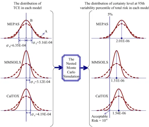
The results of the nested Monte Carlo simulation are shown inTable 3. The risk values of the 50th certainty level and the 95th variability percentile for the total risk estimates computed in MEPAS, MMSOILS, and CalTOX model are 2.01× 10⁻⁶, 1.31× 10⁻⁶, and 1.54× 10⁻⁶, respectively. These risk values are all greater than but close to the pre-assumed acceptable risk level, 10−6.Table 4 lists the important uncertain inputs with contributions to variance of the total risk greater than 5.0%; these
Table 3
The total risk values of 5th, 50th, and 95th certainty level at 5th, 50th, and 95th variability percentile in each model
Variability percentile (%) MEPAS MMSOILS CalTOX
5%a 50%a 95%a 5%a 50%a 95%a 5%a 50%a 95%a
5 4.39E−07 9.14E−07 2.22E−06 2.97E−07 5.89E−07 1.14E−06 3.58E−07 6.96E−07 1.35E−06 50 6.18E−07 1.35E−06 3.10E−06 4.21E−07 8.49E−07 1.61E−06 5.02E−07 1.01E−06 1.97E−06 95 9.24E−07 2.01E−06 4.87E−06 6.33E−07 1.31E−06 2.54E−06 7.53E−07 1.54E−06 3.02E−06
aCertainty level.
Table 4
Major uncertain inputs identified by the sensitivity analysis for the three multimedia risk assessment models
Parameter Definition Contribution to variance of total risk Distribution MEPAS (%) MMSOILS (%) CalTOX (%)
Cwt TCE concentration in groundwater (mg L−1) 54.5 28.9 39.5 Normal (mean = 1.78E−3, S.D. = 6.35E−4) Cwp PCE concentration in groundwater (mg L−1) 17.8 38.4 31.3 Normal (mean = 3.32E−4, S.D. = 1.01E−4) Bvp Soil-to-vegetable transfer factor of PCE (kg/kg) 11.9 15.4 7.8 Lognormal (mean = 1.25, GSD = 2.0) Kpp Skin absorption permeability constant for PCE (cm/h) 6.8 – 10.5 Lognormal (mean = 4.88E−02, GSD = 2.0) Kpt Skin absorption permeability constant for TCE (cm/h) – 5.9 – Lognormal (mean = 4.66E−02, GSD = 2.0) Bvt Soil-to-vegetable transfer factor of TCE (kg/kg) – – 5.2 Lognormal (mean = 1.38, GSD = 2.0)
Table 5
The risk value of 95th certainty level at 95th variability percentile when an input is set at its plausible lower bound or upper bound in various models Parameter Total risk in various models
MEPAS MMSOILS CalTOX
Lower bound Upper bound Lower bound Upper bound Lower bound Upper bound
Cwt 9.25E−07 6.65E−06 7.71E−07 3.67E−06 8.15E−07 4.32E−06
Cwp 2.57E−06 6.43E−06 9.47E−07 2.18E−06 1.19E−06 2.43E−06
Bvp 9.87E−07 3.35E−06 5.13E−07 2.07E−06 6.89E−07 2.78E−06
Kpp 4.89E−06 7.63E−06 – – 2.25E−07 4.03E−06
Kpt – – 1.23E−06 3.19E−06 – –
Bvt – – – – 1.01E−06 2.86E−06
inputs are derived from sensitivity analysis. It is found that the important inputs in different models are similar, although the ranks of influence on the total risk are different, which shows some consistency among these models for the same scenario.
Table 5 shows the analysis results regarding whether the variation of inputs would affect the decision, which is the deter-mination of whether the risk is unacceptable (using 10−6as the criterion in the study) and remediation is needed. It is found that the critical uncertain inputs identified by way of influence on the decision in different models are somewhat different. TCE con-centration in groundwater (Cwt) and soil-to-vegetable transfer factor of PCE (Bvp) are the only two important inputs revealed in
all three models. In addition, PCE concentration in groundwater (Cwp) is a critical uncertain input in the MMSOILS model.
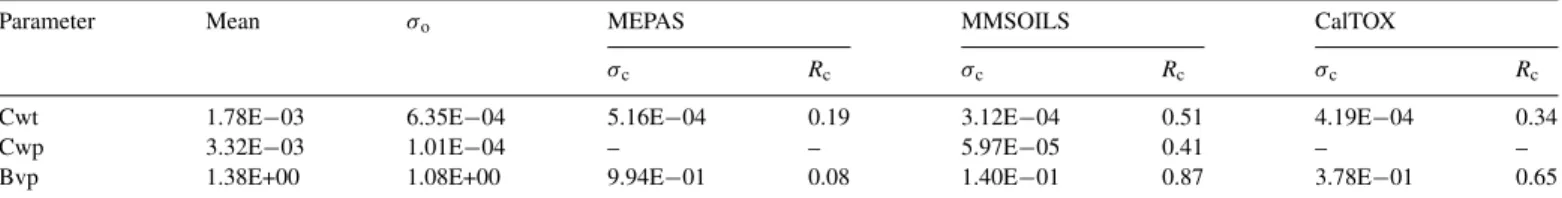
Table 6shows the convergence ratios for the critical uncer-tain inputs identified above (i.e., Cwt, Cwp, and Bvp) to reflect the degree of uncertainty reduction that should be reached to be useful for the decision. Because the total risk values at the 50th certainty level of the 95th variability percentile in the three models are all greater than 10−6, the level of minimum uncer-tainty convergence is reached when the total risk values at the 5th certainty level of the 95th variability percentile are exactly greater than 10−6. As illustrated in Fig. 1, for example, the original distribution of TCE, called A, in the MEPAS model Table 6
The uncertainty convergence ratios needed for avoiding confusion of decision
Parameter Mean σo MEPAS MMSOILS CalTOX
σc Rc σc Rc σc Rc
Cwt 1.78E−03 6.35E−04 5.16E−04 0.19 3.12E−04 0.51 4.19E−04 0.34
Cwp 3.32E−03 1.01E−04 – – 5.97E−05 0.41 – –
Bvp 1.38E+00 1.08E+00 9.94E−01 0.08 1.40E−01 0.87 3.78E−01 0.65
σo: The original standard deviation of each uncertain input;σc: the converged standard deviation of each uncertain input in each model; Rc: the convergence ratio of
Fig. 1. The uncertainty reduction of total risk from the converged distribution of TCE in each model. When the uncertainty of an input is too large (denoted by A) to make a decision, it needs to decrease to be as small as B so that a decision may be made with respect to the decision criteria (e.g., the acceptable risk value 10−6).
spreads over a wide range to make the distribution of total risk covering the decision criteria (e.g., the acceptable risk level of 10−6) and cannot explicitly support the decision. By reducing the input uncertainty of TCE in the MEPAS model, the distri-bution becomes as narrow as B, and the variation of total risk is also reduced to make the 5th percentile risk value of total risk greater than 10−6. In this situation, it becomes clearer that the contaminated site is dangerous enough to require remediation.
As shown inTable 6, the mean and standard deviations of the TCE concentration are 1.78× 10⁻³ and 6.35× 10⁻⁴, respec-tively. In the MEPAS model, the standard deviation of TCE concentration needs to be decreased to 5.16× 10⁻⁴so that the total risk value at the 5th percentile would be greater than 10−6 (the result can also be seen inFig. 1), which produces a con-vergence ratio of 0.19. Therefore, when the TCE concentration is used as the basis to compare the information cost in various models, the order from highest to lowest convergence ratio is as follows: MEPAS, CalTOX, and MMSOILS (the values of the convergence ratio are 0.19, 0.34, and 0.51, respectively, and are shown inTable 6andFig. 1). Because the smaller the conver-gence ratio, the less the reduction of uncertainty needed and the lower the cost of collecting data, the MEPAS model is the best model in this case. Similar results are revealed in the convergence ratios of soil-to-vegetable transfer factor of PCE (these values in the MEPAS, CalTOX, and MMSOILS models are 0.08, 0.65, and 0.87 respectively and are also shown inTable 6). It also indi-cates that the MEPAS is the least costly model for determining whether this site should be further remediated.
When PCE concentration is considered in comparing the information cost in various models, the convergence ratio of PCE concentration in groundwater only in the MMSOILS model is 0.41, while the variation of this input does not influence the decision in either the MEPAS model or the CalTOX model. Therefore, the MEPAS model is the model with the lowest cost of reducing uncertainty to facilitate the decision regarding whether the specific decision criteria (acceptable risk level) is exceeded and the contaminated site should be cleaned up.
In this study, the data collection method of TCE concentration is to sample and analyze more groundwater samples, so the cost of uncertainty reduction is the cost of digging sampling wells, taking samples on-site, and analyzing the samples in the labora-tory. In general, the value of the soil-to-vegetable transfer factor of PCE is obtained from the empirical equation developed by Travis and Arms[39], so if more actual data must be obtained, the cost of analyzing the concentration of several types of vegeta-bles and experimental contaminated soils is needed. Therefore, if different kinds of data collection methods are needed when there are several important inputs involved in selecting a model, the costs of the various data collection methods must be calcu-lated and carefully compared.
5. Conclusion
For a decision problem about whether a contaminated site should be cleaned up, a methodology that combines the cost of reducing uncertainty and the selection of risk assessment
mod-els is developed to facilitate the decision when equally plausible models exist. It is important for a decision maker to make an efficient decision, which entails minimizing costs and maximiz-ing correctness. When the correctness of different models is not easily judged after objective analysis has been conducted, the cost incurred during the processes of risk assessment has to be considered in order to make an efficient decision. When sev-eral models have been used to estimate the risk, the additional cost associated with the decision process would be the cost of ensuring that the modeling results are useful for the decision-making. The proposed methodology enables the identification of efforts involved in reducing the uncertainty of risk estima-tion to the point at which the uncertainty would not hinder the decision-making. Model selection based on this methodology is believed to improve the efficiency of decision. Although the decision problem of site remediation is considered in this study, the methodology can be applied to model selection involved in other decision problems.
Acknowledgements
The study is partly financially supported by Taiwan National Science Council (NSC 94-2621-Z-002-015). The authors would also like to thank the anonymous reviewers for their constructive comments on the earlier version of this manuscript.
References
[1] National Research Council, Risk assessment in the Federal Government: Managing the Process. NAS-NRC Committee on the Institutional Means for Assessment of Risks to Public Health, National Academy Press, Wash-ington, DC, 1983.
[2] H. Ma, Stochastic multimedia risk assessment for a site with contaminated groundwater, Stochastic Environ. Res. Risk Assess. 16 (2002) 464–478. [3] R.M. Maxwell, W.E. Kastenberg, Stochastic environmental risk analysis:
an integrated methodology for predicting cancer risk from contaminated groundwater, Stochastic Environ. Res. Risk Assess. 13 (1999) 27–47. [4] M.G. Morgan, M. Henrion, Uncertainty: A Guide to Dealing with
Uncer-tainty in Quantitative Risk and Policy Analysis, Cambridge University Press, New York, 1990.
[5] A.M. Finkel, Confronting Uncertainty in Risk Management: A Guide for Decision-Makers, Center for Risk Management Resources for the Future, Washington, DC, 1990.
[6] USEPA, Guidelines for Exposure Assessment, Office of Health and Envi-ronmental Assessment, Washington, DC, 1992.
[7] H.C. Frey, Quantitative Analysis of Variability and Uncertainty in Envi-ronmental Policy Making, American Association for the Advancement of Science, Washington, DC, 1992.
[8] A.C. Cullen, H.C. Frey, Probabilistic Techniques in Exposure Assessment, Plenum Press, New York, 1999.
[9] G.J. Klir, M.J. Wierman, Uncertainty-Based Information, Physica-Verlag, New York, NY, 1999.
[10] A.E. Smith, P.R. Ryan, J.S. Evans, The effect of neglecting correlation when propagating uncertainty and estimating the population distribution of risk, Risk Anal. 12 (1992) 467–474.
[11] A.C. Taylor, Using Objective and subjective information to develop distri-butions for probabilistic exposure assessment, J. Exposure Anal. Environ. Epidemiol. 3 (1993) 285–298.
[12] T.E. Mckone, Uncertainty and variability in human exposures to soil con-taminants through home-grown food-A Monte-Carlo assessment, Risk Anal. 14 (1994) 449–463.
[13] R.L. Maddalena, T.E. Mckone, D.P.H. Hsieh, S. Geng, Influential input classification in probabilistic multimedia models, Stochastic Environ. Res. Risk Assess. 15 (2001) 1–17.
[14] T.E. Mckone, K.T. Bogen, Predicting the uncertainties in risk assessment—a California groundwater case-study, Environ. Sci. Technol. 25 (1991) 1674–1681.
[15] R.M. Maxwell, S.D. Pelmulder, A.F.B. Tompson, W.E. Kastenberg, On the development of a new methodology for groundwater-driven health risk assessment, Water Resour. Res. 34 (1998) 833–847.
[16] D.J. Moschandreas, S. Karuchit, Scenarion-model-parameter: a new method of cumulative risk uncertainty analysis, Environ. Int. 28 (2002) 247–261.
[17] E.G. Hertwich, T.E. Mckone, W.S. Pease, A systematic uncertainty anal-ysis of an evaluate fate and exposure model, Risk Anal. 20 (2000) 439– 454.
[18] D. Pollock, R. Salama, R. Kookana, A study of atrazine transport through a soil profile on the Gnangara Mound, Western Australia, using LEACHP and Monte Carlo techniques, Aust. J. Soil Res. 40 (2002) 455–464. [19] F.O. Hoffman, J.S. Hammonds, Propagation of uncertainty in risk
assess-ments: the need to distinguish between uncertainty due to lack of knowledge and uncertainty due to variability, Risk Anal. 14 (1994) 707–712. [20] G.F. Laniak, J.G. Droppo, E.R. Faillance, E.K. Gnanapragasam, W.B.
Mills, D.L. Strenge, G. Whelan, C. Yu, An overview of a multimedia bench-marking analysis for three risk assessment models: RESRAD, MMSOILS, and MEPAS, Risk Anal. 17 (1997) 203–214.
[21] W.B. Mills, J.J. Cheng, J.G. Droppo, E.R. Faillance, E.K. Gnanapragasam, R.A. Johns, G.F. Laniak, C.S. Lew, D.L. Strenge, J.F. Sutherland, G. Whelan, C. Yu, Multimedia benchmarking analysis for three risk assess-ment models: RESRAD, MMSOILS, and MEPAS, Risk Anal. 17 (1997) 187–201.
[22] J.L. Regens, K.R. Obenshian, C. Travis, C. Whipple, Conceptual site models and multimedia modeling: comparing MEPAS, MMSOILS, and RESRAD, Human Ecol. Risk Assess. 8 (2002) 391–403.
[23] G. Whelan, J.P. McDonald, E.K. Gnanapragasam, G.F. Laniak, C.S. Lew, W.B. Mills, C. Yu, Benchmarking of the vadose-zone module associated with three risk assessment models: RESRAD, MMSOILS, and MEPAS, Environ. Eng. Sci. 16 (1999) 81–91.
[24] W.E. Fayerweather, J.J. Collins, R. Schnatter, F.T. Hearne, R.A. Menning, D.P. Reyner, Quantifying uncertainty in a risk assessment using uncertainty data, Risk Anal. 19 (1999) 1077–1090.
[25] J.S. Evans, J.D. Graham, G.M. Gray, R.L. Sielken Jr., A distributional approach to characterizing low-dose cancer risk, Risk Anal. 14 (1994) 24–34.
[26] Y. Chen, H. Ma, Model comparison for risk assessment: a case study of contaminated groundwater, Chemosphere 63 (2006) 751–761.
[27] E.P.A. Taiwan, The Evaluative and Analytic Principles of Health Risk Assessment, Soil and Groundwater Remediation Fund Management Board, Taipei, Taiwan, 2005 (in Chinese).
[28] J.W. Buck, G. Whelan, J.G. Droppo, K.L. Strenge, K.J. Castleton, J.P. McDonald, C. Sato, G.P. Streile, Multimedia Environmental Pollutant Assessment System (MEPAS) Application Guidance, Guidelines for Eval-uating MEPAS Input Parameters for version 3.1, Pacific Northwest Labo-ratory, Richland, Washington, 1995.
[29] USEPA, MMSOILS Model: Multimedia Contaminated Fate, Transport, and Exposure Model: Documentation and User’s Manual Version 4.0, Office of Research and Development, Washington, DC, 1996.
[30] T.E. Mckone, CalTOX: A Multimedia Total-Exposure Model for Haz-ardous Waste Sites. Part I. Executive Summary, Department of Toxic Substances Control, Lawrence Livermore National Laboratory, Livemore, California, 1993.
[31] T.E. Mckone, CalTOX: A Multimedia Total-Exposure Model for Haz-ardous Waste Sites. Part II. Multimedia Transport and Transformation Model, Department of Toxic Substances Control, Lawrence Livermore National Laboratory, Livemore, California, 1993.
[32] T.E. Mckone, CalTOX: A Multimedia Total-Exposure Model for Haz-ardous Waste Sites. Part III. Multipathway Exposure Model, Department of Toxic Substances Control, Lawrence Livermore National Laboratory, Livemore, California, 1993.
[33] A. Mokhtari, H.C. Frey, Sensitivity analysis of a two-dimensional prob-abilistic risk assessment model using analysis of variance, Risk Anal. 25 (2005) 1511–1529.
[34] A. Mokhtari, H.C. Frey, Recommended practice regarding selection of sensitivity analysis methods applied to food safety risk process models, Human Ecol. Risk Assess. 11 (2005) 591–605.
[35] J.C. Helton, F.J. Davis, Illustration of sampling-based methods for uncer-tainty and sensitivity analysis, Risk Anal. 22 (2002) 591–622.
[36] A. Saltelli, Sensitivity analysis for importance assessment, Risk Anal. 22 (2002) 1–12.
[37] T.E. Mckone, Alternative modeling approaches for contaminant fate in soils: uncertainty, variability, and reliability, Reliab. Eng. Syst. Saf. 54 (1996) 165–181.
[38] H. Ma, Setting information priorities for remediation decisions at a contaminated-groundwater site, Chemosphere 46 (2002) 75–81.
[39] C.C. Travis, A.D. Arms, Bioconcentration of organics in beef, milk, and vegetation, Environ. Sci. Technol. 22 (1988) 271–274.
[40] California EPA, CalTOX: A Multimedia Total-Exposure Model for Haz-ardous Waste Sites, Sacramento, 1993.
[41] J.A. Droppo, G. Whelan, J.W. Buck, D.L. Strenge, Supplemental Math-ematical Formulations: The Multimedia Environmental Pollutant Assess-ment System (MEPAS), Pacific Northwest Laboratory, Richland, Wash-ington, 1989.
[42] H.C. Yeh, W.E. Kastenberg, Health risk assessment of biodegradable volatile organic chemicals: a case study of PCE, TCE, DCE and VC, J. Hazard. Mater. 27 (1991) 111–126.
[43] M. Kao, M. Tsan, W. Yeh, Health and obesity of Taiwan citizens, Chin. Nutr. J. 22 (1997) 143–171 (in Chinese).
[44] S. Wu, Y. Chang, C. Fang, W. Pan, Food sources of weight, calories and three macro-nutrients: NAHSIT 1993–1996, Nutr. Sci. J. 24 (1999) 59–80.