A Study for Insolvency in the Life Insurance Industry of Taiwan

全文

(1)A Study for Insolvency in the Life Insurance Industry of Taiwan. James C. Hao* Lin-Yhi Chou**. Abstract The study employs factor analysis and logistic regression (FAST approach) to estimate the probabilities of insolvency of Taiwan’s life insurers. Our findings show that changes in the fixed asset ratio, changes in the liquid asset ratio, and changes in loan ratio are important factors for Taiwanese life insurers’ insolvency. Therefore, the commissioner should focus on these financial ratios. This study presents that almost 10 percent of life insurers in Taiwan have a problem of insolvency. Keyword: Financial Analysis and Solvency Tracking system, Factor analysis, Logistic regression, Multidiscriminant analysis, Probabilities of insolvency.. 1. Introduction The prediction of financial insolvency for life insurance companies is a major concern of insurance consumers and regulators in Taiwan. For the life insurers, three firms have shown the problem of insolvency in the last decade, making it a major issue for Taiwan’s insurance commissioners. In the last decade Taiwan life insurance industry did not have one case of bankruptcy, because the commissioners played the role of matchmaker in seeking potential mergers for taking over insolvent companies and improving those companies’ capital adequacy ratio. Thus, the island’s life insurance industry only had one quasi-insolvency case in the past decade when the Hontai Life took over Hung FU Life Insurance in 1999. Although the combined company exists right now, the ownership of it has been already transformed.. *. Associate Professor, Department of Insurance, Tamkang University. E-mail: cjhao@mail.tku.edu.tw Ad d r e s s : 1 5 1 Y i n g - c h u a n R o a d T a i p e i H s i e n , T a i wa n R . O C . Tel: 886-2-26215656 ext 2561. **. L.Y. Chou is a Ph.D student, College of Business, Feng Chia University, Taichung... 第五屆全國實證經濟學論文研討會 The 5th Annual Conference of Taiwan's Economic Empirics.

(2) Kuo-Hua Life Insurance, which the market share of it was above 5 percent at that time, stopped its business operation in 2000 because the company’s capital adequacy ratio was lower than the regulation level. From Figure 1, we find that the capital to reserve ratio for Kuo-Hua in 2000 at 2.02% was the lowest in Taiwan’s life insurance industry. Because of these events, the insurance commissioners began to focus on the issue of life insurance company insolvency. 66%. 62%772%. Capital-Reserve Ratio. 459%. 46%. 45%. 41%. 40%. 39% 33%. 35%. 30%. 30%. 23%. 25%. 20%. 20%. 20%. 16%. 15% 10%. 68% 64%. 173%. 89% 48%. 50%. 18%. 22% 16%. 13%. 9% 5%. 5%. 6%. 3%. 3% 2.02%. 5%. 0% 1. 2. 3. 4. 5. 6. 7. 8. 9. 10 11 12 13 14 15 16 17 18 19 20 21 22 23 24 25 26 27 28 29. Firm. Figure 1. Taiwanese life insurance firms’ capital-reserve ratio in 2000. In Figure 2 the capital-reserve ratio for Taiwan’s life insurance industry decreased from 1997 to 2001. The lowest rate for the growth in the capital-reserve ratio at –10.25% occurred in 2000. Thus, we can easily predict that solvency in this industry decrease, making it a major concern for Taiwan’s insurance commissioners in the next decade.. Growth of Capital-Reserve ratio. 0%. -2%. -4%. -6%. -8%. -10%. -12% 1997. 1998. 1999. 2000. 2001. Year. Figure 2.. Taiwan’s life insurance industry growth in capital-reserve ratio from 1997 to 2000. Up until to now, Taiwan’s insurance commissioners have developed an Insurance Regulatory Information System (IRIS), Financial Analysis and Solvency Tracking System (FAST), and Risk Based Capital (RBC) systems to test the probability of insolvency for life insurance companies. Therefore, we employ public information to estimate the probability of insolvency for 29 firms in Taiwan. -2第五屆全國實證經濟學論文研討會 The 5th Annual Conference of Taiwan's Economic Empirics.

(3) In past research studies, many authors found that the NAIC system is not a reliable predictor of insolvency for life insurers. (Breslin and Troxel, 1978; Thornton and Meador, 1977; Hershbarger, 1981; Hershbarger and Miller, 1986; Barniv and Hershbarger, 1990). Some authors proved that the Financial Analysis and Solvency Tracking System (FAST) has more efficiency in predicting the financial insolvency of life insurance companies (Barniv and Hershbarger, 1990; Carson and Hoyt, 1995). Therefore, we employ the FAST approach to estimate the insolvency issue in Taiwan. The remainder of the paper is organized as follows: a brief review of the insolvency issue is presented in section 2. Section 3 explains methodology and section 4 describes the estimation and results. Summary and conclusion are presented in section 5.. 2. Literature Review Altman (1968) was the first scholar who employed financial ratios to estimate the issue of property insurance insolvency. After that, three similar approaches were developed: Mulitidiscriminant analysis(MDA) (Trieschmann and Pinches, 1973; 1974; Harmelink, 1974; Hershbarger and Miller, 1986; Ambrose and Seward, 1988; Carson and Hoyt, 1995), logistic regression approach (Ohlson, 1980; Zmijewskim, 1984; Barniv, 1990; 1992, Ambrose and Carroll, 1994; Cummins et al., 1995; Cummins et al., 1999), and Back-Propagation Network (BPN)(Huang et al, 1995; Lin, 1996). Barniv et al. (1999) improved the logistic regression model that adopts the interval estimate. They also claimed that the logistic model is a preferred method in their study as some important distributional assumptions under MDA are violated, and the MDA estimators are inconsistent if the independent variables are not normally distributed, as is the study when dummy variables are used (Ohlson, 1980; Maddala, 1983; Barniv and McDonald, 1992). Radcliffe (1982) pointed out that all the margins of life and health insurers have disappeared. Belth (1984) argued that it is possible for large life insurers to run into financial distress, and that the consequence of such failures is in terms of a loss of public confidence in life insurers. Granger et al. (1987) indicated that a change in economic conditions and industries factors (such as increase demand for policy loans) are the possible causes of crises, and they employed decomposition analysis to find the failure for life insurers one year prior to insolvency. Cheong et al.(1988) employed factor analysis for variable selection. Barniv and Hershbarger (1990) found that a change in product mix and profitable operations and investment are important factors of insolvency. Carson and Hoyt (1995) indicated that equity to debit, natural log of cash flow, bonds plus mortgages to assets, and a change in premium are the important factors. Lin (1996) showed that -3第五屆全國實證經濟學論文研討會 The 5th Annual Conference of Taiwan's Economic Empirics.

(4) the important factor is a profitable variable. Kao and Chan (2001) found that the liquid ratio, debit ratio, expense ratio, and market share are the important factors of insolvency. Shaked’s (1985) findings are that large life insurance firms are reasonably safe, but the distribution of the probability of failure is skewed to the right. Thus, a few life insurers pose greater insolvency risk than others in his sample. Therefore, we employ the logistic regression to predict the probability of insolvency and factor analysis for variable selection.. 3. Methodology 3.1 Data Source Twenty-nine firms operating in Taiwan’s life insurance market during 1997~2001 were gathered for this study. We obtained data from the Life Insurance Association of the Republic of Taiwan. 3.2 Logistic Model The coefficients of the independent variables are derived by conditional probability models through a dichotomous dependent variable (Y). Either the logistic or the probit models might derive the cumulative distribution. The life insurer insolvency probability is expressed by P (y=1): e β 0 + xβ1 1 = (1) P( y = 1) = β 0 + x β1 − ( β 0 + xβ1 ) 1+ e 1+ e where Y is zero or 1; 1 is an insolvent firm; X is an independent variables; and β is a coefficient. The term P (y) is a probability value derived from equation (1). P ( y i ) = Pi yi (1 − Pi )1− yi (2). where P (y) is the joint probability distribution and is expressed by equation (3). n. L(θ ) = ∏ Pi yi (1 − Pi )1− yi (3) i =1. where the logistic regression maximum likelihood estimation is equation (4). n. ln[ L(θ )] = ln[∏ Pi yi (1 − Pi )1− yi ] i =1. n. = ∑ [ y i ln( pi ) + (1 − y i ) ln(1 − pi )] i =1 n. = ∑ { y i (α + βxi ) − ln(1 + eα + βxi )} (4) i =1. Here, P (y) represents the probabilities of insolvency and y i = α + βxi . 3.3 MDA Model The function is of the form: -4第五屆全國實證經濟學論文研討會 The 5th Annual Conference of Taiwan's Economic Empirics.

(5) P(Y = 1) = β 0 + β 1 X (5) where Y is a dummy variable (1 is insolvency; 0 is others), β are coefficients, and X are factor scores. 3.4 Factor Analysis The procedures are the following. First, we take a proportion of each financial ratio. Second, we employ a weight by the proportion of structure loading and calculate the factor score (X). Third, the factor score is substituted into equation (1).. Z ik − Min ) × 100 × weight (6) Max − Min where S expresses the i financial score of the k firm and Z is the i financial ratio of the k firm. The proportion of the structure loading is equation (7). S ik = (. Tk =. α kj2 ∑ α kj 2. (7). where T is the weight, αis k firm, and j the structure loading. The structure loadings are calculated from equation (8). Z ij = α ij1 F1ij + α ij 2 F2ij + ...... + α ijk FKij + d j µ ji (8). where Z ij expresses the j variable of the i firm.. Term FKij is a k factor. coefficient of the j variable from the i firm. Term α Kij is the k structure loading of the j variable from the i firm. Term µ ji is an independent loading and d j is the coefficient of the independent loading. The maximum of the loading variance approach is employed to set a structure. 3.5 Financial Ratio Ten financial ratios from FAST are employed.. Change in capital and surplus (CSC) Carson, et al (1996) indicated that the companies with higher capital to back their increased bank-type exposures tend to be rewarded with higher ratings. This ratio is a measure of capital and surplus. Generally, this ratio is estimated by equation (9). S − S t −1 CS = t (9) S t −1. S t −1. where CS is the change in capital and surplus, S t is capital and surplus in t, and is capital and surplus in t-1. Change in Premium (PC) This ratio is a measure of stable business line growth. The larger the ratio is, the -5第五屆全國實證經濟學論文研討會 The 5th Annual Conference of Taiwan's Economic Empirics.

(6) less the probability will be of insolvency (Ambrose and Carroll, 1994; Pottier, 1998). This ratio is estimated by equation (10). P − Pt −1 CP = t (10) Pt −1 where CP is the change in total premium, Pt is the total premium in t, and Pt −1 is the total premium in t-1. Accident and Health Business to Total Premium (AHR) The larger this ratio is, the more expected probability there will be of insolvency. We expect a positive coefficient. Change in Profit (PRC) This ratio is a measure of profitability. Both underwriting and investment returns are included. The firm which has larger profits tends to have less probability of insolvency (Ambrose and Carroll, 1994; Pottier, 1998). Change in Liquid Asset (LAC) Carson, et al. (1996) indicated that life insurers that have greater liquidity to back deposit-like liabilities are expected to receive higher ratings. Liquidity is measured by the ratio of cash plus other short-term investments to total investments in financial assets. We expect a negative coefficient. Change in Fixed Assets (FAC) The change in fixed assets, which can be used to measure liquidity, is correlated to the change in liquid assets. The firm which has a larger percentage of fixed assets tends to have more probability of insolvency. Operation Size (LTA) The nature log of total assets is used to measure operation size. Rapidly growing companies are more vulnerable to financial distress (Shaked, 1985; Barniv and Hershbarger, 1990; Carson, et al, 1996; Pottier, 1998), but some authors indicate that the larger the operation size is, the more decentralized the risk will be for Taiwan’s insurers (Chen and Tsai, 2002;Shiu and Wang, 2003). Therefore, we expect a negative coefficient. Change in Reserves (REC) This ratio is used to measure the stability of operations. If this ratio is larger, then the firm’s cash flow will encounter large distress and the expected probability of insolvency is larger. Change in Reinsurance Ratio (RINC) The reinsurance ratio is the ratio in which claims receivable from reinsurance are divided into the benefits paid to policyholders. Therefore, we assume that the ratio is negatively correlated to the expected probability of insolvency.. -6第五屆全國實證經濟學論文研討會 The 5th Annual Conference of Taiwan's Economic Empirics.

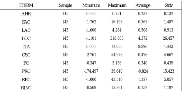
(7) Change in Loan Ratio (LOC) The loan ratio is the ratio of the number of loans divided by the amount of total assets. If this ratio changes too quickly, then the firm may suffer more credit risk. Therefore, we assume that this ratio is positively correlated to the expected probability of insolvency.. 4. Estimation and Results We employ the logistic model and factor analysis to estimate the insolvency of 29 life insurance companies from 1997 to 2001. The data come from the Life Insurance Association of the Republic of Taiwan. 4.1 Data statistical and Correlation Analysis Table 1. The statistical data. ITERM. Sample. Minimum. Maximum. Average. Stdv. AHR. 145. 0.036. 0.731. 0.232. 0.132. FAC. 145. -1.762. 16.193. 0.367. 1.487. LAC. 145. -1.000. 4.284. 0.508. 0.913. LOC. 145. -1.101. 318.883. 4.372. 26.457. LTA. 145. 0.000. 12.055. 9.896. 1.443. CSC. 145. -2.761. 54.978. 0.476. 4.667. PC. 145. -0.347. 3.156. 0.340. 0.439. PRC. 145. -174.497. 39.640. -0.824. 15.423. REC. 145. -1.000. 43.310. 1.227. 5.057. RINC. 145. -0.509. 13.361. 0.152. 1.197. * We obtained data from the Life Insurance Association of the Republic of Taiwan. In Table 1 we find that the change in the loan ratio is growing quickly, and change in profits is negatively affected. Thus, it means that life insurers in Taiwan are more vulnerable to credit risk and more operation risk. Table 2 Correlation AHR AHR. FAC. LAC. LOC. LTA. CSC. PC. 1.000 -. FAC. LAC. LOC. -0.031. 1.000. (0.354). -. -0.089. 0.128. 1.000. (0.143). (0.063). -. -0.022. 0.916. 0.141. 1.000. (0.396). (0.000). (0.046)*. -. -7第五屆全國實證經濟學論文研討會 The 5th Annual Conference of Taiwan's Economic Empirics. PRC. REC. RINC.

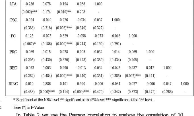
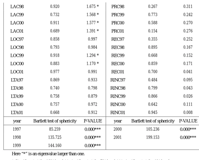
(8) LTA. -0.236. 0.078. 0.194. 0.068. 1.000. (0.002)***. 0.174. (0.010)**. 0.208. -. -0.024. -0.040. 0.226. -0.034. 0.037. 1.000. (0.388). (0.318). (0.003)***. (0.340). (0.327). -. 0.125. -0.075. 0.329. -0.058. -0.073. -0.046. 1.000. (0.067)*. (0.186). (0.000)***. (0.244). (0.190). (0.291). -. -0.069. 0.015. 0.028. 0.005. 0.032. 0.014. 0.069. 1.000. (0.205). (0.430). (0.370). (0.478). (0.350). (0.434). (0.205). -. -0.053. 0.003. 0.290. -0.013. 0.032. -0.025. 0.237. 0.012. 1.000. (0.262). (0.484). (0.000)***. (0.440). (0.351). (0.385). (0.002)***. (0.441). -. 0.010. 0.886. 0.101. 0.920. -0.006. -0.034. 0.027. -0.006. 0.047. 1.000. (0.453). (0.000)***. (0.114). (0.000)***. (0.470). (0.342). (0.373). (0.472). (0.286). -. CSC. PC. PRC. REC. RINC. 1.. * Significant at the 10% level ** significant at the 5% level *** significant at the 1% level.. 2.. Here (*) is P-Value.. In Table 2 we use the Pearson correlation to analyze the correlation of 10 financial ratios. We find that operation size is negatively correlated to the accident and health business ratio. The change in the fixed asset ratio with the reinsurance ratio is positively related. 4.2 Factors Analysis Factor Select and Loading In Table 3 we find that the accident and health business ratio, change in fixed asset ratio, change in liquid asset ratio, and change in loan ratio are important factors on Taiwan life insurers’ insolvency. Kao and Chan (2001) indicated that a change in the liquid asset ratio is an important factor for Taiwan life insurers’ insolvency. Table 3 Factor analysis Variable. Loading. Eigenvalue. Variable. Loading. Eigenvalue. AHR97. 0.729. 3.213 *. CSC97. 0.621. 0.751. AHR98. 0.743. 3.157 *. CSC98. 0.632. 0.467. AHR99. 0.335. 2.890 *. CSC99. 0.803. 0.679. AHR00. 0.309. 2.778 *. CSC00. 0.881. 0.723. AHR01. 0.494. 2.995 *. CSC01. 0.305. 0.660. FAC97. 0.602. 1.545 *. PC97. 0.334. 0.628. FAC98. 0.502. 2.015 *. PC98. 0.554. 0.383. FAC99. 0.956. 1.893 *. PC99. 0.835. 0.378. FAC00. 0.663. 1.824 *. PC00. 0.858. 0.404. FAC01. 0.987. 2.296 *. PC01. 0.764. 0.430. LAC97. 0.589. 1.096 *. PRC97. 0.413. 0.491. -8第五屆全國實證經濟學論文研討會 The 5th Annual Conference of Taiwan's Economic Empirics.

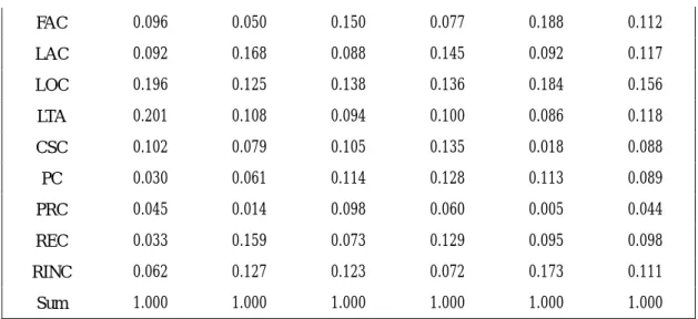
(9) LAC98. 0.920. 1.675 *. PRC98. 0.267. 0.311. LAC99. 0.732. 1.568 *. PRC99. 0.773. 0.242. LAC00. 0.911. 1.577 *. PRC00. 0.588. 0.270. LAC01. 0.689. 1.391 *. PRC01. 0.154. 0.276. LOC97. 0.858. 0.997. REC97. 0.355. 0.252. LOC98. 0.793. 0.984. REC98. 0.895. 0.167. LOC99. 0.918. 1.294 *. REC99. 0.668. 0.152. LOC00. 0.883. 1.170 *. REC00. 0.859. 0.171. LOC01. 0.977. 0.991. REC01. 0.700. 0.041. LTA97. 0.869. 0.933. RINC97. 0.484. 0.095. LTA98. 0.740. 0.798. RINC98. 0.799. 0.043. LTA99. 0.758. 0.879. RINC99. 0.866. 0.026. LTA00. 0.757. 0.972. RINC00. 0.642. 0.111. LTA01. 0.668. 0.912. RINC01. 0.945. 0.008. year. Bartlett test of sphericity. P-VALUE. year. Bartlett test of sphericity. P-VALUE. 1997. 85.259. 0.000***. 2000. 105.236. 0.000***. 1998. 135.725. 0.000***. 2001. 199.153. 0.000***. 1999. 144.160. 0.000***. 1.. Here “*” is an eigenvalue larger than one.. 2.. * Significant at the 10% level ** significant at the 5% level *** significant at the 1% level.. 3.. Bartlett test of sphericity is H 0 : R p = 1 , H 1 : R p ≠ 1 .. If R=1, then we don’t employ the factor. analysis for this empirical study.. Weight We use equation (7) to estimate the weight and find that the loading of change in the fixed asset ratio, change in liquid asset ratio, change in loan ratio, operation size, and change in reinsurance ratio are more important than other factors (In Table 4). In the past decade, the life insurers didn’t pay attention to reinsurance, because they believed that their capacities were enough to cover all business lines. Because one incumbent life insurer was close to bankrupcy in 1997, the life insurers began to understand that reinsurance is very importance in order to decentralize risk. The insolvency and cash flow of a life insurer is affected by a change in the fixed ratio and liquid assets. The larger the fixed asset ratio is, the less liquid the life insurer is. Table 4 Structure loading (weight) Variable. 1997. 1998. 1999. 2000. 2001. Average. AHR. 0.141. 0.109. 0.018. 0.017. 0.047. 0.067. -9第五屆全國實證經濟學論文研討會 The 5th Annual Conference of Taiwan's Economic Empirics.

(10) FAC. 0.096. 0.050. 0.150. 0.077. 0.188. 0.112. LAC. 0.092. 0.168. 0.088. 0.145. 0.092. 0.117. LOC. 0.196. 0.125. 0.138. 0.136. 0.184. 0.156. LTA. 0.201. 0.108. 0.094. 0.100. 0.086. 0.118. CSC. 0.102. 0.079. 0.105. 0.135. 0.018. 0.088. PC. 0.030. 0.061. 0.114. 0.128. 0.113. 0.089. PRC. 0.045. 0.014. 0.098. 0.060. 0.005. 0.044. REC. 0.033. 0.159. 0.073. 0.129. 0.095. 0.098. RINC. 0.062. 0.127. 0.123. 0.072. 0.173. 0.111. Sum. 1.000. 1.000. 1.000. 1.000. 1.000. 1.000. Factors Score Equation (6) is employed to estimate factors scores. In Table 5, four firms, with their stability among the top 13.79 percent of the industry, belong to a degree of B. Ten firms belong to a degree of C+, while thirteen firms are degree of C-. According to our definition, D and E are poorly stable and insolvent, and one firm belongs to a degree of D and one firm belongs to E, and these dangerous firms amount to 6.9 percent of the whole industry. Therefore, we think that Taiwan’s insurance commissioners should pay more attention on these firms. Table 5 The factor scores Degree. 1997. 1998. 1999. 2000. 2001. Average. Formula. Amount of Firms. A. 2.941. 3.693. 4.153. 4.915. 2.808. 3.702. µ − 1 .5 × σ. 0. 0.00%. B. 3.669. 4.191. 4.817. 5.572. 3.412. 4.332. µ − 0.5 × σ. 4. 13.79%. C+. 4.034. 4.441. 5.149. 5.900. 3.715. 4.647. µ. 10. 34.48%. C-. 4.398. 4.690. 5.481. 6.228. 4.017. 4.963. µ + 0 .5 × σ. 13. 44.83%. D. 5.126. 5.189. 6.144. 6.884. 4.621. 5.593. µ + 1 .5 × σ. 1. 3.45%. 1. 3.45%. E 1.. Percentage. D PLUS D PLUS D PLUS D PLUS D PLUS D PLUS. Here, “μ” expresses the mean of factor score in the current year, and “σ” expresses the standard variance of the factor score in the current year.. 2.. The term A expresses the firm has the largest stable degree, B expresses the firm of more stable degree, C+ is stable, C- is less stable, D is poorly stable (dangerous), and E means that the firm is insolvent.. 4.3 Empirical Study on Logistic and MDA Model Equations (1) and (5) are employed to estimate the probability of insolvency, and the variable which we use is a factor score. From 1997 to 2000, the goodness of fit test (Hosmer-Lemeshow) is adopted to test the homogeneity of the sample. In 2001 two firms were on the stop business line, and therefore we think that the sample has - 10 第五屆全國實證經濟學論文研討會 The 5th Annual Conference of Taiwan's Economic Empirics.

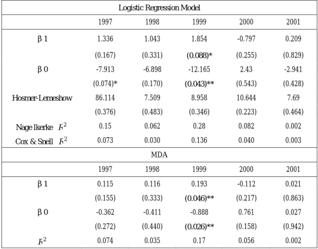
(11) some degree of heterogeneity. We find that the coefficient is significantly positive to the dummy variable of degree of D. Therefore, we employ factors which have a contribution to probabilities of insolvency. We can now employ the logistic regression and MDA model coefficient to estimate the probability of insolvency. Table 6 Logistic regression and MDA model Logistic Regression Model 1997. 1998. 1999. 2000. 2001. 1.336. 1.043. 1.854. -0.797. 0.209. (0.167). (0.331). (0.088)*. (0.255). (0.829). -7.913. -6.898. -12.165. 2.43. -2.941. (0.074)*. (0.170). (0.043)**. (0.543). (0.428). 86.114. 7.509. 8.958. 10.644. 7.69. (0.376). (0.483). (0.346). (0.223). (0.464). Nage lkerke R 2. 0.15. 0.062. 0.28. 0.082. 0.002. Cox & Snell R 2. 0.073. 0.030. 0.136. 0.040. 0.003. β1. β0. Hosmer-Lemeshow. MDA. β1. β0. R2. 1997. 1998. 1999. 2000. 2001. 0.115. 0.116. 0.193. -0.112. 0.021. (0.155). (0.333). (0.046)**. (0.217). (0.863). -0.362. -0.411. -0.888. 0.761. 0.027. (0.272). (0.440). (0.026)**. (0.158). (0.942). 0.074. 0.035. 0.17. 0.056. 0.002. 1.. * Significant at the 10% level ** significant at the 5% level *** significant at the 1% level.. 2. 3.. Here X represents factor scores in the current Year. Here, βis a coefficient by equation (1).. In table 7 we use the logistic model to estimate the probability of insurer insolvency. The average probability of insolvency for life insurers is 10.34 percent, which means that 10.34 percent of firms are dangerous by the logistic model. In this study we find that the change in the fixed asset ratio, change in liquid asset ratio, and changes in the loan ratio are important factors of Taiwanese life insurers’ insolvency (In Table 4). The change in the fixed asset ratio and changes in liquid asset ratio are always significant for the insolvency study (Carson and Hoyt, 1995). Thus the commissioner can employ these ratios to predict the probability of insolvency. Kao and Chan (2001) indicated that the change in liquid asset ratio is an important factor for Taiwanese life insurers’ insolvency, and we also have the same result. - 11 第五屆全國實證經濟學論文研討會 The 5th Annual Conference of Taiwan's Economic Empirics.

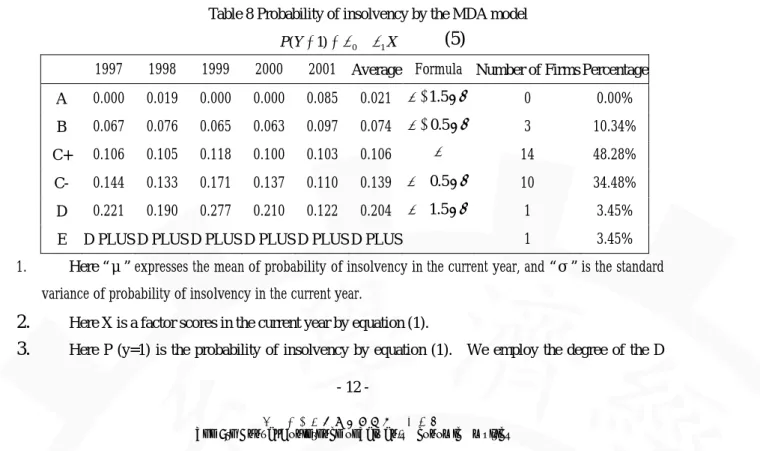
(12) Table 7. Probability of insolvency by the logistic model. P( y = 1) = Degree. 1997. 1998. e β 0 + xβ1 1 = β 0 + xβ1 − ( β 0 + xβ1 ) 1+ e 1+ e. 1999. 2000. 2001. (1). Average. Amount of. Formula. Firms. Percentage. A. 0.000. 0.013. 0.000. 0.000. 0.085. 0.020. µ − 1 .5 × σ. 0. 0.00%. B. 0.057. 0.073. 0.028. 0.065. 0.097. 0.064. µ − 0.5 × σ. 2. 6.90%. C+. 0.103. 0.103. 0.103. 0.103. 0.103. 0.103. µ. 16. 55.17%. C-. 0.149. 0.134. 0.179. 0.142. 0.110. 0.143. µ + 0 .5 × σ. 8. 27.59%. D. 0.241. 0.194. 0.329. 0.218. 0.122. 0.221. µ + 1 .5 × σ. 2. 6.90%. 1. 3.45%. E 1.. D PLUS D PLUS D PLUS D PLUS D PLUS D PLUS. Here “μ” expresses the mean of probability of insolvency in the current year, and “σ” expresses the standard variance of probability of insolvency in the current year.. 2.. Here X is a factor scores in the current year by equation (1).. 3.. Here P (y=1) is the probability of insolvency by equation (1), where we employ the degree of the D firm to substitute for an actual insolvent firm.. 4.. We set apart the degree from A to E. The term A expresses that the firm has the most stable degree, B has a more stable degree, C+ is stable, C- is less stable, D is poorly stable (dangerous), and E is insolvent.. In Table 8, we employ MDA to estimate the probability of insolvency, and the average probability of insolvency for a life insurer is10.6percent, which means that 10.6 percent of firms is dangerous by the MDA model. When we compare the logistic model with MDA, we find that a pessimistic result from the MDA model. Table 8 Probability of insolvency by the MDA model P (Y = 1) = β 0 + β 1 X. 1997. 1998. 1999. 2000. 2001. A. 0.000. 0.019. 0.000. 0.000. 0.085. 0.021. µ − 1 .5 × σ. 0. 0.00%. B. 0.067. 0.076. 0.065. 0.063. 0.097. 0.074. µ − 0.5 × σ. 3. 10.34%. C+. 0.106. 0.105. 0.118. 0.100. 0.103. 0.106. µ. 14. 48.28%. C-. 0.144. 0.133. 0.171. 0.137. 0.110. 0.139 µ + 0.5 × σ. 10. 34.48%. D. 0.221. 0.190. 0.277. 0.210. 0.122. 0.204. µ + 1 .5 × σ. 1. 3.45%. 1. 3.45%. E 1.. (5). Average Formula Number of Firms Percentage. D PLUS D PLUS D PLUS D PLUS D PLUS D PLUS. Here “μ” expresses the mean of probability of insolvency in the current year, and “σ” is the standard variance of probability of insolvency in the current year.. 2. 3.. Here X is a factor scores in the current year by equation (1). Here P (y=1) is the probability of insolvency by equation (1). We employ the degree of the D - 12 第五屆全國實證經濟學論文研討會 The 5th Annual Conference of Taiwan's Economic Empirics.

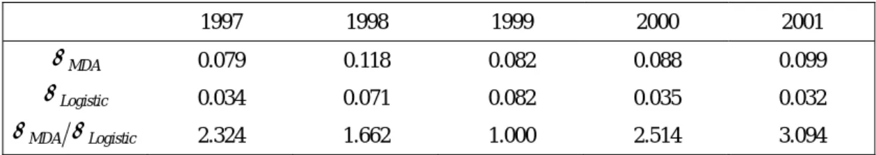
(13) firm to substitute for an actual insolvent firm.. 4.. We set apart the degree from A to E. The term A expresses that the firm has the most stable degree, B expresses the firm of a more stable degree, C+ is stable, C- is less stable, D is poorly stable (dangerous), and E expresses that the firm is insolvent.. In Table 9, we compare MDA with the logistic model for efficiency. We find that the logistic mode is more efficient than the MDA model. Therefore, we adopt the results by the logistic model. Some authors show that the MDA model is inconsistent and inefficient (Ohlson, 1980; Maddala, 1983; Barniv and McDonald, 1992) and we also achieve a similar result. Table 9 Model efficiency 1997. 1998. 1999. 2000. 2001. σ MDA. 0.079. 0.118. 0.082. 0.088. 0.099. σ Logistic. 0.034. 0.071. 0.082. 0.035. 0.032. σ MDA σ Logistic. 2.324. 1.662. 1.000. 2.514. 3.094. Here the “σ” expresses the standard variance of β.. 5. Conclusions The purpose of this study is to evaluate financial ratios as well as predictors of life insurers’ insolvency. First, we employ factor analysis to reduce the variable, and we find that the accident and health business ratio, change in fixed asset ratio, change in liquid asset ratio, and change in loan ratio are important factors for Taiwanese life insurers’ insolvency. Thus, Taiwan’s insurance commoners should be focus on the change in the fixed asset ratio, and changes in the liquid asset ratio are always very significant at insolvency. We then employ the logistic and MDA model to estimate the probability of insolvency, and the variable is the factor scores in the current year. By the logistic model, the firm’s average probability of insolvency is 10.30% from 1997 to 2001. A pessimistic conclusion is achieved by MDA, and the average probability of insolvency is 10.6%.. - 13 第五屆全國實證經濟學論文研討會 The 5th Annual Conference of Taiwan's Economic Empirics.

(14) Reference 1.. Altman. E. I. 1968. “ Financial Ratios, Discriminant Analysis and the Prediction of Corporate Bankrupt.” Journal of Finance, 23(4): 589-609. 2. Ambrose, J. M., and J.A. Seward. 1988. “ Best’s Financial Ratings, Financial Ratios and Prior Probabilities in Insolvency Prediction.” Journal of Risk and Insurance, 55:229-244. 3. Ambrose J. M. and A. M. Carroll. 1994. “ Using Best’s Ratings in Life Insurer Insolvency Prediction.” Journal of Risk and Insurance, 61:317-327. 4. Barniv, R. and M. L. Smith. 1987. “Underwriting, Investment and Solvency.” Journal of Insurance Regulation, 5: 409-428. 5. Barniv, R. 1990. “Accounting Procedures, Market Data, Cash-Flow Figures, and Insolvency Classification: The Case of the Insurance Industry.” Accounting Review, 65:578-604. 6. Barniv, R. and R. A. Hershbarger. 1990. “ Classifying Financial Distress in the Life Insurance Industry.” Journal of Risk and Insurance, 57:110-136. 7. Barniv, R. and J. B. McDonald. 1992. “ Identifying Financial Distress in the Insurance Industry: A Synthesis of Methodological and Empirical Issues.” Journal of Risk and Insurance, 59:543-574. 8. Barrese, J. 1990. “ Assessing the Financial Condition of Insurers.” CPCU Journal, 43:37-46. 9. Belth, J. M. 1984. “ Thinking the Unthinkable – What Would Happen if a Big Life Insurance Company Were to Get Into Financial Difficulty?” The Insurance Forum, 11: 29-31. 10. Breslin, C. L. and T. E. Troxel. 1978. “Property-Liability Insurance Accounting and Finance.” American Institute foe Property and Liability Underwriters. 11. Carson, J. M. and R. E. Hoyt. 1995. “ Life Insurer Financial Distress: Classification Models and Empirical Evidence.” Journal of Risk and Insurance, 62: 764-775. 12. Carson, J. M. and Scott, W. L. 1996. “ The Run on the Bank Exposure: Evidence and Implications for Life Insurer Insolvency.” The Journal of Insurance Issues, spring: 39-52. 13. Chen Y. C. and C. H. Tsai. 2002. “Capital Structure and Risk of Life insurance Companies.” Insurance Monograph, 18(1): 75-92. 14. Cheong, I. And H. D. Skipper. 1988. “A Multivariate Statistical Approach to Life Insurer Insolvency Prediction.” Research Scheme Presented at the ARIA Meeting, August. - 14 第五屆全國實證經濟學論文研討會 The 5th Annual Conference of Taiwan's Economic Empirics.

(15) 15.. Cummins. J. D., S. E. Harrington, and R. Klein. 1995. “ Insolvency Experience, Risk-Based Capital, and Prompt Corrective Action in Property-Liability Insurance.” Journal of Banking and Finance 19: 511-527. 16. Cummins. J. D., M. F. Grace, and R. D. Phillips. 1999. “ Regulatory Solvency Prediction in Property-Liability Insurance: Risk-Based Capital, Audit Ratios, and Cash Flow Simulation.” Journal of Risk and Insurance, 66(3): 417-458. 17. DeHeuck, G. T. 1981. “Is Your Company Going to be a Survivor.” Best’s Review-Life / Health Edition, 82: 20-30. 18. Gold, M. 1979. “Evaluating Life Insurance Company Performance.” Best’s Review Life/ Health Edition, 79:20-24. 19. Grace, M. F., S. E. Harrington, and R. W. Klein. 1998. “ Risk-Based Capital and Solvency Screening in Property-Liability Insurance: Hypotheses and Empirical Tests.” Journal of Risk and Insurance, 65(2): 213-243. 20. Grace, M. F., and S. E. Harrington. 1998. “Identifying Troubled Life Insurers.” Journal of Insurance Regulation, 16: 249-290. 21. Granger, G. L., J. W. Mason and S. Garrison, 1987. “ Life Insurance Company Liquidation, A Decomposition Analysis.” A Paper Presented at the ARIA Meeting, August. 22. Harmelink, P. 1974. “ Prediction of Best’s General Policyholders’ Rating.” Journal of Risk and Insurance, 41: 621-632. 23. Harrington S. E., and J. M. Nelson. 1986. “ A Regression-Based Methodology for Solvency Surveillance in the Property Liability Insurance Industry.” Journal of Risk and Insurance, 53: 583-605. 24. Huang, Chin-Sheng, Dorsey, E. Rober and A. B. Mary. 1995. “Life Insurer Financial Distress Prediction: A Neural Network Model.” Journal of Insurance Regulation, 13(2): 131-167. 25. Hershbarger, R. A. and R. K. Miller. 1986. “The NAIC Information System and the Use of Economic Indicators in Predicting Insolvencies.” The Journal of Insurance Issue and Practices, 9: 21-43. 26. Kao T. C. and S. H. Chan. 2001. “Confidence Intervals for the Probability of Insolvency in the Life Insurance Industry.” Insurance Monograph, 63: 101-121. 27. Kaiser, H. F. 1960. “ The Application of Electronic Computers Factor Analysis.” Educational and Psychological Measurement, 20: 141-151. 28. Lin S. L. 1996. “ Financial Distress Classification in the Life Insurance Industry.” Journal of Insurance Regulation, 14(3): 314-342. 29. Maddala, G. S. 1983. “Limited Dependent and Qualitative Variables in Econometrics.” Cambridge University Press. 30. Ohlson, J. A. 1980. “Financial Ratios and the Probabilistic Prediction of - 15 第五屆全國實證經濟學論文研討會 The 5th Annual Conference of Taiwan's Economic Empirics.

(16) Bankrupt.” Journal of Accounting Research, 18:109-131. 31. Pinches G. E., and Trieschmann J. J. 1974. “The Efficiency of Alternative Models foe Solvency Surveillance in the Insurance Industry.” Journal of Risk and Insurance, 41: 563-577. 32. Pottier, S. W. and D. W. Sommer. 1997. “Agency Theory and Life Insurer Ownship Structure.” Journal of Risk and Insurance, 65: 529-543. 33. Pottier, S. W. 1998. “ Life Insurer Financial Distress, Best’s Ratings and Financial Ratios.” Journal of Risk and Insurance, 65(2): 275-288. 34. Radcliffe, S. 1982. “Where Have All the Margins Gone.” Best’s Review Life / Health Edition, 82: 10-15. 35. Shaked, I. 1985. “Measuring Prospective Probabilities of Insolvency: An Application to the Life Insurance Industry.” Journal of Risk and Insurance, 52: 59-80. 36. Shiu W. Y. and E. Wang. 2003. “A Study of Minimum Capital Requirement and Capital Structure for Property-Liability Insurance Industry in Taiwan.” Journal of Risk Management, 5(1): 109-125. 37. Thornton, J. H. and J. W. Meador. 1997. “Comments on the Validity of NAIC Early Warning System for Predicting Failures Among P-L Insurance Companies.” CPCU Annals, 30: 191-211. 38. Trieschmann J. S., and G. E. Pinches. 1973. “ A Multivariate Model for Predicting Financially Distressed P-L Insurers.” Journal of Risk and Insurance, 40: 327-338. 39. Zmijewskim, M. 1984. “Methodological Issue Related to the Estimation of Financial Distress Prediction Models.” Journal of Accounting Research, 22: 59-22.. Appendix Taiwanese Life Insurance Companies, Number, and Rating in this Study. NO.. Firm’s Name. Logistic Rating. NO.. Firm’s Name. Logistic Rating. 1. CTC. C+. 16. Allianz President. C+. 2. Taiwan Life. C+. 17. ING-Aetna Life. C+. C+. 18. Georgia. C+. Prudential Life 3. Assurance 4. Cathay Life. C+. 19. Metropolitan. C-. 5. China Life. C+. 20. Prudential Life. C-. 6. Nan Shan Life. C-. 21. Connecticut General. D. 7. Kuo Hua Life. D. 22. American Life. C+. 8. Shin Kong Life. C+. 23. The Manufacturers. C-. 9. Fubon Life. B. 24. Transamerica Occidental. C-. - 16 第五屆全國實證經濟學論文研討會 The 5th Annual Conference of Taiwan's Economic Empirics.

(17) 10. Global Life Mass Mutual. 11. C+. 25. New York. C+. C-. 26. Winterthur. C+. C+. 27. Mercuries 12. Sinon. The National Mutual Life. C-. Association of Australasian 13. Singfor. C+. 28. Aegon Levensverzekering. C+. 14. Far Glory Life. C-. 29. Zurich. B. 15. Hontai Life. E. - 17 第五屆全國實證經濟學論文研討會 The 5th Annual Conference of Taiwan's Economic Empirics.

(18)