Integral Representations and Regularizations for a Divergent Series Solution of a Beam Subjected to Support Motions

Please cite this paper as follows:

Jeng-Tzong

Chen, Hong-Ki Hong, Chau-Shioung Yeh,

and S.W. Chyuan,

Integral Representations

and Regularizations for a Divergent Series Solution of a Beam Subjected to Support Motions

,

EARTHQUAKE ENGINEERING AND STRUCTURAL DYNAMICS, VOL. 25, 909-925 ( 1996)

INTEGRAL REPRESENTATIONS AND REGULARIZATIONS FOR A

DIVERGENT SERIES SOLUTION OF A BEAM SUBJECTED TO

SUPPORT MOTIONS

J. T. CHEN

Department of Harbor and River Engineering, Ocean University, Keelung, Taiwan

H.-K. HONG

Department of Civil Engineering, Taiwan Universi1.y. Taipei, Taiwan

C. S. YEH

National Center for Research on Earthquake Engineering, Taipei, Taiwan

AND S. W. CHYUAN

Chung-Shan Insiitute of Science and Technology, Lungtan. Taiwan

SUMMARY

Derived herein is the integral representation solution of a Rayleigh-damped Bernoulli-Euler beam subjected to multi-support motion, which is free from calculation of a quasi-static solution, and in which the modal participation factor for support motion is formulated as a boundary modal reaction, thus making efficient calculation feasible. Three analytical methods, including ( 1 ) the quasi-static decomposition method, (2) the integral representation with the Cesaro sum technique, and (3) the integral representation in conjunction with Stokes’ transformation, are presented. Two additional numerical methods of (4) the large mass FEM simulation technique and (5) large stiffness FEM simulation technique are easily incorporated into a commercial program to solve the problem. It is found that the results obtained by using these five methods are in good agreement, and that both the Cesiro sum and Stokes’ transformation regularization techniques can extract the finite part of the divergent series of the integral representation. In comparison with the Mindlin method and Cesaro sum technique, Stokes’ transformation is the best way because it is not only free of calculation of the quasi-static solution, but also because it can obtain the convergence rate as rapidly as the mode acceleration method can.

KEY WORDS : regularization; divergent series; support motions; Stokes’ transformation; Cesiiro sum; bridge

1. INTRODUCTION

Since Loh’ used SMART-1 data, which were obtained in 1982 from a seismograph array in Lotung, Taiwan, to analyse the effect of spatial variation of ground motion on structural responses, several investigators have studied the problem of multi-support excitation to identify the need of such analysis. In fact, multi-support vibration happens frequently, e.g. seismic responses of pipelines and long bridges whose abutments and piers are far apart so that the surrounding topography and geology may be different as schematically shown in Figure 1. Most attention has been paid to the analysis of these systems to obtain design forces during an extreme event induced by earthquake ground motion. Following the paper of Mindlin and Goodman: these problems have all, to our knowledge, been solved by decomposing the solution into two parts artificially. Clough and Penzien3 applied the Mindlin4oodman method to the discrete system of a finite element formulation and found that the computational effort for the quasi-static solution was very large. Masri4 used the same method

CCC 0098-8847/96/090909-17

@

1996 by John Wiley & Sons, Ltd.

Received I0 January 1995

Figure 1 . A long bridge subjected to seismic ground motion

to examine the response of a beam to propagating boundary excitation and considered random excitation of a shear beam in his paper.' In 1982, Abdel-Ghaffar and Rood6 applied the same method to the analysis of a tower of the Golden Gate Bridge.

Although Mindlin and Goodman2 proposed a quasi-static decomposition method for problems with time- dependent boundary conditions, Eringen and Suhubi7 found that obtaining a quasi-static solution is still a difficult task. They omitted calculation of the quasi-static solution and merged it into the total solution after considering Betti's law between the eigensystem and the quasi-static solution. This procedure reduced the solution to that of eigenfunction expansion. Although it is good to eliminate calculation of the quasi-static solution, a low convergence rate due to the Gibbs phenomenon8y9 for the primary field and divergence for the secondary field have been noted by Strenkowski. lo Nevertheless, the regularization for divergent series

has not been dealt with previously due to the problem created by omitting the calculation of the quasi-static solution.

In the present paper, we combine the concept of dual integral representation"Yi2 with either the Cesaro sum t e ~ h n i q u e ' ~ . ' ~ or Stokes' transformati~n,'~ and apply the idea of Eringen and Suhubi to solve the problem of a long bridge subjected to multi-support motions. Finally, two numerical methods including large mass and large stiffness techniques are employed for comparison with the three analytical solutions.

2. ANALYTICAL FORMULATION FOR A RAYLEIGH-DAMPED BERNOULLI-EULER BEAM SUBJECTED TO SUPPORT MOTIONS

The seismic response of a Rayleigh-damped Bernoulli-Euler beam subjected to multi-support excitation shown in Figure 2 can be described by the following governing equation:

a4u(x, t )

pAii(x,t)+

(

@,r)+EZ- = f ( x , t ) , 0 < x

<

1

ax4

where a superimposed dot denotes a time derivative, E l , @ and I denote the flexural rigidity, mass per unit length and length of the single-span beam of the bridge, respectively, a and

p

are coefficients of the Rayleigh damping, and u is the displacement, which is a function of position x and time t. For simplicity, but without

A BEAM SUBJECTED TO SUPPORT MOTIONS 91 1

red system

quasi-static system

elgeksystem e/gen-system

+

p

-q

KCtl

+

0 0 q1 ft)

q p

0 a Q"(t1

+

elgenf unctlon expanslon

n

M

)

t

quasi-static decomposition

aft)

f

lnal

behavlor

Figure 2. A simple model for a beam subjected to multi-support motions

loss of generality, the load f ( x , t ) is assumed to be zero during an earthquake. The boundary conditions are

u(0, t ) = a ( t ) , u ( l , t ) = b ( t ) ( 2 )

(3

1

where a superscript prime stands for a spatial differentiation, and a ( t ) and b(t) are support motions prescribed

by records of ground motion. In the numerical examples, the inphase and outphase motions for a ( t ) and b ( t ) will be considered.

u"(0, t ) = u"(

I,

t ) = 0

Assuming that the motion starts from rest, the initial conditions are

u(x,O) = 0, li(X,O) = 0. (4)

2.1. Quasi-static decomposition method

As shown in Figure 2, the solution can be decomposed into two parts:

oc

u(x, t ) = W X , t )

+

c

qn(t)un(x)

n=l

where U ( x , t ) denotes the quasi-static solution, and the natural modes u,(x) weighted by generalized co- ordinates qn(t) are the dynamic contribution due to the inertia effect. The quasi-static part U ( x , t ) must satis@

= o

a 4

u(x,

t

and is subject to non-homogeneous boundary conditions:

U ( 0 , t ) = a ( t ) , U(Z,t) = b ( t ) U ” ( 0 , t ) = U”(1,t) = 0

By solving the PDE in equation (6) with boundary conditions in equations (7) and (8) directly, we have

X

U k t ) = a ( t ) (1 -

-)

1

+

b ( t )

(5)

(9)

The nth natural mode u,(x) with frequency w, of the eigen-system is

u,(x) = sin ( n n x / l ) , n = 1,2,.

. .

(10)

and the corresponding natural fiequencies are

w, =

(nn/l)2dG&Zj,

n = 1,2

...

The orthogonality conditions of the eigenhctions are

pu,(x)uk(x) dx = &N, n,

k

= 1,2..

.

I’

where N

=

p1/2. Substituting (5) into (l), we obtain

n= 1

where the nth damping ratio

5,

is defined by

25,w, ZE 2a

+

pw,Z (14)

Multiplying both sides of (13) by u&), integrating over ( 0 , l ) and applying the orthogonality conditions of

(12), we have q n ( t ) satisfying the following relation:

where

F,(t) E -

1’

p U ( x , t ) u , ( x ) dx

After considering the initial conditions, we have

N 4 , ( 0 ) =

-

1’

pir(x,O)u,(x) dx =

P,(O).

(18)

It is observed that if U ( x , t ) is known, q n ( t ) can be determined by equations (15), (17) and (18), and then the series solution of equation ( 5 ) can be obtained.

Here, we apply a technique to calculate Fn(t) without first determining U ( x , t ) ; thus, the domain integration of equation (16) is avoided. Now, choosing the quasi-static solution and the eigen-system as two systems, Betti’s reciprocal relation or Green’s formulaI6 yields

A BEAM SUBJECTED TO SUPPORT MOTIONS 913

where R: and Rf, are the modal reaction forces of the nth mode at x = 0 and x = 1, respectively. Equation ( 1 9 ) is remarkable in that the integration over the domain, 0 to 1, is transformed to boundary data on x = 0 and 1. By the definition of equation ( 1 6 ) , ( 1 9 ) can be rewritten as

w;Ffl(t) = R: a ( t )

+

RI, b ( t ) ( 2 0 ) Thus, we can solve for q f l ( t ) by using equations (15), ( 1 7 ) and ( 1 8 ) , that is

sin (w:t)

+

q [ e - t n m n l sin ( w i t ) ]

tfl

Jm

1

qfl(t) = qfl(0)e-t~mJ

x [ R : a ( r )

+

Rib(?)

+

2a(R:u(r)

+

RAd(z))] d.r

where w: f

w n d R

is the nth damped frequency. Eq.(21) can be rewritten in another form:

x [ R $ z ( z ) + R i b ( ? )

+

/?(R:li(z)

+

RAd(t))] dz ( 2 2 ) Then, the series solutions for displacement u, slope 0, moment A4 and shear force V can be expressed, respectively, as

r M

cos

(7)

I

--

n2 a2

M ( x , t ) = EZu”(x, t ) = EZ U”(x, t )

I

+

qfl(t)

(

7

sin

(7

)

)]

fl=l

M

V ( x , t ) = EZu“‘(x, t ) = EZ

qfl(t)

($)

cos

(7

)]

where qfl(t) can be replaced by either equation ( 2 1 ) or (22).

In deriving equations (24 ) - ( 2 6 ) , the termwise differentiations of equation ( 2 3 ) are permissible due to good matching of prescribed data on the boundary. However, this is not permissible in the method described in the following subsection since it renders unmatched boundary data.

2.2. Eigenfunction expansion method

From equations ( 1 2 ) and (16), the Fourier series representation for U ( x , t ) is found as follows:

00

U ( X , f ) = -

c

Fm(f)u,(x)

N

m= I

If a more generalized coordinate, q f l ( t ) , is defined as

then the solution of u is available upon substituting equations (lo), (22) and (30) into (5) and using (20):

x [R:a(z) + R i b ( ? )

+

/3(R:u(z)

+

Rid(z))] dz sin ( n m / l )

I

(29)

The displacement response in equation (29) has been formulated as an integral representation solution which contains both the Duhamel integral in time and the boundary integral in space; in this case, only two boundary modal data are concerned due to the one dimensional domain. Therefore, the above equation reveals a new point of view that the modal participation factors for support motions u ( t ) and b (t ) are simply -R:/N and -R!,/N, respectively, under the condition of

/3

= 0.

Without thoughtll consideration, term by term differentiations of (29) yield

x[R:u(z> + R i b ( ? )

+

/3(R:u(z)

+

R i d ( z ) ) ] dz

I

(

y )

cos

(

y )

- n 3 z 3

x [ R z a ( z )

+

Rib(z)

+

/3(R:u(z)

+

R;d(z))] dz]

( -7i-)

cos

( y )

In addition to the troublesome equation (29), the three expressions (30)-(32) are worse. Because the support motion acts as a double layer potential, which is the terminology of potential theory and the dual integral representation,’ ‘ 9 12, the series for displacement is pointwise convergent in the sense that the discontinuity

across the boundary can be described by a series representation. Therefore, the term by term differentiations of the series for displacement to determine slope, moment and shear force will result in a divergent series.

An appropriate regularization technique is necessary to extract the finite part; for the series forms of equations

(29)-(32) in this paper, we shall employ the Ceshro sum regularization technique, which plays the same role as does the regularization method for the derivative of the double layer potential.

2.3. Regularization with Cesdro sum technique The general ( C , r ) Ceshro s u m is defined asI4

A BEAM SUBJECTED TO SUPPORT MOTIONS 9 1 5

where C,“ = k ! / ( r !

(k

- r ) ! ) , and the partial sum is

k k

sk = q n ( t ) U n ( x ) =

c

an(x, t ) (34)

n=O n=O

For efficiency of computation, the si terms are changed to ai terms, and the equation is, thus, changed to the conventional Cesiro sum:

Similarly, the (C, 2 ) , (C, 3 ) and (C, 4) Cesaro sum is

(37)

Based on this regularization technique, the series representations for displacement, slope, moment and shear force are expressed in the sense of the Cesaro sum as follows:

The Gibbs phenomenon exhibited in the pointwise convergent series of equation (29) can be avoided by using the CesPro regularization technique, and the finite part of the divergent series in equations (30H32) can be extracted as shown in (41H43).

2.4. Regularization with Stokes' transformation

Although termwise differentiations are not permissible for the pointwise convergent series representation for

u ( x , t ) in the classical sense, the differential operator can still be applied directly as in equations (30H32) of Subsection 2.2, and then the posterior treatment of the CesAro sum can be used to ensure the sumability as in Subsection 2.3. Here, we introduce a logical way of differentiating the pointwise convergent series, which is called Stokes' tran~formation,'~ and use the unmatched boundary data as shown below.

Consider the displacement function u(x, t ) represented by a Fourier sine series in the open interval 0 < x

<

1

with the given histories a ( t ) and b ( t ) at the end points:

x = o

Assume

multiplying both sides of the above expression by c o s ( n m / l ) and integrating over ( O , l ) , and considering equation

(44),

we have & ( t ) = and Defining rn we have 2 - [ ( - l ) " b ( t ) - a ( t ) ] + n x c & ( t ) / l , n = l,2,

...

1 - 1 1 & ( t ) = - [ a ( t )

-

b ( t ) ] , for n = 0 & ( t ) = r n ( t )

+

nmjfl(t)/l, n 2 O (46) (47) (49)

It is easily found that direct term by term differentiation of the Fourier sine series in equation (44) loses the r,, terms, which can be recovered by Stokes' transformation as shown above or by the posterior regularization treatment of the Cesaro sum method as described in the previous subsection.

In order to improve the rate of convergence for u(x,t) at the points near the boundary as x approaches 0 or 1, u(x,t) can be calculated by integrating (45) from 0 to x:

A BEAM SUBJECTED TO SUPPORT MOTIONS 917

Comparing equation (50) with (44), the additional three terms result in improvement in the convergence rate. Similarly, applying the Stokes’ transformation again, the moment and shear force can be expressed as follows:

where

q;(t) = --nn&(t)/l, n = 0,1,2,. .

.

(53) (54) q y ( t ) = -n 2 n 2 - 1 q , ( t ) / P , n = 0 , 1 , 2 . .

.

It is found that the solution also contains two parts, modal and non-modal parts. However, the solution of the non-modal part results from the integration of the secondary field solution in a way different from using the quasi-static decomposition method which derives the non-modal part by solving the P.D.E. directly. No doubt, the Stokes’ transformation is easier.

(a)

Large

mass

model

(b)

large

stiffness model

2.5. Large mass simulation technique

In this and the next subsections, alternative numerical methods will be explored. In order to satisfy the boundary support motion histories, the large mass technique is used here and incorporated into MSCNAST

RAN. At the left end, x = 0, a large mass

4

is mounted. A should be much larger than A,, which denotes the total structural mass. Likewise, at the other end, x = I , the large mass A is also assumed. Thus, the external agency exerts the forces of .Mu(t) and A & ( t ) at the two ends of the free-free beam, respectively, to ensure the enforced acceleration histories u ( t ) and & ( t ) as shown in Figure 3(a).

2.6. Large stiffness simulation technique

Instead of using the large mass simulation technique, the large stiffness simulation can also describe the equivalent system. At x = 0, a spring with large stiffness X is introduced. X should be much larger than

X , , which denotes the structural stiffness. In the same way, a spring with large stiffness X is also assumed at x = 1. Both springs are connected to the ground. The external agency exerts the forces X a ( t ) and X b ( t ) at the two ends, respectively, to ensure the enforced displacement histories a ( t ) and b ( t ) for the constrained motion as shown in Figure 3(b).

3. ILLUSTRATIVE EXAMPLES

In order to see the validity of the three analytical solutions and the two finite element simulation techniques for the multi-support seismic response, examples will be furnished and comparisons made between the three analytical solutions and finite element outputs using two simulation techniques.

The input data are as follows: 1 = 60 m,

EZ

= 2.45 x lo9 Nm2, p A = 2400 kgm-', a ( t ) = SO e-61 sin ( a t ) H ( t ) and b ( t ) = H(t - td)a(t - t d ) , SO = 0.01 m, 6 = 0.1, where H ( t ) is the Heaviside function, td is the time lag, 6 is the decaying rate of the support motion, So is the magnitude and R is the excitation frequency for all of the support motions.

Case 1: A damped ( a = 0.138 1 s-l,

p

= 0 s) Bernoulli-Euler beam subjected to in-phase multi-support excitations:

Case 2: A damped ( a = 0.138 1 s-l,

p

= 0 s) Bernoulli-Euler beam subjected to out-of-phase multi- support excitations:

Case 3: A Rayleigh-damped ( a = 0.11 1 1 s-l,

p

= 0.0072 s) Bernoulli-Euler beam subjected to in-phase multi-support excitations:

3.1. Quasi-static decomposition method (method ( 1 ) )

solution:

Substitution of modal reactions for R,(O) and R n ( l ) into equation (23) yields the explicit form of the

where

'+'

and '-' represent the in-phase and out-of-phase motions, respectively, and +L(t) can be easily determined as in Reference 12. The displacement histories at x = 15, 30m for case 1 and x = 15 m for case

A BEAM SUBJECTED TO SUPPORT MOTIONS 0.03 919

-

quasi-static decomposition Cesaro sum Stokes' transformation

---.

'

-

t

-0.03 0 2 4 6 a 10 -0.04

'

' time (sec)

Figure 4. The solutions of in-phase motions at x = 15 or 45 rn using methods (1 H5) with five modes and 25 elements

0.04 0.03 0.02 4 0.01 E: E v e, 8 0

1

;ii

-

_a -0.01 -0.02 displacement history at x=30 m

-

quasi-static decomposition Cesaro sum Stokes' transformation

-

-

large mass simulation

V

t

-0.03 0 2 4 6 a 11 -0.04 t , time (sec)

Figure 5. The solutions of in-phase motions at x = 30 using methods ( 1 H5) with five modes and 25 elements

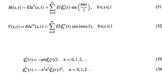
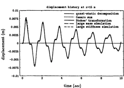
2 are shown in Figures 4, 5 and 6 , respectively. The displacement, slope, moment and shear force diagrams at t = 1 s for cases 1 and 3 are shown in Figures 7-10, respectively.

3.2. Eigenfunction expansion method

Substitution of modal reactions for R,(O) and

R,(Z)

into Eq.(29) yields the general solution

where

'+'

and '-' denote the out-of-phase and the in-phase motions, respectively, and & ( t ) can be easily determined as in Reference 12. Since the Gibbs phenomenon in the displacement response and the divergent solutions in the slope, moment and shear force occur, the following two regularization techniques are employed to extract the finite values.

h

E

v dimplaceanant history a t x=15 m 0 .Ol 0.0075 Cesuo sum Stokes' transformation

--

l u g e mass simulation 0.005

---

l u g e stiffness simulation h Ej

5

B

-

0.0025 0

.!

-0.0025 -0.005 -0.0075 ' -0.01. Y

B

V 0 2 4 6 8 10 ' time (scc)

Figure 6. The solutions of out-of-phase motions at x = I5 using methods ( 1 ) 4 5 ) with five modes and 25 elements

I 1

0.015

---Cesaro Bum

-Stokes' transformation

0 10 20 30 40 50 60

dirplacament diagram at t=l sac -quasi-static decampasition ---Cesaro sum

_-...---..

0.0005 I I 0 10 20 30 40 50 60 h E !? Y al 2 8

?

4

-100000 -120000 -140000 0 10 20 30 40 50 60

moment diagram a t t=l sec

2000

0 10' 20 30 40 50 60

slope diagram a t t-1 sec _{ahear diagram a t t i 1 sec}

Figure 7. The series solutions for the displacement, slope, moment and shear force at r = 1 s using methods (1 )43) with five modes for case 2 when damping is proportional to mass only

3.3. Regularization with the Cesaro sum (method ( 2 ) )

Using equations (40)-(43), the numerical results of the displacement, slope, moment and shear force re- sponses can be easily calculated as shown in Figures 7-10 for cases 1 and 3. The displacement histories at

A BEAM SUBJECTED TO SUPPORT MOTIONS 92 1 0 - -20000 -40000 -60000 -80000 Y

s

-Stokes’ tranrformation

.-

a ’ -0.005

1

1 0 10 20 30 40 50 60 -120000 q u a s i - s t a t i c docomposit ’ -loo000 -80000

1

-

4

P

I

-12Oooo ’ -140000 -160000 I 10 20 30 40 50 60

0

displacement diagram at t=l sec m o m a n t diagram a t t=l sec

----cesaro sun

0 10 20 50 40 50 60 -60000 0 10 20 30 40 50 6

shear diagram a t ti1 sec slops diagram a t t-1 sec

Figure 8. The series solutions for the displacement, slope, moment and shear force at t = 1 s using methods (1x3) with one hundred modes for case 2 when damping is proportional to mass only

0.015 . -Stokes’ transformation 0 10 20 30 40 SO 60 h

E

I . I 0 10 20 30 40 50 60

displacemant diagram a t t=l sec moment diagram a t t=l roc -quasi-static decomporition ---Cesaro sun

i

0.0005 h

2

v

!

-0 .ow5 -0.001

.

...___._.

-.----

\I

I I 0 10 20 30 40 50 60 .--4. 8000, I -quasi-static decompoait\ph ---Cesaro sun 4000

6ooo

I

-Stokes’ transformatioq,,,’

2000

\

0 10 20 30 40 50 60

-8000

shear diagram a t ti1 sec

slop. diagram a t t=l sec

Figure 9. The series solutions for the displacement, slope, moment and shear force at t = 1 s using methods (1 H3) with five modes for case 3

0.015 ’ ---Ceaaro m a --Stoker’ transformation 0 10 20 30 40 50 60

-

_E

0

5

I

-100000 -120000 -140000 0 10 20 30 40 50 SO

dimplacement diagram at t=l aec moment diagram at t=l aec

10 20 30 40 50 60

alope diagram at t=l aoc shear diagram a t t-1 aec

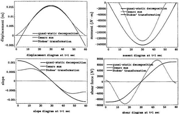
Figure 10. The series solutions for the displacement, slope, moment and shear force at t = 1 s using methods ( 1 H 3 ) with 100 modes and method (5) using 25 elements for case 3

3.4. Regularization with Stokes’ transformation (method ( 3 ) )

Substituting the same values as in Subsection 3.2 for 4 J t ) of equations (50), (45), (51) and (52), the numerical results of the displacement, slope, moment and shear force responses can be easily calculated and are shown in Figures 7 and 8 for case 1 and in Figures 9 and 10 for case 3.

3.5. Large mass simulation technique (method ( 4 ) )

Twenty-five CBAR beam elements and 500 time step intervals are used. The large mass ratio is suggested as being lo6 in this case. Note that in addition to the original modes, two very low frequency modes due

to the two large masses should be included in the modal superposition in order to simulate the enforced boundary support acceleration. The input data can be prepared easily’9 for the program and is omitted here. For the interior points x = 15, 30m for case 1 and at x = 15 m for case 2, the displacement histories are in good agreement with analytical solutions as shown in Figures 4-6, respectively.

3.6. Large stifness simulation technique (method ( 5 ) )

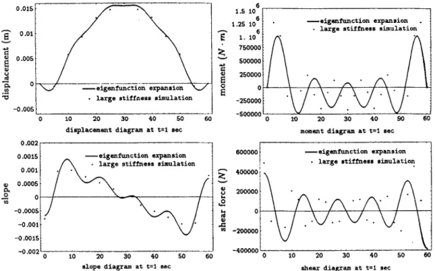
The same mesh configuration and time steps as in Subsection 3.5 are used. The large stiffness ratio is suggested as being lo6 in this case. In comparison with the original modes, two additional very high frequency modes for the deformation of the two large springs should be included in the modal superposition in order to simulate the enforced boundary support displacement accurately. If the two largest modes are truncated in modal analysis, the boundary displacement will not match the enforced displacement, while the slope, moment and shear force distributions will diverge in a way similar to that in the eigenfunction expansion method as shown in Figure 11. When the two modes are included, the boundary displacement and slope solutions from FEM approximate the analytical solutions, but the boundary layer effect is still obvious for the moment and shear force distributions as shown in Figure 10. For the interior points x = 15, 30m for case 1 and at

A BEAM SUBJECTED TO SUPPORT MOTIONS 923 1.5 10 1.25 10 6 0.015 ’ . - -

__

-eigenfunction expansion W

.

large stiffness simulation

-eigenfunction expansion

.

*

0.015

large stiffness simulation

-0.005

1

0 10 20 30 40 50 60

displacement diagram at t=l sec m o m e n t diagram a t t=l sec 0.002

600000 -eigenfunction expansion

-eigenfunction expansion

.

large stiffness simulation

.

large stiffness simulation

-0.0015

-0.002

0 10 20 30 40 50 60

slope diagram at t=l sec shear diagram at t-1 sec

Figure 1 1 . The series solutions for the displacement, slope, moment and shear force at t = 1 s using the eigenfunction expansion method and large stiffness simulation without considering the two largest modes using 10 modes for case 3

x = 15 m for case 2, the displacement histories are in good agreement with analytical solutions as shown in

Figures 4-6, respectively.

4. COMPARISONS AND DISCUSSIONS

The displacement histories at x = 15, 30m for case 1 and at x = 15 m for case 2 are depicted in Figures 4-6

using five modes and 25 elements. It can be seen that the results of all five methods are in good agreement. The displacement, slope, moment and shear force diagrams of case 1 at t = 1 s using methods (1)-(3) are shown in Figures 7 and 8 for mode number = 5 and 100, respectively. Unfortunately, the shear force result diverges as shown in Figure 8. For case 3, the displacement, slope, moment and shear force diagrams at t = 1 s using methods ( 1 H 3 ) are shown in Figures 9 and 10 for mode number = 5 and 100, respectively.

Although the shear force response is divergent for case 1 in Figure 8, it is convergent for case 3 using the

three analytical formulations as shown in Figures 9 and 10, respectively. This motivates us to analyse the asymptotic behaviours of q,,(t) and q,,(t) as the mode number becomes infinite. It is found that the solution of displacement in case 2 is governed by O(l/n3) of the q,, terms, as

5,

-+ O(l/n2) for p = O . The asymptotic

behavior of the displacement, u ( x , t ) , in case 3 is governed by O(l/n5) of the s,, terms, as

5,

+ O ( n 2 ) for

p

#

0. In deriving the series solution of the shear force, three-fold differentiation with respect to x causes the solution to have O(1) asymptotic behavior after an additional O ( n 3 ) multiplication. This is the reason why the shear force response of case 2 is divergent. Extending this concept to acceleration, the results for case 2

are also divergent. To summarize:

1. It must be noted that the general solutions of methods ( l ) , (2) and (3) are formulated as boundary

integrals or data instead of domain integration. Therefore, a new point of view regarding the modal par- ticipation factor has been developed. Recently, two applications of this concept have been successhlly applied.”.’

2. The convergent solution can only be used to obtain the displacement, slope and moment, not the shear force response when damping is proportional to mass only as shown in Figure 9 for case 2. The results can be understood from the order analysis of the solution. It can be seen that the shear force results are not available for the same example in Reference

4.

3. For the large stiffness simulation, the inclusion of the two additional high frequency modes enables matching of the boundary support displacements. The two additional modes can be easily found from the obtained modes by FEM(NASTRAN in this paper) since the deformation for the two high-frequency modes locally concentrates on the spring instead of the beam. If the contribution of the two modes is neglected, the results diverge in the same way as with the eigenfunction expansion method as shown in Figure 11. Even if the two modes are considered, the boundary layer effect is present in the moment and shear force responses as shown in Figure 10. To explain this phenomenon, the free body diagram in Figure 3 reveals that the simulation model cannot simulate the end shear equivalently, i.e. inconsistency exists between the original problem and the proposed simulation model. By the same token, the large mass simulation has a similar boundary layer effect.

5 . CONCLUSIONS

The analytical solutions of a Rayleigh-damped Bernoulli-Euler beam subjected to multi-support motions have been derived by means of three different analytical formulations and compared with two numerical methods in this paper. The results obtained using the five methods are in good agreement.

Mindlin and Goodman solutions behave well at the expense of the additional effort involved in determination of the quasi-static solution; this effort is substantial in most real-world problems. To avoid calculation, the quasi-static solution is expanded in the Fourier series sense; or, interpreted in another way, the problem is solved directly in the eigenfunction (generalized Fourier series) expansion sense, thus rendering a pointwise convergent series solution for the displacement response, which does not converge to the prescribed support motions at the two ends and exhibits the Gibbs phenomenon near the boundary and divergent series solutions for the slope, moment and shear responses. It has been shown that the boundary layer effect and divergence can be dealt with by using the Ceshro sum technique, which smoothens the oscillating behaviour of the displacement and extracts the finite parts of the divergent series solutions. Although it is capable of recovering the finite part of the existing response without obtaining the quasi-static solution, the CesAro sum technique requires a larger number of modes in calculating the response near the boundary for the boundary layer effects described above. In order to improve numerical efficiency, the Stokes’ transformation technique is utilized to accelerate convergence since it takes advantage of prescribed data of support motions. This feature can save a large amount of computational effort and is highly recommended. An extension to real structures by using a discrete system has been successfully applied.18

After comparing the FEM results with the three analytical results, care should be taken to add boundary modes corresponding to the large masses and stiffnesses if the slope response is considered. For the moment and shear force responses, the boundary effect is apparent and more research effort on this effect is needed in the future.

ACKNOWLEDGEMENTS

C. S. Yeh gratefully acknowledges the financial support granted by the National Science Council, the R.O.C., through the National Center for Research on Earthquake Engineering (NSC 82-061 7-3-002-001).

REFERENCES

1. C. H. Loh, J. Penzien and Y. B. Tsai, ‘Engineering analysis of SMART-I array accelerograms’, Earfhquake eng. sfrucr. dyn. 10,

2. R. D. Mindlin and L. E. Goodman, ‘Beam vibrations with timedependent boundary conditions’, J. appl. mech. ASME 17, 377-380 3. R. W. Clough and J. Penzien, Dynamics of Sfrucrures, McGraw-Hill, New York, 1975.

4. S. F. Masri, ‘Response of beams to propagating boundary excitation’, Earthquake eng. sfrucf. dyn. 4, 497-509 (1976). 575-591 (1982).

A BEAM SUBJECTED TO SUPPORT MOTIONS 925

5. S. F. Masri and F. Udwadia, ‘Transient response of a shear beam to correlated random boundary excitation’, J. app. mech. ASME 6. A. M. Abdel-Ghaffar and J. D. Rood, ‘Simplified earthquake analysis of suspension bridge towers’, J. eng. mech. diu ASCE 108(2), 7. A. C. Eringen and E. S. Suhubi, Elastodynamics, Vol. 11, Linear Theory, Academic Press, New York, 1975.

8. L. Meirovitch and M. K. Kwak, ‘Convergence of classical Rayleigh-Ritz method and finite element method’, AIAA J. 28(8),

9. S. S. K. Tadikonda and H. Baruh, ‘Gibbs phenomenon in structural mechanics’, AIAA J. 29(9), 1488-1497 (1991).

44, 4 8 7 4 9 1 (1977). 291-308 (1982).

1509-1 5 16 ( 1990).

10. J. S. Strenkowski, Dynamic response of linear damped continuous structural members, Ph. D. Dissertation, Department of Mechanical 11. J. T. Chen and H.-K. Hong, Boundary Element Method, 2nd edn, New World Press, Taipei, Taiwan, 1992 (in Chinese).

12. J. T. Chen, On a dual representation model and its applications to computationai mechanics, Ph.D. Thesis, Department of Civil 13. G. M. Fichtenholz, Infinite Series: Ramifications, Gordon and Breach, New York, 1970.

14. G. H. Hardy, Divergent Series, Oxford Univ. Press, London, 1949.

15. T. J. I’anson Bromwich, An Introduction to the Theory of Infinite Series, Macmilan, London, 1965. 16. E. L. lnce, Ordinary Direrential Equations, Dover, New York, 1956.

17. H.-K. Hong and J. T. Chen, ‘Derivation of integral equations in elasticity’, J. eng. mech. diu ASCE 114(6), 1028-1044 (1988).

18. J. T. Chen, H.-K. Hong and C. S. Yeh, ‘Modal reaction method for modal participation factor of support motion problems’, Comm. 19. M. A. Gockel, Handbook of Dynamic Analysis, MacNeal-Schwendler Corp., 1983.

20. J. T. Chen and Y. S. Cheng, ‘Dual series representation for a string subjected to support motions’, Adu. Eng. Software. accepted,

21. J . T. Chen and D. H. Tsaur, ‘A new method for transient and random responses subjected to support motions’, Engineering Structures, 22. J. T. Chen et al., Finite Element Analysis and Engineering Applications using MSCNASTRAN, Northern Gate Pub]., Taipei, Taiwan,

and Aerospace Engineering, University of Virginia, 1976.

Engineering, National Taiwan University, 1994.

numer. methoh eng. 9, 4 7 9 4 9 0 (1995).

1996. accepted, 1996. 1996 (in Chinese).