An HVS-Directed neural-network-based image resolution enhancement scheme for image resizing

An HVS-Directed Neural-Network-Based Image

Resolution Enhancement Scheme for Image Resizing

Chin-Teng Lin, Fellow, IEEE, Kang-Wei Fan, Her-Chang Pu, Shih-Mao Lu, and Sheng-Fu Liang

Abstract—In this paper, a novel human visual system (HVS)-directed neural-network-based adaptive interpolation scheme for natural image is proposed. A fuzzy decision system built from the characteristics of the HVS is proposed to classify pixels of the input image into human perception nonsensitive class and sensitive class. Bilinear interpolation is used to interpolate the nonsensitive re-gions and a neural network is proposed to interpolate the sensi-tive regions along edge directions. High-resolution digital images along with supervised learning algorithms are used to automati-cally train the proposed neural network. Simulation results demon-strate that the proposed new resolution enhancement algorithm can produce a higher visual quality for the interpolated image than the conventional interpolation methods.

Index Terms—Fuzzy decision system, human visual system, image interpolation, neural network, resolution enhancement.

I. INTRODCTION

I

N recent years, consumer digital image/video capture/ display devices such as digital still cameras, digital video cameras, multiple-function peripherals, etc., have become more and more popular, such that image interpolation has become an increasingly important technology for image format/resolution conversion. Image interpolation addresses the problem of gen-erating a high-resolution image from its low-resolution image version. It is known that conventional interpolation techniques such as the bilinear and the bicubic interpolations do not satisfy the requirements since these methods tend to cause problems such as blurring and jaggedness around the edges. An ideal interpolation scheme should always go along the edge so that this area will not blur and the smoothness will be preserved.

Recently, several adaptive nonlinear methods have been pro-posed to tackle these problems. They analyze the image first to achieve better interpolation quality [1]–[4]. Much research has been done to improve the subjective quality of the interpolated

Manuscript received January 7, 2005; revised March 17, 2006. This work was supported in part by the Ministry of Economic Affairs, Taiwan, under Grant 95-EC-17-A-02-S1-032, the National Science Council, Taiwan, under Grant NSC95-2752-E-009-011-PAE, and by the MOE ATU Program under Grant 95W803E.

C.-T. Lin is with the Department of Electrical and Control Engineering and Department of Computer Science, National Chiao-Tung University (NCTU), Hsinchu 300, Taiwan, R.O.C., and with the Brain Research Center, NCTU Branch, University System of Taiwan, Hsinchu 300, Taiwan, R.O.C. (e-mail: ctlin@mail.nctu.edu.tw).

K.-W. Fan, H.-C. Pu, and S.-M. Lu are with the Department of Electrical and Control Engineering, National Chiao-Tung University, Hsinchu 300, Taiwan, R.O.C. (e-mail: cpu@mail.nctu.edu.tw).

S.-F. Liang is with the Department of Biological Science and Technology, National Chiao-Tung University, Hsinchu 300, Taiwan, R.O.C., and with the Brain Research Center, NCTU Branch, University System of Taiwan, Hsinchu 300, Taiwan, R.O.C. (e-mail: sfliang@mail2000.com.tw).

Digital Object Identifier 10.1109/TFUZZ.2006.889875

images. Adaptive interpolation schemes [6], [12], [14], [27], [28] spatially adapt the interpolation to better match the local structure around the edges. PDE-based schemes [29], [30] improve the image quality using a nonlinear diffusion process controlled by the local gradients. Edge-directed interpolation [31], [32] employs a source model emphasizing the visual integrity of detected edges and modifies the interpolation to fit into the source model. The neural-network (NN)-based scheme had also been proposed for image interpolation [15]. All of the above schemes demonstrate improved visual quality in terms of sharpened edges or suppressed artifacts. Since human eyes are more sensitive to the edge areas than the smooth areas within an image, many algorithms [5]–[15] have been proposed to improve the subjectively visual quality of edge regions in the images that need interpolation applied to them. However, how to design the optimal-adaptive filter to improve the quality of interpolated images is the challenge for these methods. It is well known that the statistics of image signals are quite nonstationary and the fidelity of the reconstructed images demanded by the human eye differs from pixel to pixel. More and more approaches have been proposed to incorporate the characteristics of the human visual system (HVS) into the digital image processing such as watermark encoder design [16]–[18], digital image compression [19], [20], and image recognition [21], [22].

In this paper, a novel HVS-directed adaptive interpolation scheme is proposed to combine the bilinear interpolation and an artificial neural network for image interpolation to balance the tradeoff of speed and quality. A fuzzy decision system [23], [24] inspired by the human visual system is proposed to clas-sify the input image into human perception nonsensitive regions and sensitive regions to select either the bilinear interpolation module or the proposed neural-network interpolation module to operate for each region. High-resolution digital images com-bined with supervised learning algorithms can be used to au-tomatically train the proposed neural network [25], [26]. Ac-cording to the experimental results, the proposed HVS-directed neural-network-based image interpolation technology is far su-perior to conventional methods in some aspects, such as the clarity and the smoothness in the edge regions as well as the visual quality of the interpolated images.

This paper is organized as follows. Section II introduces the system structure of the proposed image interpolation method, and an HVS-directed fuzzy system for image analysis is also proposed in this section. A neural-network-based image interpo-lation method is represented in Section III. Section IV presents the experimental results for demonstration. Section V concludes this paper.

Fig. 1. Schematic block diagram of the proposed image resolution enhance-ment systems.

Fig. 2. (a) A 42 4 sliding block in the original image. (b) The block after two times interpolation.

II. SYSTEMARCHITECTURE AND HVS-DIRECTED

IMAGEANALYSIS

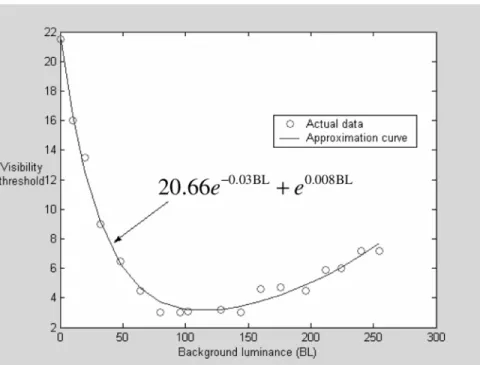
The schematic block diagram of the proposed image reso-lution enhancement system is shown in Fig. 1. The proposed system consists of a fuzzy decision module, an angel evaluation module, an adaptive neural-network interpolation module, and a bilinear interpolation module. The fuzzy decision module des-ignates each sliding block as shown in Fig. 2, which receives for one of a plurality of predefined classifications. Based on this classification, one of the bilinear interpolation and adaptive neural-network interpolation modules is selected for actuation

in generating the supplementary image pixels necessary to sup-port resolution enhancement. When the adaptive neural network interpolation is actuated, the angle evaluation module will com-pute the dominant orientation of the sliding block in the original image as one of the input data of the proposed neural network.

When an original image enters the proposed system, it is first divided into 4 4 sliding windows that are processed pixel by pixel. The original block is shown in Fig. 2(a) as an illustration, where (1,1) is defined as the reference pixel and is the neighborhood of (1,1). According to Fig. 2(b), the three adjacent image pixels relative to reference image pixel (1,1) are needed to be interpolated and positioned at offset coordinate points (1,0), (0, 1), and (1, 1) in a Cartesian coordinate reference system for the two times interpolation. The weighted interpolation is used and can be presented as

(1)

where the weights are derived from a neural network. This neural network is trained according to the edge angle of the reference image pixel to obtain the corresponding weights. In order to achieve optimal edge-directed interpolation, we make use of the properties of the human visual system to be our foun-dation by which we obtain the features of images. We can also determine which region would be worth processing for us in particular by using the properties of HVS, since human eyes are usually more sensitive to this region.

A. Fuzzy Decision

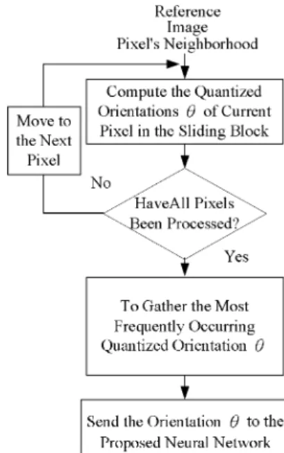
Much research has been done over the years on discovering the characteristics of the HVS. It was found that the perception of HVS is more sensitive to luminance contrast rather than uni-form brightness. The ability of human eyes to tell the magni-tude difference between an object and its background depends on the average value of background luminance. According to Fig. 3, we find that the visibility threshold is lower when the background luminance is within the interval 70 to 150, and the visibility threshold will increase if the background luminance becomes darker or brighter away from this interval. In addition, high visibility threshold will occur when the background lumi-nance is in a very dark region [16].

In addition to the magnitude difference between an object and the background, different structures of images also cause dif-ferent visual perceptions for HVS. Human eyes are more sen-sitive to high-contrast regions such as texture or edge regions than the smooth regions. Since processing speed of interpolation and the resultant quality form a tradeoff, in this paper, a novel fuzzy decision system inspired by HVS is proposed to classify the input image into human perception nonsensitive regions and sensitive regions. For nonsensitive regions, the bilinear interpo-lation is used to reduce the computational cost. For sensitive regions, the proposed adaptive neural network is used to match the characteristics of human visual perception.

In the proposed fuzzy decision system, there are three input variables visibility degree (VD), structural degree (SD), and

Fig. 3. Visibility thresholds corresponding to different background luminance.

complexity degree (CD) and one output variable— (Mo). In order to obtain the input variables corresponding to each sliding block shown in Fig. 2(a), two index parameters called back-ground luminance (BL) [16] and difference (D) are defined and should be calculated first. Parameter BL is the average lumi-nance of the sliding block and can be calculated by

BL (2)

where

(3)

Parameter D is the difference between the maximum pixel value and the minimum pixel value in the sliding block and can be calculated by

D (4)

A nonlinear function V(BL) is also designed to approximate the relation between the visibility threshold and background luminance. It is the approximation of Fig. 3, [16] obtained by

using the nonlinearly recursive approach, and can be repre-sented as

V(BL) (5)

After BL, D, and V(BL) are obtained, we can calculate the input variables (VD, SD, and CD) of the fuzzy decision system. Parameter VD is defined as the difference between D and V(BL) and can be represented as

VD D V(BL) (6)

In (6), “D” value defined in (4) is used to approximate the magnitude difference between the object and its background. Therefore, if VD , it means the magnitude difference between the object and its background exceeds the visibility threshold and the object is sensible. Otherwise, this object is not sensible.

SD and CD are used to indicate whether the pixels in the sliding block perform edge structure. SD shows if the sliding block is a high contrast region and the pixels in the block can be obviously separated into two clusters. It is calculated by (7), as shown at the bottom of the page, where

mean (8)

Fig. 4. An illustration of the relation between SD parameter and the distribution of pixels in a sliding block.

Fig. 5. Portions of (a) the sliding block including texture structure and (b) the sliding block including edge structure.

An illustration of (7) is shown in Fig. 4. According to Fig. 4,

(7) can be expressed as . So the SD has

been normalized to [0, 1] and this rule can also be applied to images with a different intensity range. If SD is small (close to zero) and and are close [see Fig. 4(a)], it means the pixels in the block can be separated into two even clusters. The block may contain edge or texture structure. On the contrary, if SD is a large value [Fig. 4(b)], it means the pixel number of one cluster and that of the other cluster are not even; thus, the block may contain noise or thin line edge

CD

(9)

Fig. 5(a) and (b) shows a texture structure and a delineated edge structure in a sliding block, respectively. In these two plots, pixel numbers of the two clusters are the same. Therefore, the SD values corresponding to these two structures are close. Since the proposed neural network is used to interpolate the sensitive regions such as Fig. 5(b), a CD input variable based on the local gradient process is proposed to tell the delineated edge struc-ture from texstruc-ture strucstruc-ture. It is calculated by (9), where is the binarized version of to eliminate the influence of image intensity. In (9), each pixel in the 4 4 sliding block takes the four-directional local gradient operation, and the CD is the summation of the 16 local gradient values. If the CD is a large value, it means the block may contain texture structure. On the contrary, if the CD is a small value, the block may contain de-lineated edge structure.

The input variable VD has two fuzzy sets N (negative) and P (positive). The input variable SD has three fuzzy sets S (small), M (medium), and B (Big). The input variable CD has three

Fig. 6. Membership functions of fuzzy sets on input variables (a) VD, (b) SD, and (c) CD and (d) output variable Mo.

fuzzy sets S (small), M (medium), and B (Big). The member-ship functions corresponding to the VD, SD, and CD are shown in Fig. 6(a)–(c), respectively. In order to determine the fuzzy membership functions, seven nature images were used to gen-erate the model. The images were separated into smooth, tex-ture, and edge regions by the admission of the majority (seven of ten subjects). Then the ranges of VD, SD, and CD proposed in (6), (7), and (9) corresponding to these regions were evaluated. Finally, the membership functions of VD, SD, and CD could be designed according to the distribution ranges of the parameters in four regions, respectively. The membership functions corre-sponding to Mo are shown in Fig. 6(d). Originally there are 36 fuzzy rules in the proposed fuzzy system (

rules). These fuzzy rules can be combined and reduced in ac-cordance with the following three rules [23].

1) The fuzzy decision rules have exactly the same conse-quence.

2) Some preconditions are common to all the rule nodes in this set.

3) The union of other preconditions of these rules nodes com-poses the whole term set of some input linguistic variables. Therefore, we can combine these 36 fuzzy decision rules into seven rules as follows.

1) If VD is N then Mo is BL. 2) If SD is B then Mo is BL. 3) If CD is B then Mo is BL.

4) If VD is P and SD is S and CD is S then Mo is NN. 5) If VD is P and SD is S and CD is M then Mo is BL. 6) If VD is P and SD is M and CD is S then Mo is NN. 7) If VD is P and SD is M and CD is M then Mo is BL.

The numerical value of Mo after defuzzification by center of area (COA) [23] is compared with a threshold value , where is preferably set as the value five by experiments. The COA strategy generates the center of gravity of the possibility distri-bution for the decision action. In the case of discrete universe, assuming is the number of quantization levels of the output, is the amount of system output at the quantization level , and

represents its membership value in the output fuzzy set, Mo can be calculated by

Fig. 7. Flow diagram of the angle evaluation.

When Mo Th, the adaptive neural-network interpolation module would be chosen; otherwise, the bilinear interpolation module would be used. An example of how to use the proposed fuzzy system for image analysis is presented in Section IV.

B. Angle Evaluation

According to Fig. 1, when Mo , the angle evaluation is performed to determine the dominant orientation of the sliding block. The flow diagram of angle evaluation is shown in Fig. 7. When angle evaluation is operating, the orientation angle of each neighborhood original image pixel is computed. Ac-cording to Fig. 2, when the orientation angle of denoted as is computed, the luminance values of the original pixels nearby are used for the following computations:

(11)

(12) (13)

where and .

The obtained orientation angle of each pixel in the sliding block [as shown in Fig. 2(a)] is quantized into eight quantization

sectors such as degrees, where is

the quantized angle for most pixels oriented in the sliding block and regarded as the dominant orientation of the reference image pixel.

III. NEURAL-NETWORK-BASEDIMAGEINTERPOLATION

A. Conceptions of Neural Network Image Interpolation

In recent years, many edge-directed interpolation algorithms have been proposed to improve the subjectively visual quality

of the resized images [5]–[15]. In this section, the bilinear inter-polation and an artificial neural network are combined to solve these problems.

To use a neural network to solve a problem, two issues should be considered in the first stage: the function of the network and the cost function to minimize (for supervised learning). The function of the proposed neural network is to obtain the weights defined in (1), where represents the quantized dominant orientation of the reference pixel;

therefore, , and represents the

coordinate of the supplementary pixel relative to the reference pixel. Therefore, assuming two-time enlarging is performed, , according to Fig. 2(b). Thus, the proposed neural network is used to obtain 24 (8 3) sets of weighting matrices through training. Each weighting matrix can be represented as

(14)

In order to use supervised learning algorithms to train the proposed neural network, we have to obtain the desired input– output patterns such that the differences of network outputs and the corresponding desired outputs can be used to define the cost function as the goal to minimize. In this section, several high-resolution images are used as training patterns. Assuming a high-resolution image is denoted as and it is downsampled by two to get a new image denoted as , where

and . Therefore, can be regarded as

the input image for interpolation and is the desired output for the two-time enlarging process. Since the nonorientated re-gions are interpolated by the bilinear method in our system, only sensitive and orientated regions of with dominant orien-tation are used for training. According to Fig. 2(b), let be the reference pixel, where , and it is clas-sified as an edge pixel with dominant orientation after angle evaluation. The supplementary pixels that need to be

interpo-lated are , where .

The input vector of the neural network can be defined as and the network output is the pixel value of . Then the desired output can be the pixel value of obtained from the original high-resolution image.

B. Architecture of the Neural Network for Image Interpolation

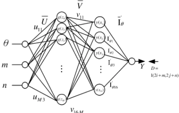
Since the input–output patterns are given, the following task is designing a neural network to match the input–output rela-tions. A new neural network as shown in Fig. 8 is proposed for image interpolation. It is a four-layer network with two hidden layers. The input layer consists of three nodes corresponding to , and , respectively. The second layer (first hidden layer) consists of M nodes denoted as , and the bipolar sigmoid function is used as the activation function. The weighting vector between the first and the second layer is denoted as . The third layer (second hidden layer) includes 16 nodes and the bipolar sigmoid function also performs as the activation function. The

Fig. 8. The proposed feedforward neural network for image interpolation.

weighting vector between the second and the third layers is de-noted as . The output value of each node in the third layer is de-noted as and represents an element of the weighting matrix given in (14), where

, and . The fourth layer is the output layer with one output node, and its output value represents the interpolated pixel value of the supplementary pixel . The weighting vector between the third and the fourth layers is denoted as . It represents the neighborhood of the reference pixel with dominant orientation as follows:

..

. ...

(15)

The system output can be calculated by

(16)

and the corresponding desired output can be obtained by (17) It should be noted that the weighting vectors need to be updated in the training stage are only and . If a reference pixel is given, the weighting vector is also determined. Therefore, it can be regarded as an extra input vector. This unique operating rule is the major difference between the proposed network and the common feedforward networks and is specially designed for the image-interpolation application.

In the training stage, the updating rules of weights can be derived by the backpropagation method as

(18)

TABLE I

THEEIGHTWEIGHTINGMATRICESOBTAINEDFROM THETRAINED

NEURALNETWORK

(19)

When the training process is finished, the weighting vectors ( and ) of the neural network are obtained and fixed. Then 24 different input patterns can be inputted to the trained network, and the output value of each node in the third layer corresponding to each input pattern represents an ele-ment of the weighting matrix . We can collect the ob-tained 24 weighting matrices to build a lookup table combined with (1) for image interpolation to reduce the com-putational cost.

Fig. 9. Portions of original image (a) Lena, (b) Home, (c) Lighthouse, and (d) Goldhill.

IV. EXPERIMENTALRESULTS ANDDISCUSSIONS

In our experiments, 30 high-resolution natural images are used to train the proposed neural network. These images are color images in the 24-bit RGB format. The goal of training stage is to reduce the cost function [mean squared error (MSE)] to 1% of the intensity range, i.e., . In our ex-periments, 200 nodes in the first hidden layer were required to achieve this goal due to the variations of the training im-ages and the selected training portions, and the learning rate was 0.2. The edge regions in these training images are sepa-rated into eight different quantized angles. The variations may be caused by the quantization error (11.25 ) and the character-istics of different images and regions. In addition, the vector between the third and the fourth layers of the neural network for image quality enhancement represents the 16 neighborhood pixels of the reference pixel. If we release the goal (MSE) to achieve from 2.5 to 5, the hidden nodes in the first hidden layer can be reduced to 80 without affecting the visual quality heavily. After training, weighting matrices are obtained for testing. The weighting matrices correspond to eight different edge ori-entations for the three supplementary pixels in Fig. 2(b) are pre-sented in the Table I. We analyze the weighting matrices corre-sponding to in Fig. 2(b) as an example. In Table I(a), W1 and W3 look like the rotated versions of W5 and W7, re-spectively. The rest of the weighting matrices W2, W4, W6, and W8 look like the rotated versions of each other. The similar phe-nomenon can also be observed in Table I(b) and (c). It means the proposed neural network can catch the directional characteris-tics of edges through automatic training.

1_{Signal Analysis and Machine Perception Laboratory, Ohio State University,}

http://sampl.eng.ohio-state.edu/sampl/.

Fig. 10. Portions of resolution enhanced Lena image by (a) bilinear interpo-lation, (b) bicubic interpointerpo-lation, (c) linear associative memories (LAM) inter-polation [15], (d) edge-directed interinter-polation [14], (e) AQua interinter-polation [12], and (f) the proposed HVS-directed NN-based interpolation.

Six natural photographic images1_{are used as our benchmark} images for testing and are not included in the training data to demonstrate the generalization ability: Lena, Home, Goldhill,

Lighthouse, Barbara, and Peppers. In our experiments, the

pro-posed HVS-directed image interpolation is compared with two conventional interpolation methods, the bilinear and the bicubic, and three modern interpolation methods, the neural-network-based interpolation method [15], the edge-directed interpola-tion [12], and adaptively quadratic (AQua) interpolainterpola-tion [14].2 Fig. 9(a)–(d) shows the portions of original images Lena, Home,

Lighthouse, and Goldhill for testing in our experiments. Their

two-time enlargement images by using different interpolation methods are shown in Figs. 10–13, according to which it can be found that the bilinear interpolation made some jaggedness along the edges and blurred the image. The images interpolated by the bicubic method were less blurring than the result of the bilinear method, but the bicubic method made more observable

Fig. 11. Portions of resolution enhanced Home image by (a) bilinear interpo-lation, (b) bicubic interpointerpo-lation, (c) LAM interpolation [15], (d) edge-directed interpolation [14], (e) AQua interpolation [12], and (f) the proposed HVS-di-rected NN-based interpolation.

jagged edges. The results of the neural-network-based interpo-lation method [15] were less blurring than the result of bilinear method, and this neural-network-based method made less vis-ible jaggedness than the bicubic method. The edge-directed in-terpolation [12] produced some serious distortion to destroy the visual perception, while the AQua interpolation [14] made less distortion but the results were still more blurring than those of the proposed method. Table II shows the quantitative com-parisons of different interpolation technologies. According to the experimental results, the proposed HVS-directed neural-net-work-based interpolation is superior to the other interpolation methods both in the quantitative performance [such as MSE and peak signal-to-noise ratio (PSNR)] and visual qualitative performance (such as the clarity and the smoothness in edge regions). We have also examined the experimental results on many display devices such as cathode-ray tube monitors, liquid crystal display, projectors, and printers. The consistent quality improvement of visual perception can be obviously observed on these different devices.

In the case of four-time enlargement, the resolution enhanced image can be obtained by operating the two-times enlargement scheme two times. In the case of three-times enlargement, the coordinate positions of eight pixels denoted as (2/3,0), (4/3,0), (0, 2/3), (2/3, 2/3), (4/3, 2/3), (0, 4/3), (2/3, 4/3), (4/3, 4/3) can be fed into the trained neural network to get the

Fig. 12. Portions of resolution enhanced Lighthouse image by (a) bilinear inter-polation, (b) bicubic interinter-polation, (c) LAM interpolation [15], (d) edge-directed interpolation [14], (e) AQua interpolation [12], and (f) the proposed HVS-di-rected NN-based interpolation.

corresponding weighting matrices of each supplementary pixel needed to be interpolated for image resizing.

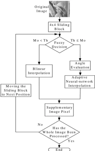
Fig. 14 shows four different image structures extracted from

Home to illustrate the operations of the proposed fuzzy decision

system. Fig. 14(a)–(d), represents smooth, texture, edge, and noise regions, respectively. The VD, SD, and CD values of these regions calculated by (6)–(9) are shown in Table III.

According to the VD values in Table III, only Fig. 14(a) (smooth region) is negative, which activates fuzzy rule 1 and follows the assumption that “if VD , it contains visible objects.” The SD value of Fig. 14(d) (noise) is large (B), which activates fuzzy rule 2 and follows the assumption that “If SD is a large value, the block may contain noise.” The SD values of Fig. 14(b) (texture region) and Fig. 14(c) (edge region) are small (S), which follows our assumption that “if SD is small, the block may contain edge or texture structure. The CD value of Fig. 14(b) is medium (M), which activates fuzzy rules 5 and it follows the assumption that “If CD is a large value, the block may contain texture structure.” The CD value of Fig. 14(c) is small (S), which activates fuzzy rule 4 and follows the assump-tion that “If CD is a small value, the block may contain edge structure.”

After defuzzification, their Mo values are 2.2, 3.4, 7.3, and 2.2, respectively. Since the threshold value is five, only the edge

TABLE II

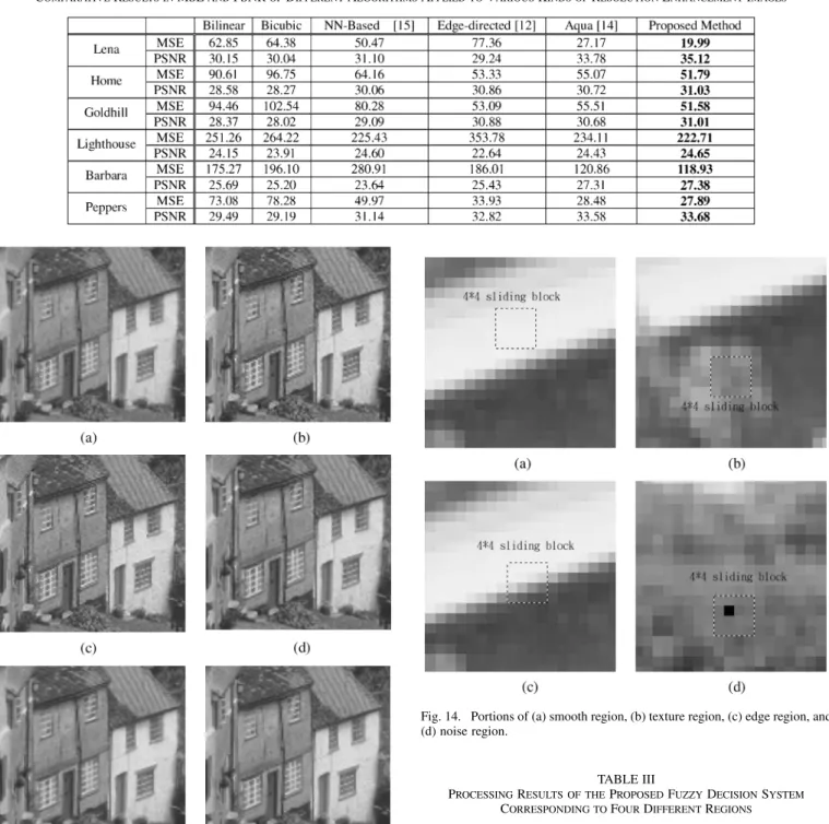
COMPARATIVERESULTS INMSEANDPSNROFDIFFERENTALGORITHMSAPPLIED TOVARIOUSKINDS OFRESOLUTIONENHANCEMENTIMAGES

Fig. 13. Portions of resolution enhanced Goldhill image by (a) bilinear interpo-lation, (b) bicubic interpointerpo-lation, (c) LAM interpolation [15], (d) edge-directed interpolation [14], (e) AQua interpolation [12], and (f) the proposed HVS-di-rected NN-based interpolation.

region shown in Fig. 14(c) is interpolated by the proposed neural network. The threshold value can be adjusted to meet the speed and quality requirements of different applications.

V. CONCLUSION

In this paper, a novel HVS-directed interpolation algorithm based on the artificial neural network was proposed. The fuzzy

Fig. 14. Portions of (a) smooth region, (b) texture region, (c) edge region, and (d) noise region.

TABLE III

PROCESSINGRESULTS OF THEPROPOSEDFUZZYDECISIONSYSTEM

CORRESPONDING TOFOURDIFFERENTREGIONS

decision rules inspired by human visual system were proposed to analyze the sensitivity of human eyes to the image for interpolation. A new neural network was proposed for image interpolation and high-resolution nature images combined with backpropagation training methods to train the proposed neural network. According to the experiment results, the proposed HVS-directed NN-based interpolation is superior to conven-tional methods and three modern interpolation methods in some

aspects of visual quality, such as the clarity and the smoothness in edge regions as well as the visual quality of the interpolated images. In addition, the proposed fuzzy decision rules com-bined with the neural network can balance the tradeoff between speed and quality for different applications by just adjusting a threshold parameter.

REFERENCES

[1] K. Xue, A. Winans, and E. Walowit, “An edge-restricted spatial inter-polation algorithm,” J. Electron. Imag., pp. 152–161, 1992.

[2] M. Unser, A. Aldroubi, and M. Eden, “Enlargement or reduction of digital images with minimum loss of information,” IEEE Trans. Image

Process., vol. 4, pp. 247–258, 1995.

[3] K. Jensen and D. Anastassiou, “Subpixel edge localization and the in-terpolation of still image,” IEEE Trans. Image Process., vol. 4, pp. 285–295, 1995.

[4] H. C. Ting and H. M. Hang, “Spatially adaptive interpolation of digital images using fuzzy inference,” in Proc. SPIE Visual Commun. Image

Process., 1996, pp. 1206–1217.

[5] J. E. Adams, “Interactions between color plane interpolation and other image processing functions in electronic photography,” in Proc. SPIE, 1995, vol. 2416, pp. 144–151.

[6] S. W. Lee and J. K. Paik, “Image interpolation using adaptive fast b-spline filtering,” in Proc. IEEE Int. Conf. Acoust., Speech, Signal

Process., 1993, vol. 5, pp. 177–180.

[7] B. S. Morse and D. Schwartzwald, “Isophote-based interpolation,” in

Proc. IEEE Int. Conf. Image Process., 1998, vol. 3, pp. 227–231.

[8] K. Ratakonda and N. Ahuja, “POCS based adaptive image magnifi-cation,” in Proc. IEEE Int. Conf. Image Process., 1998, vol. 3, pp. 203–207.

[9] D. Call and A. Montantanvert, “Superresolution inducing of an image,” in Proc. IEEE Int. Conf. Image Process., 1998, vol. 3, pp. 232–235. [10] J. Allebach and P. W. Wong, “Edge-directed interpolation,” in Proc.

IEEE Int. Conf. Image Process., 1996, vol. 3, pp. 707–710.

[11] S. Carrato, G. Ramponi, and S. Marsi, “A simple edge-sensitive image interpolation filter,” in Proc. IEEE Int. Conf. Image Process., 1996, vol. 3, pp. 711–714.

[12] X. Li and M. T. Orchard, “New edge-directed interpolation,” IEEE

Trans. Image Process., vol. 10, pp. 1521–1527, 2001.

[13] D. D. Muresan and T. W. Parks, “Adaptive, optimal-recovery image in-terpolation,” in 2001 IEEE Int. Conf. Acoust., Speech, Signal Process., 2001, vol. 3, pp. 1949–1952.

[14] ——, “Adaptively quadratic (AQua) image interpolation,” IEEE Trans.

Image Process., vol. 13, no. 5, pp. 690–698, 2004.

[15] F. M. Candocia and J. C. Principe, “Super-resolution of images based on local correlations,” IEEE Trans. Neural Netw., vol. 10, no. 2, pp. 372–380, 1999.

[16] C. H. Chou and Y. C. Li, “A perceptually tuned subband image coder based on the measure of just-noticeable-distortion profile,” IEEE Trans.

Fuzzy Syst., vol. 3, no. 3, 1995.

[17] C. I. Podilchuk and W. Zeng, “Image-adaptive watermarking using vi-sual models,” IEEE J. Sel. Areas Commun., vol. 16, no. 4, pp. 525–539, May 1998.

[18] C. S. Lu, S. K. Huang, C. J. Sze, and H. Y. M. Liao, “Cocktail water-marking for digital image protection,” IEEE Trans. Multimedia, vol. 2, no. 4, pp. 209–224, Dec. 2000.

[19] H. Lin and A. N. Venetsanapoulos, “Incorporating human visual system (HVS) models into the fractal image compression,” in Proc.

1996 IEEE Int. Conf. Acoust., Speech, Signal Process., 1996, vol. 4,

pp. 1950–1953.

[20] Y. Chee and K. Park, “Medical image compression using the charac-teristics of human visual system,” in Proc. IEEE 16th Annu. Int. Conf., 1994, vol. 1, pp. 618–619.

[21] M. Bertran, J. F. Delaigle, and B. Macq, “Some improvements to HVS models for fingerprinting in perceptual decompressors,” in 2001 Int.

Conf. Image Process., 2001, vol. 2, pp. 1039–1042.

[22] J. F. C. Wanderley and M. H. Fisher, “Color texture invariants for natural image recognition based on human visual system,” in

Proc. 7th IEEE Int. Conf. Electron., Circuits Syst., 2000, vol. 1, pp.

295–298.

[23] C. T. Lin and C. S. G. Lee, Neural Fuzzy Systems: A Neuro-Fuzzy

Syn-ergism to Intelligent Systems. Englewood Cliffs, NJ: Prentice-Hall, 1996.

[24] C. T. Lin, Y. C. Lee, and H. C. Pu, “Satellite sensor image classifica-tion using cascaded architecture of neural fuzzy network,” IEEE Trans.

Geosci. Remote Sens., vol. 38, no. 2, pp. 1–11, Mar. 2000.

[25] C. T. Lin, I. F. Chung, and L. K. Sheu, “A neural fuzzy system for image motion estimation,” Fuzzy Sets Syst., vol. 114, no. 2, pp. 281–304, Sept. 2000.

[26] C. T. Lin, Neural Fuzzy Control Systems With Structure and Parameter

Learning. Singapore: World Scientific, 1994.

[27] M. S. Longuet-Higgins, “Statistical properties of an isotropic random surface,” Phil. Trans. Roy. Soc. A, pp. 151–171, 1957.

[28] N. Memon and X. Wu, “Recent developments in context-based predic-tive techniques for lossless image compression,” Comput. J., vol. 40, no. 2/3, pp. 127–136, 1997.

[29] H. Derin and H. Elliot, “Modeling and segmentation of noisy and tex-tured images using Gibbs random field,” IEEE Trans. Pattern Anal.

Machine Intell., vol. 9, pp. 39–55, 1987.

[30] Y. H. Lee and S. Tantaratana, “Decision-based order statistics filters,”

IEEE Trans. Acoust., Speech, Signal Process., vol. 38, pp. 406–420,

Mar. 1990.

[31] J. W. Woods, “Two-dimensional discrete markovian fields,” IEEE

Trans. Inf. Theory, vol. IT-18, pp. 232–240, 1972.

[32] A. Said and W. A. Pealrman, “A new, fast and efficient image codec based on set partitioning of hierarchical trees,” IEEE Trans. Circuits

Syst. Video Technol., vol. 6, pp. 243–250, 1996.

Chin-Teng Lin (F’05) received the B.S. degree from National Chiao-Tung University (NCTU), Taiwan, R.O.C., in 1986 and the Ph.D. degree in electrical engineering from Purdue University, West Lafayette, IN, in 1992.

He is currently the Chair Professor of Electrical and Computer Engineering, Dean of the Computer Science College, and Director of the Brain Research Center, NCTU. He was Director of the Research and Development Office, NCTU, from 1998 to 2000, Chairman of the Electrical and Control Engineering Department, NCTU, from 2000 to 2003, and Associate Dean of the College of Electrical Engineering and Computer Science from 2003 to 2005. His current research interests are fuzzy neural networks, neural networks, fuzzy systems, cellular neural networks, neural engineering, algorithms and VLSI design for pattern recognition, intelligent control, and multimedia (including image/video and speech/audio) signal processing, and intelligent transportation systems. He is coauthor of Neural Fuzzy Systems—A Neuro-Fuzzy Synergism to Intelligent

Systems (Englewood Cliffs, NJ: Prentice-Hall, 1996) and the author of Neural Fuzzy Control Systems with Structure and Parameter Learning (Singapore:

World Scientific, 1994). He has published more than 90 journal papers in the areas of neural networks, fuzzy systems, multimedia hardware/software, and soft computing, including about 60 IEEE journal papers. He is an Associate Editor of the International Journal of Speech Technology.

Dr. Lin is a member of Tau Beta Pi, Eta Kappa Nu, and Phi Kappa Phi. He was a member of the Board of Governors, IEEE Circuits and Systems (CAS) Society, in 2005 and the IEEE Systems, Man, Cybernetics (SMC) Society in 2003-2005. He was a Distinguished Lecturer of the IEEE CAS Society from 2003 to 2005. He is the International Liaison of the International Symposium of Circuits and Systems (ISCAS) 2005 in Japan, Special Session Cochair of ISCAS 2006 in Greece, and Program Cochair of the IEEE International Con-ference on SMC 2006 in Taiwan. He has been President of the Asia Pacific Neural Network Assembly since 2004. He received the Outstanding Research Award from the National Science Council, Taiwan, in 1997, the Outstanding Electrical Engineering Professor Award from the Chinese Institute of Electrical Engineering in 1997, the Outstanding Engineering Professor Award from the Chinese Institute of Engineering in 2000, and the 2002 Taiwan Outstanding In-formation-Technology Expert Award. He was elected one of the 38th Ten Out-standing Rising Stars in Taiwan (2000). He currently is an Associate Editor of IEEE TRANSACTIONS ONCIRCUITS ANDSYSTEMS—PARTI: REGULAR PA-PERS ANDPARTII: EXPRESSBRIEFS, IEEE TRANSACTIONS ONSYSTEMS, MAN, CYBERNETICS, IEEE TRANSACTIONS ONFUZZYSYSTEMS.

Kang-Wei Fan was born in Hsinchu County, Taiwan, R.O.C., on June 1, 1976. He received the M.S degree in computer science and information engineering from Chung Hua University, Hsinchu, Taiwan, in 2002. He is currently pursuing the Ph.D. degree in electrical and control engineering from National Chiao Tung University, Hsinchu.

His research interests are in the areas of digital image, video processing, and color science.

Her-Chang Pu was born in Taipei, Taiwan, R.O.C., in 1972. He received the B.S. and M.S. degrees in au-tomatic control engineering from Feng-Chia Univer-sity, Taichung, Taiwan, in 1998 and the Ph.D. degree in electrical and control engineering from National Chiao-Tung University (NCTU), Hsinchu, Taiwan, in 2003.

Currently, he is a Research Assistant Professor in electrical and control engineering, NCTU. His current research interests are in the areas of artificial neural networks, fuzzy systems, pattern recognition, machine vision, and intelligent transportation systems.

Shih-Mao Lu received the B.E. degree in power mechanical engineering from Tsing Hua University, Taiwan, R.O.C., in 1998 and the M.E. degree in electrical control engineering from Chiao Tung University, Hsinchu, Taiwan, in 2000, where he is currently pursuing the Ph.D. degree in electrical control engineering.

His research interests include image processing, noise and compression coding artifacts suppression, visual quality assessment, human vision system, and applications of neural networks and fuzzy theory.

Sheng-Fu Liang was born in Tainan, Taiwan, R.O.C., in 1971. He received the B.S. and M.S. degrees in control engineering and the Ph.D. degree in electrical and control engineering from National Chiao-Tung University (NCTU), Taiwan, in 1994, 1996, and 2000, respectively.

From 2001 to 2005, he was a Research Assistant Professor in the Electrical and Control Engineering Department, NCTU. In 2005, he joined the Depart-ment of Biological Science and Technology, NCTU, where he is an Assistant Professor. He has been Chief Executive of the Brain Research Center, NCTU Branch, University System of Taiwan since September 2003. His current research interests are biomedical en-gineering, biomedical signal/image processing, machine learning, fuzzy neural networks, the development of brain–computer interface, and multimedia signal processing.