An efficient method for creating benchmark classifications for automatic workpiece classification systems

(1)

An

M od

for Creating nchmark

Class ns

for

Automatic Workplece Clasaifica n

Systems

S. H. Hsu, T. C. Hsia and M. C. Wu

Department of Industrial Engineering and Management, National Chiao Tung University, Hsinchu, Taiwan

The usefulness of an automatic workpiece classification system depends primarily on the extent to which its classification results are consistent with users' judgements. Thus, to evaluate the effectiveness o f an automatic classification system it is necessary to establish classification benchmarks based on users' judgements. Such benchmarks are typically established by having subjects perform pair comparisons o f all workpieces in a set of sample workpieces. The result of such comparisons is called a full-data classification. However, when the number of sample workpieces is very large, such exhaustive compari- sons become impractical. This paper proposes a more efficient method, called lean classification, in which data on compari- sons between the samples and a small number of typical workpieces are used to infer the complete classification results. The proposed method has been verified by using a small set of 36 sample workpieces and by computer simulation with medium to large sets of 100 to 800 sample workpieces. The results reveal that the method could produce a classification that was 71% consistent with the full-data classification while using only 10% of the total data.

Keywords: Automatic workpiece classification system; Classi-

fication benchmarks; Full-data classification; Lean classification

1. Introduction

Group technology (GT) refers to techniques by which workpieces with similar shape, size, or manufacturing requirements are grouped into families in order to enhance design and manufacturing productivity. Early GT methods, which were based primarily upon manual classification of the similarity of workpiece attributes, were complicated, time-consuming, and error-prone. Since then considerable research has been carried out on automatic classification of workpieces [1-4]. However, the methods thus developed still employ only the local shapes

Correspondence and offprint requests to: Dr Shang H. Hsu, Depart- ment of Industrial Engineering and Management, 1001 Ta-Hsueh Road, Hsinchu, Taiwan, E-maih shhsu@cc.nctu.edu.tw.

of workpieces as classification criteria and have two major shortcomings:

1. Similarity in local geometric features does not necessarily entail similarity in global shape.

2. Methods based on local shape are less applicable during the design phase, because a designer's conceptual model tends to develop from an overall picture to local details. Thus, methods that use local shape attributes as workpiece classification criteria are generally limited in global shape retrieval applications.

More recent GT work has begun to characterise workpieces on the basis of global shape and to apply automatic classification systems [5-7]. This approach does not focus on local attributes but on the overall contour of workpieces. Focusing on the overall contour enhances the usefulness of workpiece classification for conceptual design work and can help to improve efficiency in manufacturing and assembly. A key concept in choosing an effective automatic workpiece classification system for design, manufacturing, and assembly applications is the degree of consistency between the classification results and users' judgements. To help ensure a high level of consistency, benchmarks based on user classification must be established with which to measure the performance of automatic workpiece classification systems.

To establish such classification benchmarks, Hsu et al. [8] presented a full-data classification technique, in which a set of sample workpieces are selected from the general population of workpieces, and subjects make pair comparisons of each pair of sample workpieces on the basis of the similarity of the global shape of the workpieces. The degree of similarity between each pair of sample workpieces is obtained from the overall results of the user comparisons, and these data are used to classify the samples. The classification results can be regarded as a benchmark for classifications of the sample workpieces. By comparing these classification results with those of various automatic classification systems for the same set of samples, one can identify an automatic classification system that pro- duces results most consistent with users' judgements. Yet full-data classification is also problematic, because it requires exhaustive pair comparisons of all of the sample workpieces. If the number of workpieces is n, and the number of compari-

(2)

482 S. H. Hsu et al.

sons that must be made is at least n ( n - 1)/2. That is, the testing needed to classify a large set of sample workpieces will be extremely time-consuming. Moreover, when experimental subjects are required to make a very large number of pair comparisons, they are likely to become fatigued and to produce biased or inconsistent judgements.

The aim of the research reported here was to develop a "lean classification" method that reduces shortcomings of full- data classification by maintaining classification accuracy while reducing the number of comparisons needed to produce a classification of the sample workpieces. In this method, partial experimental data obtained from pair comparisons of each sample workpiece with a small number of typical workpieces are used instead of exhaustive data obtained by comparing every pair of sample workpieces. If it performs as intended, this method will yield a classification that was 71% consistent with the full-data classification while using only 10% of the total data.

2. Experiments to Collect Lean

Classification and Full-Data Classification

Data

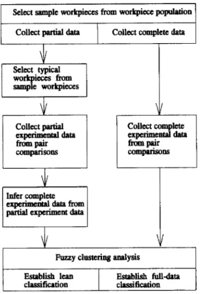
An experimental study was carried out to collect pair similarity comparison data for a set of 36 sample workpieces. These data were then used to establish a lean classification and a full- data classification. The procedure followed is outlined in Fig. 1.

2.1 Selecting Sample Workpleces from the

Workplace Population

In an automatic workpiece classification system, if a large number of workpieces must be classified, there are likely to be a large number of workpiece categories. In this research, a comparatively small number of workpieces were chosen from the general workpiece population and the similarity of these sample workpieces was compared manually to establish a classification benchmark. Sample workpieces were selected according to a stratified sampling method [9]. A broad estimate was made of the number of workpiece categories likely to be appropriate in the practical environment in which an automatic classification system is used, the number of workpieces in each category was estimated, and then sample workpieces were selected from the general population according to the proportion of the number of workpieces in each category. For instance, suppose there are nine categories of workpieces in a certain design and manufacturing environment and there are approxi- mately the same number of workpieces in each of these nine categories. Then if we randomly select four workpieces from each category, the total number of sample workpieces will be 36 (see Fig. 2). (For convenience, this set of 36 sample workpieces will be used as an example for the remainder of the paper.)

2.2 Selecting Typical Workpleces from Sample

Workpieces

Select sample workpieces from workpiece population Collect partial Select typical workpieces from sample workpieces Collect partial expetimeml aata from pair comparisons

Collect complete data

Collect complete

Infer complete I

experimemJ a m from I partial experiment data

Fuzzy clustering analysis

Establish lean Establish full-data classificadon classification

Fig. 1. Procedure for establishing lean classification and full-data classification.

In a practical environment, if there are an excessive number of sample workpieces, then it will be time-consuming and costly to carry out complete experimental comparisons of the workpieces. Consider a set of 1000 sample workpieces; complete experimental testing would involve about 0.5 million pair comparisons (i.e. C~°°°). If each of these comparisons took 10 seconds and the subjects worked 8 hours a day, it would take 173 working days to complete the comparison. Even a set of 36 sample workpieces would involve 630 individual comparisons. In place of this exhaustive testing, the proposed method is to select a small number of typical workpieces with different shapes from among the sample workpieces, and then to compare each of these typical workpieces with each of the sample workpieces to obtain partial comparison data. Then these partial data are extrapolated to estimate the results of the complete experimental data for all of the samples. The classification results obtained by using the estimated data are called the lean classification. The degree of consistency between the lean classification and the full-data classification will indicate the effectiveness of the method used to produce the lean classification.

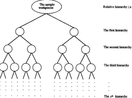
Typical workpieces are selected from among the sample workpieces by using a binary clustering method. First, the sample workpieces are classified by selecting a user at random and having the user hierarchically divide the workpieces into subgroups on the basis of the similarity of their global shape (see Fig. 3). Secondly, groups in the hierarchy are selected at random according to the number of typical workpieces needed: when a lean classification is to be established, the exact number

(3)

Efficient Benchmark Classifications 483 , i | ? / 3

~!i'.

[ ! ! ~ i ~ ~ I 11 ; i

6 i 2

W O d ~ m

Wo~p~

17 2~

~5

. , o

Fig. 2. The 36 sample workpieces used in this research.

The ftrst hierarchy

The second hierarchy

The third hierarchy

. . . o • . , . . . .

. . . The x* hierarchy

Fig. 3. Selecting typical workpieces from sample workpieces by binary clustering. Relative hierarchy (h)

of groups sampled from the relative hierarchy (h) will depend on the number of typical workpieces (m) required. The relation between m and h can be expressed by 2 h- ~ < m <- 2 h. Then one workpiece is chosen at random from each selected group, and the resulting workpieces are used as the typical workpieces. For example, if a lean classification is to be established on the basis of six typical workpieces, then the typical workpieces should be randomly selected from any six of the eight groups in the third level of the hierarchy (see Fig. 3). Selecting typical workpieces from different groups in this way helps to ensure that there are significant differences between the typical workpieces.

2.3 Pair Similarity Comparison between Typical

and Sample Workpisces

For the proposed classification method to be effective, it must be based on accurate data concerning users' judgements of the relative similarity of the typical and sample workpieces. For this reason, a number of subjects were randomly selected from among employees in various departments of a factory using an automatic workpiece classification system. Each subject was asked to compare each typical workpiece with each sample workpiece on the basis of the similarity of their global shape. A classification based on human judgement is likely to lack

(4)

484 S. 1t. Hsu et aL

clear-cut boundaries between categories [10], Therefore, when each pair of workpieces was presented for comparison, subjects were asked to use fuzzy linguistic terms in comparing the degree of similarity between the workpieces. Each linguistic term can be regarded as a fuzzy number, so the comparison data from each subject can be aggregated through operations with fuzzy number arithmetic. After defuzzification of these aggregated fuzzy numbers, a crisp value can be obtained to represent the degree of similarity between any two tested workpieces. The procedure for comparing the similarity of the workpieces involves the following issues:

1. The manner in which the workpieces are displayed. 2. The definition of the linguistic terms of comparison. 3. The aggregation of the comparison results from each subject. 4. The determination of crisp values from the aggregated com-

parison data.

Each of these issues is discussed below.

2.3.1 Display of the Workpieces

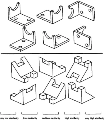
To provide global information concerning the shape of each workpiece and to prevent incorrect judgements in the pair comparisons, each workpiece was displayed by using six isometric views: front, back, top, bottom, left, and right sides (see Fig. 4).

2.3.2 Definition of Terms of Comparison

Subjects provided comparison data by selecting linguistic terms to describe the degree of similarity between each pair of workpieces. The linguistic terms, based on Chen and Hwang's

I ~ 1 I I I t I ... J I ,,1

v~.¢ low similarity low aimikmty rea~ittra similarity kish ~ailnfity vca'y tfilgh Jimik~fity

Fig. 4. Workpieces represented in six isometric views for comparison.

suggestions [11], are treated as five fuzzy numbers: very low similarity, low similarity, medium similarity, high similarity, and very high similarity.

2.3.3 Aggregation of Subjects' Comparison Results

The linguistic terms chosen by the subjects after comparison of each pair of workpieces were aggregated by using the following formula [12]:

where (~

®

represents addition of fuzzy numbers represents multiplication of fuzzy numbers represents the membership function of the linguistic term chosen by the kth subject comparing the similarity of the ith and the jth workpieces, k = 1 . . . w, w = number of subjects

represents the membership function after aggregation of w subjects' comparisons of the ith and jth workpieces

2.3.4 Determining Crisp Values from Aggregated Data

The value of the membership function obtained by aggregating the data for all subjects' comparisons of a pair of workpieces is still a fuzzy number, and it is difficult to perform numerical operations with fuzzy numbers. Hence, for convenience in handling the aggregated comparison data, these values can be transformed into crisp numbers through a defuzzification process. In this research, the aggregated fuzzy numbers were defuzzified by applying the centre of gravity method as follows [13]:

Xc(,)=Ii xlx'-(x)dx

'1 (2)

j ~x)dx

0

where S~ represents a fuzzy number

x represents any element of the fuzzy number in the interval [0, 1 ]

IxXx) represents the membership function of x in the fuzzy set

Xa(~) represents the crisp value of

2.4 Using Partisi Experimental Data to Infer

Complete Experimental Data

This section describes a method for using partial experimental data to infer complete experimental data. The aim is to use the known data obtained from pair comparisons between each typical workpiece and all of the sample workpieces to infer unknown data concerning the degree of similarity between all of the non-typical workpieces. The combination of the known and inferred data will then be equivalent to using complete experimental data.

(5)

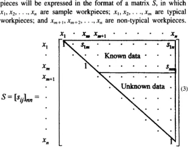
Efficient Benchmark Classifications 485 For convenience, the levels of similarity between all work-

pieces will be expressed in the format of a matrix S, in which x~, x2 . . . x, are sample workpieces; x~, x2 . . . Xm are typical workpieces; and x,~+ i, x,,+2 . . . x , are non-typical workpieces.

S = [sol,," = X I x ~ Xm+l X n x I x . , x=+ l x . - - , ,,,, , , , • ~ - K n o w n d a t a - - •

1 ]~ .

. . . .

s.

(3)

In equation (3), an element s~ of matrix S represents the degree of similarity between x~ and xj. Because s~i =~)~ and s. = l, the matrix is symmetric. Therefore, only the upper part of the data need be considered. In so, if i = l, 2 . . . m and j = i + 1 . . . n, then the elements in the trapezoid part are known data and the elements in the remaining triangular part are unknown data. The structure of the inference is discussed below and then this structure is used to determine the unknown data with the max-min method.

2.4.1 Inference Structure

The basic method used in this research is to infer unknown data about similarity levels between non-typical workpieces by using the degree of similarity between two workpieces and a third workpiece to infer the degree of similarity between the two workpieces. As shown in Fig. 5(a), according to known data, the degree of similarity between a typical workpiece xk and a non-typical workpiece xp is spk and that between xk and another non-typical workpiece Xq is Skq. The inference method proposed here allows us to estimate Spq, the degree of similarity between x , and Xq. This degree of similarity will be denoted by Spq~k), which means that the degree of similarity between xp and Xq will be derived from the typical workpiece xk.

Because there are m typical workpieces, each unknown S~,q can be inferred from m typical workpieces; that is, Spq~k), k = 1, 2 . . . m. To use the existing data to infer the degree

(a)

_(b)

l l q

Spq(k) = Spk (') S kq $pq = A G G Spq(k )

k = l

Fig. 5. s ~ is inferred from m similarity levels between xp and xq.

of similarity between xp and Xq, mathematical methods must be used to aggregate these m data, as shown in Fig. 5(b). Accordingly, the above-mentioned inference process can be described as follows: where m Spq = A G G Spk Q) Skq k = l m = A G G Spq(k ) (4) k - I ® A G G S p k Skq Spq~k~ Spq

represents the inference method represents the method of aggregation

represents the degree of similarity between xp and xk

represents the degree of similarity between xk and xq

represents the degree of similarity between Xp and Xq, which is inferred from k typical work- pieces

represents the degree of similarity between two non-typical workpieces xp and Xq, which is inferred from m typical workpieces. 2,4,2 Using the Max-Min Method to Infer Unknown Data

Fuzzy set theory is used to infer the unknown data. First, the global shape attributes of each typical workpiece are used as a template. The global shape similarity between any two non- typical workpieces and this template can be regarded as a fuzzy relation between these non-typical workpieces and the template, with a value of [0, t]. Secondly, the degree of similarity between the two non-typical workpieces can be inferred by performing max-min composition of the fuzzy relation between the two non-typical workpieces and all typical workpieces. Finally, this method can then be used to infer the degree of similarity between all non-typical workpieces.

The max-min composition of two fuzzy relations is defined as follows [14].

Definition 1: Suppose ~ is a fuzzy relation on the Cartesian product X X Y and ,~ is a fuzzy relation on Y × Z. Then the max-rain composition of/~ and S, denoted b y / ~ o 5, is a fuzzy relation on X x Z and the membership functions

IXaoS-(X,Z) = max rain [ ~ ( x , y ) , Izs.(y,z)]

y e Y

( V x e X, z E Z)

The above definition can be used to infer unknown data on degrees of similarity between non-typical workpieces. We can let K - - {x~,x2 . . . x,.} be a referential set of typical work- pieces and P = Q = {x,,+~, xm+2 . . . x,,} be a referential set o f non-typical workpieces. Suppose SeK = [s~]~ . . . . )m is a fuzzy relation on P x K in which p = m + 1 . . . n, k = 1,2 . . . m, and S;xo = [Skq]m~,-m~ is a fuzzy relation on K X Q in which k = 1,2 . . . m, q = m + 1 . . . n. Then the composition of these two fuzzy relations can determine a fuzzy relation between non-typical workpieces P × Q. That is,

(6)

486 S. It. Hsu et al.

= [Spt,]~,,-.,~ o

[Skqlm(n-m)

"~ [ S p q ] ( n - m ) ( n - m ) (5) where

spq

= max min

(Spk, Skq)

(6) I<_k<_m

In equation (5), o represents the operation of max-min composition, and in equation (6) min is the inference method (Q) and max the method of aggregation

(AGG).

To infer unknown data, the value of the diagonal in ~eo should be 1 to meet the reflexivity requirement. Therefore, when this fuzzy relation is used to make inferences, its membership function should be partially revised as shown in equation (7):

max min(spk, Skq) w h e n m + 1--<pg:q<---n

Spq-~'l;-k~ra

when m +

l < - - p = q < - - n

(7)

As an example, consider five workpieces (x~, x2 . . . xs) and two typical workpieces (xj, xz), by means of which partial experimental data based on subjects' similarity comparisons will be used to infer the complete experimental data. Suppose the partial experimental data are denoted by matrix P.

Xl X2 X 3 X4 X 5

p = x , [ l 0.1 0.8 0.5 0.3] (8)

x2 1 0.1 0.2 0.4

Then this method infers the complete experimental data as shown in matrix R. Take s34, for example. From eqs (4) and

(7), w e k n o w that $34(i ) = min (0.8, 0.5) = 0.5 and $34(2 ) = min (0.1, 0.2) = 0.1. Therefore, s34 = max (s34o). s34~2)) = 0.5 (as shown in Fig. 5).

Xl X2 X3 X4 X5

1

0.3 x~ 1 0.1 0.8 0.5 xz 1 0.1 0.2 0.4 R = x 3 1 0.5 0 3 (9) x4 1 0i3 X5

2.5 Using Inferred or Actual Complete

Experimental Data to Establish a Lean Classification or Full-Data Classification

A lean classification can be established by using the max-min method. In the experiment carded out in this research, pair comparisons were made between several typical workpieces selected by the binary clustering method from a set of 36 sample workpieces and the complete set of 36 samples. The partial experimental data obtained were then used to infer the complete experimental data that would be obtained by pair comparisons between all 36 of the sample workpieces. The inferred data were used to formulate a classification by means of the fuzzy clustering method, and a lean classification was

established. A full-data classification was also formulated by using complete experimental data with the fuzzy clustering method. This section describes the procedure for establishing the lean classification and the full-data classification, which can be divided into two parts: fuzzy clustering analysis and establishing the two types of classifications (several lean classifications were established by using different numbers of typical workpieces).

2.5.1 Fuzzy Clustering Analysis

To use the fuzzy clustering method, first it is neccessary to determine the similarity levels between the objects to be clustered. This similarity level in a fuzzy set can be thought of as a fuzzy relation, R. The fuzzy relation /~ is both reflexive and symmetric. If it is also transitive~ then ~ is said to be a similarity relation [15], denoted by R._By properly selecting an a-cut of the membership matrix (/~) for this similarity relation, one obtains an ordinary similarity relation. The equiv- alency of similarity relations among clustered objects can be used to carry out clustering. The definition below is a descrip- tion of the fuzzy relation and similarity relation defined in fuzzy mathematics.

Definition 2:

Suppose X = {xt, x2 . . . x,} is a referential set.

A binary fuzzy relation /~ on X is a fuzzy subset of the Cartesian product X × X,

Let ~ : X × X ---, [0, 1 ]

denote the membership function of/~ and let

/~

= [r,iL°

A fuzzy relation/~ on X is said to be reflexive if ILk (x~, xj) = 1 for all x~ E X,/~ is symmetric if P.k (x~, xj) = I~k (xj, x~) for all x~, xj ~ X, i~ is (max-min) transitive if for any

xi, xk e X

p~ (xi, xk) >-

max{min{p~a

(xi, xj), P.a (xj,

xk)}}

(Vx~ ~ n

If the fuzzy relation /~ on X is reflexive, symmetric, and transitive, th.en /~ is said to be a similarity relation on X, denoted b y / ~ [15].

Because /~ is a similarity relation on X that exiats and is unique, then for any a-cut of membership matrix ~ = [~j], in which a • [0, 1]

{10 ( r ~ - - a ) (10)

are all similarity relations on X. These similarity relations can be used to classify the elements in X [15,161. This kind of classification is called fuzzy clustering analysis. Example 1 illustrates this type of analysis.

Example 1.

If /~ is a fuzzy relation on the set X =

{xt,x2

. . . xs} with its membership matrix as follows, the

elements in this matrix represent the level of similarity between xi and xj using fuzzy clustering analysis for classification.

(7)

Effic&nt Benchmark Classifications 487 x~ X 2 X 3 x 4 X 5

xf10080

0il ]

~ = X a 01 1 0.1 0.2 0.4 x3 j0.8 0.1 1 0.5 0 3 x4 0.5 0.2 0.5 1 0 x5 0.3 0.4 0.3 0.3

From the above definition, /) is reflexive and symmetric. We now need to calculate the max-min transitivity. The method of calculation is to search /~z = ~ o/~ . . . until /)2k = /~k is found. In this example, we calculate /)a and /)4 until ~ =/~z is found, and then 1)2 is a similarity relation on X, denoted by/).

X ] X 2 X 3 X 4 X 5 x~ [ t. 0.3 0.8 0., 0.3 / ~ = R 2 = x2 0 3 1 0.3 0.3 0.4 x3 10.8 0.3 1 0.5 0.3 x4 [0.5 0.3 0.5 1 0.3 x5 0.5 0.4 0.3 0.3 1 7 7

By using R for any a-cut (R~), we can cluster all similarity relations. The clustering results for each of these similarity relations are shown in Fig. 6.

As mentioned earlier, different a values represent different clustering groups and different elements in one group. When the value of a is high, only elements that have a high level of similarity will be placed together; when the value is low, elements that have a lower level of similarity will be placed together. In workpiece classification, this a value can be seen as an index of flexibility. Users can use the value of a to adjust the number of groups in the resulting classification according to their practical needs.

as a fuzzy relation /) in the Cartesian product X x X of a referential set X = {x,,x2 . . . x36}. This fuzzy relation is reflexive and symmetric, so wf need to calculate whether it satisfies (max-min) transitivity/). If it does, then an exhaustive list of the classification results serves as a lean or full-data classification, respectively.

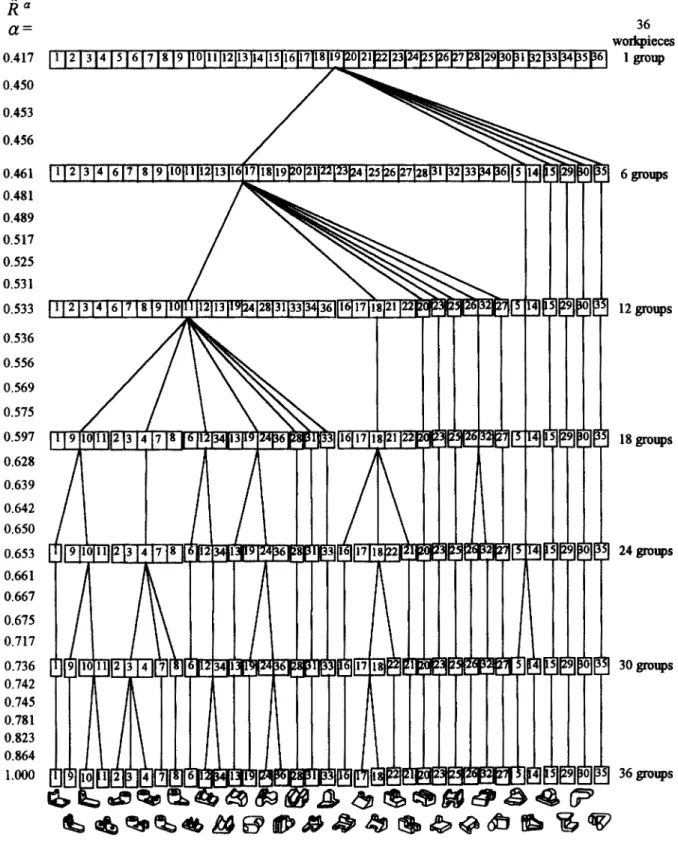
Consider an example of partial experimental data based on comparisons with eight typical workpieces (the 24th, 14th, llth, 1st, 26th, 18th, 3rd, and 12th workpieces in Fig. 2) collected from 30 subjects. In which each subject should make a total of 252 individual comparisons. Through the global shape similarity comparison of the typical workpieces with the other sample workpieces, the level of similarity among the 36 workpieces can be inferred by using the max-min method. Taking the inferred complete experimental data to calculate the max-min transitivity, we find that /)8 = / ) , and then this fuzzy relation is just a similarity relation on X. Taking the a- cuts (1, 0.864, 0.823, 0.781 . . . 0.417) in decreasing order of similarity, we find that different a-cuts of the membership matrix (/~) yield different numbers of groups in each hierarchy. An exhaustive list of the clustering results gives us the lean classification established by these eight typical workpieces (see Fig. 7).

To obtain the full-data classification, we had the 30 subjects classify the 36 sample workpieces and thus obtained actual complete experimental data from their pair similarity comparisons. The list of the results for different numbers of groups in each hierarchy is the full-data classification.

3. Measuring the Effectiveness and

Efficiency of Lean Classification

2.5.2 Establishing Lean Classifications for Different

Numbers of Typical Workpieces and Establishing

Full-Data Classification

By means of fuzzy clustering analysis, we can take the complete experimental data inferred by using comparisons between different numbers of typical workpieces and all the sample workpieces or the actual complete experimental data obtained from pair similarity comparisons of all the sample workpieces and use these data to formulate a classification. The level of similarity between the 36 sample workpieces can be regarded

~0.3

~

0.4 ~

0.5

a~0.8

~1

.0

Ix, lx3?,l

Fig. 6. Using fuzzy clustering for Example 1.

After establishing the lean classification and full-data classification, we can compare them to determine the degree of consistency between the two. We can then evaluate the effectiveness and efficiency of the lean classification, which is determined by its consistency with the full-data classification and the extent to which it reduces the cost of establishing a classification. These issues are discussed in the following sub- sections.

3.1 Consistency of the Lean Clauiflcstlon with the Full-Data Classification for the Same Groups

At present, no useful method is available for comparing the

degree

of consistency between two different classification sys-

tems applying different classification methods. Therefore, the aim of this section is to develop a heuristic algorithm for measuring the consistency between the classification results for the same groups in the lean classification and full-data classification. The idea is to take the classification results of full-data classification as a benchmark and calculate the ratio of the sum of the number of workpieces in each corresponding group in the two classifications that are the same over the total number of workpieces within each group. This ratio will be referred to as the degree of consistency between the lean classification and the full-data classification. The higher the

(8)

488 S. H. Hsu et al. R a Ot = 0.417 [ ' ~ 0.450 0.453 0.456 0.461 [ ~ 0.481 0.489 0.517 0.525 0.531 0.533 ~ 0.536 0.556 0.569 0.575 0.597 0.628 0.639 0.642 0.650 0.653 0.661 0.667 0.675 0.717 0.736 0.742 0.745 0.781 0.823 0.864 1.000

Fig. 7. Lean classification inferred from data for 8 typical workpieces by the max-min method. degree of consistency, the more consistent the two sets of

classification results are. Let the term corresponding groups refer to groups in the two classification schemes that have a one-to-one relation when the classifications have the same number of groups. The algorithm used for measuring the degree of consistency between two classifications is as follows:

36 workpieces 1 group 6 groups 12 groups 18 groups 24 groups 30 groups 36 groups

Step t: Arrange the two sets of classification results in a 2D matrix, with one set as a column and the other as a row 1. Suppose there are n workpieces, x~, x2 . . . x~, whose group

numbers are indicated by l, after being classified by the two classification methods, and the results are denoted by A~ . . . Ai . . . Al and BI . . . B i . . . Bt, respectively. Ai

(9)

refers to the set of workpieces within group i of the first classification. B~ refers to the set of workpieces within group j of the second classification.

2. Place the two classification results in columns or rows, respectively (see Table 1).

Table 1. Two sets of classification results arranged in 2D matrix.

1st 2nd classification classification B , . . . Bj . . . B, A~ cN . . . c~ i . . . c~t d~ A~ cim . . . c o • . . ca d~ At cll . . . c O . •. ctl dl

S t e p 2: Let C~j in the 2D matrix be the number of workpieces included in both At and B i, that is cij = N(A~ fq Bj)

S t e p 3: Determine the corresponding groups

1. Arrange all values of ctj in decreasing rank, i = 1,2 . . . l , j = 1,2 . . . I.

2. Take the largest value of clj. The At and B i corresponding to this cij will then be the first corresponding pair of groups from the two classification methods. Delete the row i and column j that correspond to this cti in the matrix.

3. If there are two or more identical largest values of ctj, then compare the second-largest value in the ith row and the jth column corresponding to these values o f ctj. Select the smaller of the second-largest values. If the second-largest values are also identical, then compare the third-largest values, and so on until a result is obtained. If the last values for comparison are still the same, then choose either. 4. Repeat the above three procedures for the undeleted values

of c 0 until all values of c~j have been deleted.

S t e p 4: Measure the degree of consistency between two classifications with I groups

1. Let di denote the value of cti for each pair of corresponding groups.

2. Let H denote the number of workpieces shared by all corresponding groups over the total number o f workpieces. The value of H is calculated as follows:

Efficient Benchmark Classifications 489

!

H - i=l (11)

n

H is the degree of consistency between two different classification schemes. The value of H falls between l l n and I. If there are a large number of workpieces, that is, n-> 0, then the value of H may fall between 0 and 1. Example 2 illustrates how H is found.

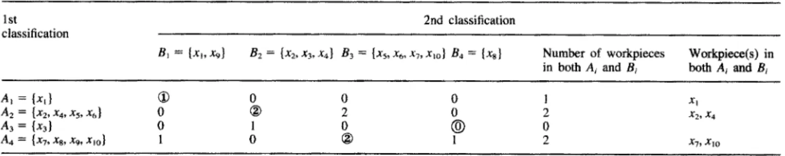
E x a m p l e 2. Consider a set of I0 sample workpieces (x~,x2 . . . X~o). Suppose two classification schemes each include four groups, as shown in Table 2. We will use the above algorithm to calculate the degree of consistency between the two sets of classification results.

First, we calculate the number of workpieces ctj that appear in any pair of groups Ai and Bj, as shown in Table 2. In this case, the value of c~ is 1, which means there is only one workpiece x~, that is included in both As and B~. Secondly, we arrange all values of c 0 in order from largest to smallest. The largest value is 2, and there are three sets, c22, c23, and c43 , with this value. So we then compare the second-largest value in each of the rows and columns corresponding to these three sets, and we find that in each case the second-largest value is 2. Hence, we must go on to compare the third-largest values in each row or column, which are 1, 2, and 1, respectively, and then compare the fourth-largest values between c22 and c43 , which are 0 and 1, respectively. Thus, for the first pair of corresponding groups we must choose A2 and B2 (c22), and so we delete the second row and the second column. Now we repeat the procedure and arrange all undeleted values of cij in order from largest to smallest. The largest value remaining is c43. Therefore, the second pair of corresponding groups is A4 and B3. We repeat this procedure until all the values of c o are deleted from the matrix. In this example, we eventually obtain four pairs of corresponding groups: A~ and B~, A2 and

B2, A 3 and B4, and A 4 and B3. The number of workpieces shared between each of these pairs of corresponding groups is 1, 2 , 0 , and 2, respectively. T h u s H = (1 + 2 + 0 + 2)/10 = 0.5, which is the degree of consistency between these two classification schemes when the number of groups is 4. 3.2 Evaluating the Effectiveness of Lean Classification

In both the lean classification and the full-data classification, users' judgements concerning the degree of similarity between

Table 2. The two sets of classification results in example 2.

1st 2nd classification

classification

B~ = {xj, xg} B2 = {x2, x3,x4} B3 = {xs, x6, xT, x~o} B4 = {x8} Number of workpieces Workpiece(s) in in both Ai and Bi both A~ and B~

A~ = {xt} 03 0 0 0 1 x~

A2 = {x2, x4, xs, x6} 0 ( ~ 2 0 2 x2, x4

A 3 = {Xa} 0 1 0 (~) 0

(10)

490 S. H. Hsu et aL

different workpieces can be employed to choose the number of groups used in the classification scheme. If the user requires that only workpieces with a very high degree of similarity be placed in the same group, then a higher a value can be used as the basis for the classification, and there will be more groups but fewer workpieces within each group. If the user can allow workpieces with a lower degree of similarity to be classified in the same group, then a lower et value can be used as the basis for the classification, and there will be fewer groups but more workpieces within each group.

The average degree of consistency of lean classification with different typical workpieces is evaluated with reference to the full-data classification result comprising different numbers o f groups of 36 workpieces. The average degree of consistency is plotted as shown in Fig. 8. In the case of the lean classification with eight typical workpieces, the average degree of consistency for every number of groups is 78%. In other words, the classification results based on only 40% (the partial experimental data with eight typical workpieces are 252 and the complete experimental data are 630) of the complete experimental data are 78% consistent with the results o f full- data classification.

4. Simulation Method for Evaluating the

Effectiveness and Efficiency of Lean

Classification

The example used in Section 3 to demonstrate the efficiency of lean classification included only 36 sample workpieces. To determine whether lean classification maintains a high level of efficiency even when a large number of sample workpieces are being classified, we will present in this section a simulation method for estimating the efficiency of lean classification for sets of from 100 to 800 sample workpieces. In Section 4.1, we construct a simulation matrix; in Section 4.2, we determine a reasonable interval o f degrees of similarity between two workpieces; and in Section 4.3 we simulate the efficiency of lean classification for a large number of workpieces.

4.1 Constructing a Simulation Matdx

To use a simulation method to evaluate the efficiency of lean classification, we need to construct a simulation matrix S. The elements in the matrix will denote the simulated degree of similarity as a subject performs pair comparisons of n workpieces (x~, x2 . . . xn). The elements o f the matrix are interrelated in certain ways. For example, if two workpieces are both very similar to a third one, then these two workpieces will have a high degree o f similarity. Therefore, the values of the elements in S cannot be assigned randomly, but must be assigned in light of the interrelations between the elements. For convenience, we will use the reflexive and symmetric properties of the matrix, that is, s~ = 1, s~j = s~, and consider only the upper part o f the data in our discussion.

X 1 X2 S = [S0"]nn = X 3 x~ xt X2 x3 ... xn 1 6 ' 1 2 6 ' 1 3

"'" Sin

1 s23 .-* 6`2,, 1 ... s3, "... 1

(12)

The values of the elements in the simulation matrix are pro- duced as follows.

Step 1: Assign preliminary values to the first row.

Assign random numbers [0, 1] to the first row of the matrix su, j = 2 . . . n; this means the degree of similarity between workpiece xt and other workpieces (x2, x3 . . . x~) is known.

Step 2: Determine a reasonable interval among other rows sij. From the degree of similarity between workpiece x~ and other workpieces, a reasonable interval of degrees of similarity between any two workpieces, except those in the first row, can be inferred; that is, we infer the interval that sij, i = 2, 3 . . . n and j = i + 1 . . . n may fall in.

Step 3: Assign sli a value in the interval determined in step 2. Randomly assign si i a value in the interval of degrees of similarity between any two workpieces; this kind of simulation matrix will reflect that all the workpieces are interrelated in certain ways.

1 ~ o 9 0 o.91 o.94 o,96 O.78 0.1! -% 0,62

2~4°~'~

~

eor~lntcdamtn~l

Nu~oct

of

w f i t i i i i i i . . . . ]34 ~gs as2 305 354 ~,~ 4¢0 4"nstoS:'sc~s602630

O) (4) (6) (I) {to) (1~) (1t,) (16) Us) (20)(*~) 06) 06 ) ~ . . ~ ( .Humor o f

wontpm~ ) Fig. 8. Average degree of consistency for lean classifications with

different numbers of groups.

4.2 Determining Interval of Degrees of Similarity Between Two Workpleces

In constructing the simulation matrix, we need to know the degree of similarity between workpiece Xl and other workpieces in order to infer a general interval for the degree of similarity between any two workpieces (except for the first row of elements in the matrix). The theoretical basis o f the inference is to regard the information content of the global shape of each workpiece as a set. The total value is assumed to be 100%, that is, 1. The degree of similarity between the global shapes of two workpieces is then just the intersection of two sets. The inference method is to use the intersection o f the sets representing the global shape information o f any two

(11)

workpieces and workpiece xt to determine the smallest and largest possible intersection between the two workpieces. These will then serve as the lower bound and upper bound o f the interval o f the degree of similarity between the two workpieces. Take two workpieces xp and xq as an example. Let s m Sq

and s~ denote the global shape information o f the three workpieces x m Xq, and xt, respectively. Assume that the degree of similarity between xp and xt is spt and that between xt and Xq

is Stq, and we want to find a reasonable interval of the degree of similarity between the two workpieces xp and Xq. First, we find the lower bound of the interval of s m by finding the smallest intersection between sp, Sq and sj. See Fig. 9(a). When sp and sq are on different sides of s~, then spt = sp fq st and

stq = st f3 Sq; when spt + Stq > 1, the lower bound of s m is

spj + S~q - 1; and when sp~ + Stq -< 1, the lower bound of S,q

equals 0. Secondly, to calculate the upper bound of the interval of s m we find the largest intersection set between sp, Sq and

sj see Fig. 9(b). Now Sp and Sq are both on the same side of st. When spl -- stq, the upper bound of s m is Spt + (1 - Stq);

when spt >-- S~q, the upper bound is Stq + (I - SpO. These two formulae can be combined into the general formula

1 - I s p ~ - S q t ] . Thus, a reasonable interval for the degree of similarity between any two workpieces through x~ is [max [0, spt + SIq -- 1], 1 - ]sp~ - s~q]]. In the following section, we use Example 3 to illustrate this inference method.

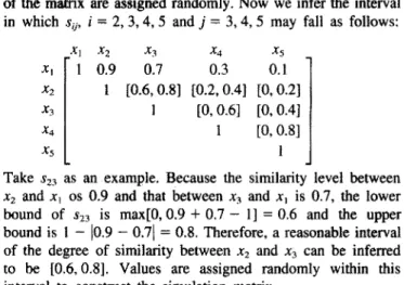
Example 3. Construct

a 5 × 5

simulation matrix. The preliminary values sv, j = 2, 3, 4, 5 of the elements in the first row

(a) Sl ]

N?

when spl + Stq > 1,

I

of the matrix are assigned randomly. Now we infer the interval in which s~j, i = 2, 3, 4, 5 and j = 3, 4, 5 may fall as follows:

xi x2 x3 x4 x5 xt 1 0.9 0.7 0.3 0.1 x2 1 [0.6, 0.81 [0.2, 0.4] [0, 0.21 x3 1 [0, 0.6] [0, 0.4] .,c4 1

[0,

0.81

x5 1

Take sz3 as an example. Because the similarity level between Xz and x~ os 0.9 and that between x3 and xt is 0.7, the lower bound of s~3 is max[0,0.9 + 0 . 7 - 1] = 0.6 and the upper bound is 1 - [0.9 -

0.71

= 0.8. Therefore, a reasonable interval of the degree o f similarity between x2 and x3 can be inferred to be [0.6, 0.8]. Values are assigned randomly within this interval to construct the simulation matrix.

4.3 Using a Large Sample to Examine the Efficiency of Lean Classification

Once the simulation matrix has been constructed, we can formulate a simulated full-data classification on the basis of all the data in the matrix. We can also take a portion of the data and use the max-min method to infer classification results for the complete data, thus obtaining a simulated lean classification. By measuring the consistency between the two classification results and comparing the cost of establishing the lean

t St ] ... s ~ = ~

when Sp, +

Slq < 1, Spq = 0 (b) I" 1 ~l s, [ !i

s.

I

when spl <

Stq , Spq = Spl + (1 - Stq ) .

St

'

'["

[

s,, j

s, ~ "!

when

spt >_ Stq , $pq = slq + (1 - Spl ) .

:.s,q= l - t , , , - , d

I

(12)

492 S. H. Hsu et al.

classification and full-data classification, we can determine the efficiency of the simulated lean classification. As it is very difficult to judge the global shapes of n sample workpieces from the simulation matrix, the typical workpieces used in the simulated lean classification are selected, not by the binary clustering method described in Section 2, but, directly from the n sample workpieces by their order, based on the required number of typical workpieces. For instance, to establish a simulated lean classification base on six typical workpieces, we can take the first six rows o f elements directly from the simulation matrix as partial experimental data.

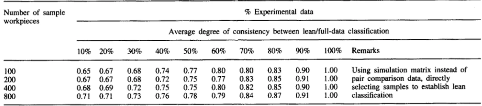
To examine the efficiency of the lean classification method, we constructed four simulation matrixes, with 100, 200, 400, and 800 sample workpieces, respectively. The values of the elements were set to the second decimal place, and then lean classification was simulated with different typical workpieces. To compare the classification results for these four sets of sample workpieces, we will use lean classifications employing from 10% to 100% of the complete experimental data to calculate the average degree of consistency with the full-data classification for different numbers of groups (see Table 3).

From Table 3 we can make three interesting observations. First, the results of lean classification based on only a small portion of the data are still highly consistent with the results of full-data classification. For example, for 800 sample workpieces, the degree of consistency between the lean classification based on only 10% of the complete data and the full-data classification was 71%. Secondly, when the percentage of the experimental data used in formulating the lean classification is doubled, only a limited increase occurs in the degree of consistency with the full-data classification. For instance, suppose there are 800 sample workpieces. If the percentage of the experimental data used is increased fivefold, that is, if a lean classification is established with 50% of the complete data, then the degree of consistency between the lean and full- data classifications will be 78%, an increase of only 7%. Moreover, the size of this increase continues to shrink as the amount of data used in the lean classification increases. Thirdly, as the number of sample workpieces increases, a lean classification using the same percentage of the data achieves an increasing degree of consistency with the full-data classification. For example, suppose the number of sample workpieces increases from 100 to 800. Then the degree of consistency between the full-data classification and a lean classification based on just 10% of the complete experimental data increases from 65% to 71%.

These simulation results show that in a practical workpiece classification application, as the number of sample workpieces increases, only a small portion of the complete experimental data is needed to produce a lean classification that is highly consistent with the full-data classification. For a sample of 800 workpieces, for example, gathering complete experimental data would involve making 319600 pair comparisons. However, if lean classification were used instead, we could produce a classification that was 71% consistent with the full-data classification while using just 40 typical workpieces (less than 10% o f the total data) and making only 31 180 pair comparisons.

5. Application and Limitations of Lean

Classification

When full-data classification is employed as a benchmark to measure the performance of an automatic classification system, the automatic classification system under test and the full-data classification are both used to classify the same group of sample workpieces, and then the degree of consistency between their results is compared. In this paper, we have described a type of lean classification, which enables us to establish a benchmark on the basis of only a small percentage of the experimental data needed to establish a full-data classification. The simulation method described above allows us to determine the degree of consistency between a lean classification and a full-data classification for different numbers of typical workpieces. Selecting an appropriate lean classification to measure the performance of an automatic classification system enables us to evaluate the performance o f the automatic classification system, just as if we were using a full-data classification. Since only a lean classification is used, however, such a comparison is much more efficient.

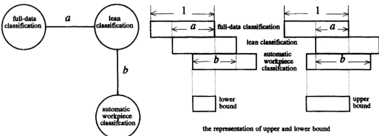
The method for employing a lean classification to evaluate the performance of an automatic classification system is an extension of the method described in Section 4.2. In Fig. 10, for example, let a represent the degree of consistency between the lean classification and the full-data classification, and let b represent the degree of consistency between the results of the automatic classification system and those of the lean classification. The term b can also be regarded as representing the performance of the automatic classification system as measured by the lean classification. Denote the value of an interval by

[x,y], in which the lower bound x = max [0, a + b - 1] and the upper bound y = [1 - la - bl]. For example, if the degree

Table 3. Degree of consistency between lean and full-data classifications for samples of 100 to 800 workpieces.

Number of sample % Experimental data

workpieces

Average degree of consistency between lean/full-data classification 10% 20% 30% 40% 50% 60% 70% 80% 90% 1 0 0 % Remarks

100 0.65 0.67 0.68 0.74 0.77 0.80 0.80 0.83 0.90 1.00 Using simulation matrix instead of 200 0.67 0.67 0.68 0.72 0.75 0.77 0.83 0.85 0.91 1.00 pair comparison data, directly 400 0.68 0.69 0.72 0.75 0.75 0.80 0.82 0.85 0.90 1.00 selecting samples to establish lean 800 0.71 0.71 0.73 0.76 0.78 0.79 0.84 0.87 0.91 1.00 classification

(13)

f

i

Fig. 10. Using lean classification to evaluate the performance of an

aJ .

_q

L

b

>i

I"

' - - ~ lower bound

L

elassigcalion ~,, lean ¢lassilication i,

_I'

]

11

upper

the representation of upper and lower bound

automatic classification system with respect to full data classification. of consistency between the lean classification and the full-data

classification is 0.71, and that between the results of the automatic classification and those o f the lean classification is 0.9, then we can infer that the degree of consistency between the automatic classification system and the full-data classification should fall in the interval [0.61, 0.81]. If the degree of consistency between the lean classification and the full-data classification is reduced to 0.4 and that between the results of the automatic classification system and those of the lean classification is still 0,9, then the degree of consistency between the automatic classification system and the full-data classification is within [0.3, 0.5]. This interval gives us an estimate of the performance of the automatic classification system measured with respect to the full-data classification.

By using such intervals to estimate the performance of an automatic classification system with respect to the full-data classification, we can investigate the application and limitations of lean classification. As shown in Fig. 10, if we want to find a useful automatic classification system that is compatible with users' judgements of the similarity between workpieces, two conditions have to be satisfied. First, there must be a high degree of consistency between the lean classification selected and the full-data classification - the degree of consistency must at least fall within the scope of tolerance of the user. Secondly, the performance of the automatic classification system as measured by the lean classification must be high. In this case, the lean classification can just replace the full-data classification as the classification benchmark used to select an optimal automatic classification system. Consider again the above example. Suppose a = 0.71, a value that is within the scope of tolerance of the user, and b = 0.9. Then the performance of the automatic classification system as measured by the full- data classification falls in the interval [0.61, 0.81]. If the users find values in this estimated interval acceptable, then they may decide to adopt the automatic classification system under test. This is a typical way in which lean classification could be used to replace full-data classification. However, when a has a lower value, we will be unable to use the lean classification to identify an automatic classification system compatible with users' judgements. In that case, we would have to use the full- data classification as a benchmark; this is the main limitation of lean classification in practical applications. Let us look again

at the above example. If a = 0.4 and b = 0.9, the performance of the automatic classification system with respect to the full- data classification can he estimated by the lean classification as falling in the interval [0.3, 0.5]. Because values in this interval are very low, in this case users would not want to accept the test classification system for practical use. Hence, in this case, the lean classification would not he useful for identifying an optimal classification system but instead would only be useful for sifting out ineffective automatic classification systems.

6. Conclusion

To evaluate the performance of an automatic classification system, we need to examine whether its classification results are consistent with users' judgements. The higher the degree of consistency, the more effective the classification, Therefore, classification benchmarks based on users' judgements are necessary. Such a benchmark is typically established by having a large number of subjects make exhaustive pair comparisons between all workpieces in a group of sample workpieces and then using their judgements to classify the workpieces. A classification based on this type o f exhaustive data is called a full-data classification. A full-data classification provides an accurate evaluation of the performance o f an automatic classification system, but when a large number of samples are involved, it may be costly, time-consuming, and unreliable because of bias due to fatigue among the subjects.

To mitigate these shortcomings, this paper has proposed a lean classification method, in which only a relatively small number of typical workpieces are used to make pair comparisons with all of the sample workpieces. The partial experimental data are then used to infer results similar to those that would be obtained from the complete experimental data. In an experiment with a small set of 36 sample workpieces, if we take eight typical workpieces which in turn represent only 40% of the complete experimental data, the average degree of consistency between the classification results for various numbers of classification groups, the lean classification is 78% consistent with the full-data classification. In simulations with medium to large samples of 100 to 800 workpieces, we found

(14)

494 S. H. Hsu et al.

that when the number of workpieces increases, if we take the average degree of consistency of the classification results for various numbers of groups, a lean classification established with only 10% o f the complete experimental data is 71% consistent with the full-data classification.

We can also use lean classification to evaluate the performance of automatic classification systems measured with respect to full-data classification. However, lean classification can be used to select an effective automatic classification system only when the degree o f consistency between the lean classification and the full-data classification is within the user's scope of tolerance and that the automatic classification system achieves a high level of performance as measured by the lean classification. If one or both of these two conditions fails to be satisfied, then the lean classification can be used only as a tool for sifting out inferior classification systems, and not for selecting an effective system.

Acknowledgement

The authors thank the employees o f the Aircraft Manufactory, Aerospace Industrial Development Corporation (AIDC), Taichung, Taiwan, for their participation in the workpiece pair comparison experiment.

References

1. A. Bhadra and G. W. Fischer, "A new GT classification approach: a data base with graphical dimensions", Manufacturing Review, 11, pp. 44 49, 1988.

2. C. S. Chen, "A form feature oriented coding scheme", Computers and Industrial Engineering, 17, pp. 227-233, 1989.

3. M. R. Henderson and S. Musti, "Automated group technology part coding from a three-dimensional CAD data-base", Transactions of the ASME Journal of Engineering for Industry, 110, pp. 278- 287, 1988.

4. S. Kaparthi and N. Suresh, "A neural network system for shape- based classification and coding of rotational parts", International Journal of Production Research, 29, pp. 1771-1784, 1991. 5. T. Lenau and L. Mu, "Features in integrated modeling of products

and their production", International Journal of Computer Integrated Manufacturing, 6(1 and 2), pp. 65-73, 1993.

6. M. C. Wu, J. R, Chen and S. R. Jen, "Global shape information modeling and classification of 2D workpieces", International Jour- nal of Computer Integrated Manufacturing, 7(5), pp. 216-275, 1994.

7. M. C. Wu and S. R. Jen, "A neural network approach to the classification of 3D prismatic parts", International Journal of Advanced Manufacturing Technology, 1t, pp. 325-335, 1996. 8. S. H. Hsu, T. C. Hsia and M. C. Wu, "A flexible classification

method for evaluating the utility of automated workpiece classification system", International Journal of Advanced Manufacturing Technology, 13, pp. 637-648, 1997.

9. S. K. Thompson, Sampling, John Wiley, New York, 1992. 10. W. Labov, "The boundaries of words and their meanings", in

C.-J. N. Bailey and R. W. Shuy (eds) New Ways of Analyzing Variations in English, Washington, DC: Georgetown University Press, 1973.

11. S. J. Chert and C. L. Hwang, Fuzzy Multiple Attribute Decision Making - Method and Application, A State-of-art Survey, Springer-Verlag, New York, 1992.

12. H. Bandemer and W. Nather, Fuzzy Data Analysis, Kluwer Aca- demic Publishers, 1992.

13. F. Bouslama and A. Ichikawa, "Fuzzy control rules and their natural control laws", Fuzzy Sets and Systems, 48, pp. 65-86, 1992.

14. H. J. Zimmermann, Fuzzy Set Theory: and Its Application, 2nd edn, Klnwer Academic Publishers, 1991.

15. S. K. Tan, H. H. Teh and P. Z. Wang, "Sequential representation of fuzzy similarity relations", Fuzzy Sets and Systems, 67, pp. 181-189, 1994.

16. G. J. Klir and T. A. Folger, Fuzzy Set, Uncertainty, and Infor- mation, Prentice-Halt, 1992.