Efficiency and Reliability in Cluster Based
Peer-to-Peer Systems
CHING-WEI HUANGAND WUU YANG Department of Computer Science
National Chiao Tung University Hsinchu, 300 Taiwan E-mail: rollaned@gmail.com E-mail: wuuyang@cs.nctu.edu.tw
Peer-to-peer systems have become one of the most popular Internet applications. Some unstructured systems such Gnutella perform file searching by flooding requests among nodes. It has been proven that such unstructured systems are not scalable, and searching consumes tremendous bandwidth. We propose three mechanisms to recon-struct the system topology and improve message flooding. Our research addresses four aspects: system topology control, message routing, message locality, and system con-nectedness. The simulation shows that significant redundancy in flooding of messages can be eliminated and message locality achieves a high ratio.
Keywords: peer-to-peer system, cluster, Gnutella, message routing, distributed system
1. INTRODUCTION
Since the music sharing software Napster appeared in 1999, peer-to-peer file sharing services have become very popular. The P2P model brings new solutions to solve the bottleneck in the traditional client-server model. Besides the file sharing service, other traditional network services such as web browsing, instant messaging, or media stream-ing now may use the P2P model to improve their performance and efficiency.
However, the P2P model is not perfect; some inherent weaknesses of the P2P model should be addressed before it is applied. HOPs servers, the communication in P2P sys-tems, depend on message delivery between nodes or message flooding among nodes. The later consumes bandwidth extremely. On the other hand, a P2P system is maintained by each node in a distributed way. In other words, the system must be self-organized. Each node in the system cooperates with each other to make communication efficient and re-cover the system if failures occur. A poorly designed P2P system may result in huge maintenance costs.
In the following paragraphs, we introduce three issues that our research addresses. System Topology Control The network topology significantly affects the performance of a P2P system. One obvious example is the Gnutella network, one of the most famous P2P systems. Recent research [1] shows that the message routing protocol of Gnutella generates a huge number of redundant message. The number of messages originating from one request in the Gnutella network is estimated to be
0
2∗
∑
TTLi= C∗(C−1) ,i whereC is the average number of neighbors per node and TTL is the average number of HOPs of each message. We assign the value of TTL to be 7, which is the average number of HOPs for requests according to [5]. If the average number of neighbors per node is 4, the estimated number of messages originating from one request is 26,240. If the aver-age number of neighbors per node is 8, the estimated number of messaver-ages rises to 15,372,800.
On the other hand, the Internet is a collection of autonomous systems connected by routers. An autonomous system (AS) [5, 13] is a set of routers under a single technical administration that uses an interior gateway protocol and common metrics to route pack-ets within the AS and an exterior gateway protocol to route packpack-ets to other AS’s. If the messages travel across different AS’s frequently, the communication will be prohibitively expensive. The research shows that only 2 to 5 percent of connections in Gnutella are within a single AS.
A plausible cause of these problems is that Gnutella does not control system topol-ogy. Arbitrary connections will result in massive redundant messages. An appropriate system topology, such as a tree, may provide efficient message delivery and hence re-duces the number of redundant messages. However, additional messages are required to maintain the appropriate topology of the system.
Message Routing Message routing plays a key role in a P2P system. In order to ana-lyze the performance of message delivery in P2P systems, three measurements are com-monly used: the average number of HOPs for requests, the clustering coefficient of the system topology [2, 3], and the number of flooding messages originating from one re-quest. For the HOPs of requests, the fewer the average number of HOPs, the lower the communication cost. For the clustering coefficient, the higher the clustering coefficient of a graph, the more nodes are connected in a regular fashion. The lower the clustering coefficient of a graph, the more nodes are connected randomly [3]. Paper [3] also shows that a small-world network could have the benefits of both a higher clustering coefficient and a lower average number of HOPs.
In a P2P system, a search request travels through nodes by successive message broadcasts on each node. Redundant broadcast messages may consume a major part of the network bandwidth if there is no control on the message routing. We propose a mes-sage routing mechanism which reduces the number of redundant mesmes-sages originating from one request.
System Connectedness The last issue that we discuss is the connectedness of the P2P system. Due to possible disconnections between nodes such as leavings or failures of nodes, a P2P system could possibly be split into disconnected components. A split system leads to poor search performance because requests may not reach enough nodes. For a dynamic system, it is necessary to tolerate splitting of the system. And, the system should be able to recover failures and re-connect components.
In this paper, we present DSE (Distributed Search Environment), our P2P system. DSE concentrates on the above three aspects and proposes solutions to the respective problems. The rest of this paper is organized as follows. Section 2 illustrates the archi-tecture of DSE systems and our simulation methodology. Section 3 introduces the
mechanism to control the system topology. Section 4 introduces an efficient message routing mechanism which is based on the cluster structure of the system. Section 5 shows the recovery mechanism to handle splits of the system. Section 7concludes this paper.
2. SYSTEM ARCHITECTURE AND SIMULATION
2.1 System Architecture
The DSE system runs on each node and contain three major mechanisms: neighbor clustering control (NCC), smart message routing (SMR), and ring-around-leader (RAL). The NCC mechanism controls system topology by selecting neighbors of each node. The SMR mechanism controls the routing path of each message. The RAL mechanism detects and reconnects split components of the system if they exist. Fig. 1 (a) shows these mechanisms and corresponding data structures.
Originator NID NCC SMR RAL Originator Address DSE System Data Structure Functions Message Neighbor List CID / NID MTAG Buf MTAG BCTL Originator CID Data (a) (b) Fig. 1. Three mechanisms of the DSE system and message structure.
2.2 Simulation Methodology
To verify the performance of the DSE system, we adopt a strategy of developing both a real system and a simulator. The real system, with a project name Apia is publicly available[15]. Currently there are more than 40,000 registers and 1,000 to 2,000 online users. We collect user-related data such as host addresses, search requests, online time,
etc., for the simulator to verify NCC, SMR, RAL mechanisms and other related
im-provements. In one week of tracking, we captured 5,718 users and selected 1,692 of them who stay online the largest amount of time. To simplify our simulations, conditions of dynamic and multiple IP address binding are not considered. The distribution of ad-dresses of these nodes is listed in Table 1, which shows that most of them come from the major ISPs of Taiwan. During the tracking period, we collected 200,198 search requests which originated from these nodes.
In the following sections, the simulator builds a system with 1,000 to 2,000 nodes; each node performs the NCC, SMR, and RAL tasks simultaneously and continuously. Each node generates a search request every 20 to 60 seconds.
Table 1. ISP distribution of nodes and message locality.
ISP HINET TANET SEEDNET APOL GIGA SONET OTHERS
Node Number 547 436 196 152 115 61 185
Percentage 32.33% 25.77% 11.58% 8.98% 6.80% 3.61% 10.93% Message Locality 79.00% 76.72% 63.45% 66.97% 66.02% 64.33% N/A
Our simulation analyzes the NCC, SMR and RAL mechanisms in the following as-pects: the average number of flooding messages generated by one request (called AMOR), the average number of HOPs of request (called HOPOR), the clustering coeffi-cient, reduced messages when SMR is enabled, and the relation between AMOR and dynamic behaviors of nodes.
3. NEIGHBOR CLUSTERING CONTROL
NCC mechanism has two goals: (a) promote message locality and (b) reduce re-dundant flooding messages and lower the number of HOPs of search requests. To achieve the first goal, the NCC mechanism introduces a new address format called HIP which considers IP distribution of ISPs (more precisely, the AS structure of the Internet) for better connections. With a clustering structure of the system, most flooding messages travel within their ISPs. Hence, the communication cost of message flooding can be re-duced. To achieve the second goal, the NCC mechanism introduces a notion of node dis-tance based on which nodes are organized into connected clusters so that the characteris-tic path length is shorter and the clustering coefficient remains high [3]. By cooperating with the SMR mechanism, redundant messages in message flooding can be reduced.
3.1 Node Cloning
When a new node joins the system, the DSE system initially asks the user to input some arbitrary sentences. The speed of typing and the sentences are treated as user be-havior related information. The DSE system then generates a unique ID, called NID, for the node using the SHA1 function, with an argument which contains the IP address of the host, a standard time stamp, and the user behavior related information. Consider the ex-ample in Fig. 2 (b) where a new node H1 sets up the argument for SHA1 when it joins the system. H1 : 868C6DDD03 H2 : 71DC0E4E5D H3 : 868C710101 H4 : 868C751D64 H5 : 868C6EFA7D H6 : 868C6D1E09 H2 H1 H3 H4 H6 H5 H0 by H4 by H3 by H0 by H4 IP ADDRESS : 140.109.221.3
TYPING SPEED : 30 CHARS/SEC HIP ADDRESS : 868C6DDD03 INPUT SENTENCE : Hi, I come from Orion TIMESTAMP : 1095233434.3698 IP
H0 : 3C96142B0B
(a) (b) Fig. 2. A newly joining node and neighbor updating.
The argument fed to SHA1 varies the NID of each node. For any two given nodes
Ha and Hb, DSE system generates the same NID if all of the following conditions hold:
Ha and Hb join the system at exactly the same time, both of them join the system with the same IP address; and both of them generate the same user behavior related information. Obviously, it is almost impossible for any two new nodes to obtain the same NID. The uniqueness and comparability of each NID are necessary for the NCC mechanism to con-trol node connections, and the SMR mechanism to reduce redundant messages in mes-sage flooding.
Since there are no servers to provide a list of initial neighbors for each new node to connect to, the DSE system chooses some default nodes, called navigators, to serve as the initial neighbors for every new node. Navigators perform exactly the same as other nodes except that all new nodes initially connect to them. The addresses of navigators can be resolved by DNS. Therefore, navigators need not be some fixed hosts. Through dynamic mapping of domain names and IP addresses, every node in the system can be a navigator. Once a new node connects to any one of the navigators, it successfully joins the system and begins to find more neighbors. In the following sections, we allocate five navigators for the system in each simulation.
Standard global time is important for data synchronization among nodes in the sys-tem. Each node reads the current standard global time by periodically querying the net-work time servers with Netnet-work Time Protocol (NTP) [12]. The RAL mechanism (dis-cussed in section 5) uses standard time and message exchange between nodes to detect whether the system is split.
Although each node in the DSE system synchronizes its local time to standard global time, the scalability of the system will not be limited because of the following reasons: (a) plenty of NTP servers on the Internet are available to provide NTP service; (b) synchronization with standard global time needs to be performed only every few hours; (c) neighbors can synchronize standard global time with each other if any one of them synchronized it from any NTP server.
3.2 Node Clustering 3.2.1 Basic notion
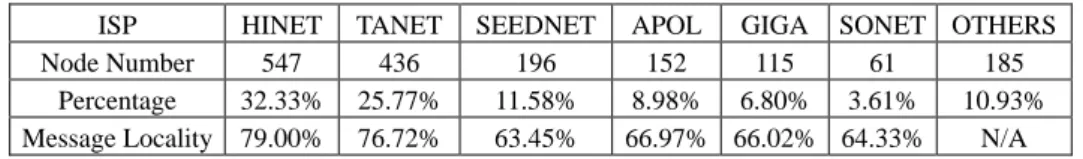
Instead of controlling node connections based on traditional IP address format (x.y.z.w), we adopt a new address format called HIP. The HIP format is composed of two parts. For the first part, we give each ISP a unique identifier, called ISPID, in two hexa-decimal characters form. The second part of HIP is an eight hexahexa-decimal characters form of the original IP address. Fig. 3 (a) shows the HIP of a given host. The ISPID is 4C
which represents the ISP identifier that the host belongs to. The rest of HIP, 8C6DFA70, is the 8-hexadecimal character representation of the IP address 140.109.250.112.
Before using HIP to control node connections, we give some related definitions. First, we define the depth of each character in HIP as its position in HIP (started from 0). Second, we define the prefix of HIP of size K, denoted by Prefix(HIP, K), as the sub-string of the first K + 1 characters. Third, the (K + 1)’th character of HIP is denoted by
depthChar(HIP, K). Fig. 3 (a) shows each depth of a given HIP and Prefix(HIP, 6). For a given character C in the circle of hexadecimal characters (0-9, A-F), we define the left
E IP = 140.109.250.112 HIP = 4 C 8 C 6 D F A 7 0 IP ADDRESS (depth 2 to 9) ISPID (depth 0,1) Prefix(NID,6) = 4C8C6D left side right side cycleDistance(3,E)=5 0 1 2 3 4 F D B A 0 9 8 7 6 5 C (a) (b) Fig. 3. HIP prefix and the left/right side of character “2”.
side of C as the anti-clockwise half characters by C, and the right side of C as the clock-wise half characters by C. And cycleDist(A, B) is defined as the length of the shortest path between characters ‘A’ and ‘B’ on the circle of hexadecimal characters. Fig. 3 (b) shows the circle, left/right sides of character ‘2’, and cycleDist(3, E).
On the other hand, for a given node X, we define node Y as a left/right neighbor of node X in depth K if depthChar(Y, K) is in the left/right side of depthChar(X, K), and
Prefix(HIPy, K − 1) = Prefix(HIPx, K − 1) for K > 1 or depthChar(HIPy, 0) = depthChar
(HIPx, 0) for K = 0. For HIPs, the space at depth 0 is divided into 16 segments. HIPs Di with different depthChar(Di, 0) fall in different segments of depth 0. HIPs Di with the same depthChar(Di, 0) but different depthChar(Di, 1) fall in the same segment of depth 0 but in a different segment of depth 1. As a consequence, different HIP falls in a different position without collisions. Here we called such a distribution space of HIP the HIP space. The capacity of HIP space is 1610 because each HIP is a 10 character hexadecimal string. Such HIP space should be large enough to cover HIPs of billions of nodes.
3.2.2 Connection rules
The connections of nodes are determined based on two rules: near-first and depth- first. The near-first rule makes nodes connect to each other to form hierarchical clusters. The depth-first rule controls connections across clusters so that these connections play roles of shortcuts for faster message travelling.
For the near-first rule, we introduce a notion called node distance which is based on which closer nodes connect to each other. Hence, the system structure is transformed to be hierarchical and connected clusters. Fig. 4 shows the definition of node distance. The node distance takes two HIP addresses to compute their distance. Each node continu-ously checks each new node that it meets. If the new one is nearer than its current neighbor, the current one will be replaced by the new one. We call these neighbors which are decided by the near-first rule the near-first neighbors.
9 (9 ) 0 distance( , ) cycleDistance( , )i i i i A B a b K − = =
∑
∗ A = a0.a1 … a9, B = b0.b1 … b9, K = 16Notice that the definition of node distance does not have to reflect the accurate dis-tance of the physical link between two nodes. The definition intends only to have nodes in the same AS connect to each other so that message locality (discussed in section 3.4) can be promoted and the SMR mechanism (discussed in section 4) reduces redundant flooding messages.
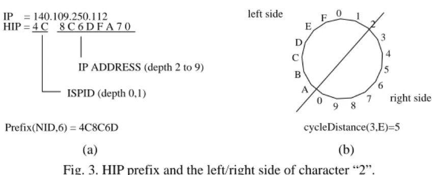
For the depth-first rule, each node tries to connect at least one left and right neighbor in every depth if they are available. Moreover, selected neighbors at each depth should be as near to the local node as possible. Consider the example in Fig. 5 where node H0 connects to its left and right neighbors at some depths. Node H0 made
connec-tions to H1 and H2 because they are right and left neighbors of H0 at depth 8. Similarly,
H4 is a left neighbor at depth 1 and H5 is a right neighbor of node H0 at depth 0. Notice
that it is not necessary that left and right neighbors at each depth are always available. When the system contains fewer nodes, the number of neighbors at more depths will be absent. On the other hand, since each node connects at least one left and one right neighbor at every depth (if they are available) and the HIP address has 10 depths, each node has at most 20 such neighbors. We called those neighbors which are decided by the depth-first rule the depth-first neighbors.
depth 9 H2 H1 H3 H4 H0 H8 H6 H5 H7 3 2 7 8 depth 0 H8 H7 H6 H5 H4 H3 H2 3843E7B933 9 3843E7B930 9 280879060A 0 765439F4EC 0 35AEF34273 1 7 8 R L L R L R L H0 N/A N/A H1 R 8 3843E7B987 3843E7B932 (67.231.185.1) 3843E7B902 3843E7BE46 L/R Depth NID
Neighbor (with repectto H0)
0 1 2 3
Fig. 5. Node connections.
In order to determine the correct HIP address of a given IP address, each node maintains an ISPID table to retrieve the ISPID of any given IP address. Since the AS structure of the Internet is not always fixed, the ISPID table should be able to be updated to reflect the current mapping of IP address ranges and their ISPIDs. DSE implements an ISPID table updating mechanism via message flooding. The designer or manager of DSE maintains the correct ISPID table on a regular time schedule and distributes it to all nodes to update their ISPID table via message flooding. Notice that the IP address ranges of ISPs are usually available to the public. For example, the IP address ranges of ISPs to be used in our simulation can be obtained from [20].
3.2.3 Forwarding path
Given a system G running the NCC mechanism, the forwarding path of messages determines how many HOPs, on average, a request takes to travel to every node. Since the travelling of each request is bread-first-search, the length of the shortest path from the request originator to other nodes determines the HOPs of the request.
Ha 2430992E87 Hk1 Ha Hk2 k3 H Hkt Hb 1 HOP 1 HOP Hb 8451320EFA Hk1 343A98BC46 Hk2 88C12D0675 Hk3 84186C1A61 Hkt 8451320E79 NODE HIP
Fig. 6. Forward path of a request from node Ha to node Hb.
Suppose the connections of system G are stable, the example in Fig. 6 shows how a given request R moves from a given node Ha to node Hb through the shortest path
be-tween them. First, Ha forwards R to its right neighbor Hk1 at depth 0. Then, Hk1 moves R
to it right neighbor at depth 0. Request R is forwarded continuously to right nodes at depth 0 until it arrives at node Hk2, where Prefix(HIPHk2, 0) = Prefix(HIPHb, 0). Since
depthChar(Hk2, 1) = 8 and depthChar(Hb, 1) = 4, the request R is forwarded by Hk2 to its
left neighbor at depth 1. The forwarding of R to left neighbors at depth 1 continues until it arrives at a node Hk3, where Prefix(HIPHk3, 1) = Prefix(HIPHb, 1). The following
for-warding of R continues until R arrives at node Hkt so that Prefix(HIPHkt, 8) = Prefix(HIPHb,
8). Then, Hkt moves R to its neighbor Hb.
Except for the first forwarding of R by Ha to its right neighbor at depth 0 (only takes
1 HOP), each time R is forwarded from one node to another at the same depth, it takes at most 8 HOPs (the cycleDist of any two nodes). Therefore, the upper limit of HOPs in the whole forwarding process of R to any node is 1 + 8 * 10. In a real system, the forwarding of a request takes much fewer than 81 HOPs because there are not that many nodes in the whole HIP space. For a system with N nodes, the number of forwarding between depths is log16N. Hence, the upper bound of HOPs in the whole forwarding process of a request
is 1 + 8 * log16N, or in general, O(log16N).
Notice that the connections to nodes at different depths play the roles of shortcuts between clusters to make the travelling of each request over the whole system faster. If each node maintains more distant neighbors (currently, two neighbors) at each depth, the upper bound of HOPs of each request will be less than O(log16N).
3.3 Neighbor Updating
In DSE, each node uses two methods to contact new neighbors: message recognition and neighbor introduction. The first method is fulfilled by message flooding. Consider the message structure shown in Fig. 1 (b). The header of each message records the IP address and NID of the message originator. When a node originates a flooding message, every node which received the message extracts the header and builds a connection to the
originator if it will be a better neighbor than its current neighbors (by node connection rules in section 3.2.2).
The second method introduces the use of third party neighbors. Each node periodi-cally gathers a set of NIDs and addresses of its neighbors, then broadcasts the set to its neighbors. Each neighbor who receives the set builds connections to some nodes in the set if they are better neighbors than current neighbors. Given nodes Hx, Hy, and Hz, we
say that Hx is introduced to Hy (or Hy is introduced to Hx) by Hz if the connection between
Hx and Hy is built via the neighbor set broadcasted by node Hz. Consider the example in
Fig. 2 (a), where a connection between nodes H1 and H6 is built by the introduction by
nodes H0, H3, and H4: Initially, node H6 has three neighbors H1, H2, and H3. Node H1 is
introduced to H3 by H0, and then H1 is introduced to H4 by H3, and finally H1 is
intro-duced to H6 by H4. As a consequence, node H1 has a new neighbor H6 which is the
clos-est node to node H1. Similarly, node H5 could be introduced to H6 by H4, and become a
neighbor of H6.
The selection of neighbors is based on node connection rules. For the near-first rule (to cluster nodes), a lower bound on the number of neighbors, called NBLB, is given for each node. Every node has at least NBLB near-first neighbors if they are available. For the depth-first rule (to connect nodes across clusters), each node contains at least 20 such neighbors. To summarize both rules, each node maintains at least NBLB + 20 neighbors. For a given system G, we say that G is stable if each node in G maintains at least NBLB + 20 neighbors which are obtained from the node connection rules.
Given a stable system G with N nodes and a new node H which just connects to one node in the system, we say that H takes one move to a closer cluster if H meets closer neighbors whose NIDs are closer to the NID of H at one lower depth, through the third party introductions by its current neighbors. Ideally, a newly joined node H takes one move to a closer cluster because its neighbors connect to nodes located in a different cluster (by the depth-first rule). Therefore, H takes O(log16N) moves to the
closest cluster. 3.4 Message Locality
The Internet is composed of connected AS’s and each ISP may contains several AS’s. There is usually less communication within the same AS than across AS’s. Also, the communication within the same ISP is also usually smaller than across ISPs.
The NCC mechanism promotes message locality. That is most messages travel within the same AS. As a consequence, communication costs could be reduced signifi-cantly because fewer messages travel across AS’s. Given a node Hx and a message M, M
is called a local message of Hx if Hx is either the source or the destination of M, and both
the source and destination belong to the same AS. We define the message locality of Hx
as the number of local messages of Hx divided by the number of total messages whose
source or destination is Hx. Higher message locality of more nodes indicates that more
messages are traveling within the same AS’s. 3.5 Experiment Verification
all. Each time the number of nodes is a multiple of 100, the system suspends creating new nodes for a period of time. We measure the average number of HOPs that a request travels (denoted as HOPOR) and the clustering coefficient.
Fig. 7 shows that the NCC mechanism raises the clustering coefficient. As we can see, the dynamic behaviors of the system affect the clustering coefficient. During the period when new nodes join the system, the clustering coefficient drops quickly because the clustering effect has been destroyed. But for the period in which no new nodes join the system, the clustering coefficient rises gradually. On average, the clustering coeffi-cient alternates between 0.7 and 0.85. The result shows that the NCC mechanism organ-izes nodes into clusters.
time (second) number of nodes clustering coefficient number of nodes 0.7 0.75 0.8 0.85 0.9 0.95 1 0 1000 2000 3000 4000 5000 6000 7000 0 100 200 300 400 500 600 700 800 900 1000 1100 1200 1300 1400 1500 1600 1700 1800 0.6 clustering coefficient 0.65 HOPOR time (second) number of nodes 0 4 5 6 0 1000 2000 3000 4000 5000 6000 7000 0 100 200 300 400 500 600 700 800 900 1000 1100 1200 1300 1400 1500 1600 1700 1800 HOPOR (step) number of nodes HOPOR (average) 2 1 3
Fig. 7. Relationship between clustering coeffi-cient and node size.
Fig. 8. Relationship between HOPOR and the number of nodes.
The second measurement concerns the relation between HOPOR and the number of nodes. Fig. 8 shows that average HOPOR grows slower and slower with an upper bound of 4. HOPOR is also affected by the dynamic behaviors of the system. During the period when new nodes join the system, HOPOR grows quickly. In the period when the number of nodes remains fixed, HOPOR drops gradually. In terms of average communication distance, the value of HOPOR can also be used to represent an approximate diameter of the overlay network. The result in Fig. 8 shows that the average diameter of the DSE overlay network is fewer than 4 when the number of nodes is less than 1,692.
The previous discussions in sections 3.2.2 and 3.2.3 show that given a system with
N nodes connected based on the node connection rules, the upper bound of HOPs of a
request (i.e., HOPOR) is O(log16N). Fig. 8 verifies our inference for a system that
con-tains less than 1,692 nodes. Since the complexity of the simulation limits the size of our experiment, further analysis of the system with more than 10,000 nodes should be done in future work.
In the next experiment, the system contains 1,692 nodes whose IP addresses and re-spective ISPs come from the collected data of our real system. The result in Table 1 shows that NCC mechanism effectively promotes the message locality. Another interest-ing point is that the more nodes in each ISP to anticipate the P2P system, the higher mes-sage locality of each node in the ISP is.
Compared to the message locality of Gnutella, which is 2% to 5% on average, our NCC mechanism significantly reduces messages which travel across different AS. For the biggest ISP, HINET, almost 80% of messages travel within it.
4. SMART MESSAGE ROUTING
Given a message M which is travelling in a P2P network, we say that M is redundant if it arrived at any given node more than once. Consider a fully-connected small system {H1, H2, H3} where H1 starts to flood a request R. After H2 and H3 received R
simultane-ously, they may forward it to each other. Hence, two redundant messages are generated. Message flooding inevitably generates redundant messages. Without careful control of system topology and a good message routing algorithm, redundant messages can be tremendous. The SMR mechanism provides two methods to solve this problem: dupli-cated forwarding avoidance, and redundant forwarding prevention. The difference be-tween these methods is the timing to perform them. Redundant forwarding prevention works before a message is forwarded (the message is not yet, but may be, redundant later), while duplicated forwarding avoidance works after a message arrives at a node (the message is already redundant).
Before the following sections, we define some terms used later. A request usually means a search request which travels over all nodes in the system. The node which starts a request is called the originator of the request. The path of a request is based on mes-sage forwardings from node to nodes. Given a mesmes-sage which is forwarded from one node to another in one HOP, the first node is called the source of the message, and the second node is called the destination of the message.
4.1 Duplicated Forwarding Avoidance
In DSE system, every request owns a unique tag, called the MTAG, which is as-signed by request originator. Every node has a buffer for storing MTAGs of recently ar-rived messages. Since the topology of a P2P system may contain loops, duplicated for-wardings of a message to same nodes are inevitable. SMR check recent MTAGs to make sure whether an incoming message arrived before. If there is a tag in the buffer, the mes-sage will be discarded and not forwarded to other nodes.
4.2 Redundant Forwarding Prevention 4.2.1 Basic concept
The redundant forwarding prevention is the major part of the SMR mechanism. As shown in Fig. 1(b), every message contains a list, called the broadcast travel list (BCTL), which stores part of NIDs of visited nodes and those nodes where the message will be forwarded to. The node through which a message travels check the BCTL to prevent the message from being forwarded to one of its neighbor more than once.
The effect of preventing redundant forwarding is highly related to two factors: the topology of the system and the capacity of BCTL. For the first factor, a system with higher clustering coefficient prevents more redundant forwardings because BCTL of
each message contains more nodes which are within the same cluster. Hence, more nodes can be filtered out during the forwarding of messages. For the factor of the capacity of BCTL, we set the capacity of BCTL as multiples of NBLB because every node maintains at least NBLB neighbors. We denote BCTL of multiple K if the capacity of the BCTL is K times NBLB. BCTL of multiple 0 means that redundant forwarding prevention is disabled. For easier explanation in the following discussion, the notation BCTL(M, H, 0) means the BCTL before message M is forwarded to its destination H, and BCTL(M, H, 1) means the BCTL after message M is forwarded out by/from H.
4.2.2 Prevention for first stage
The process of redundant forwarding prevention is divided into two stages. Given a node, the first stage focuses on the nodes to which the message will be forwarded. Before a message is forwarded by local node, any neighbor which is already in the BCTL of the message will be filtered out from the forwarding because the message has travelled through those nodes. Then, the rest of neighbors are pushed into the BCTL, and the mes-sage is forwarded to them.
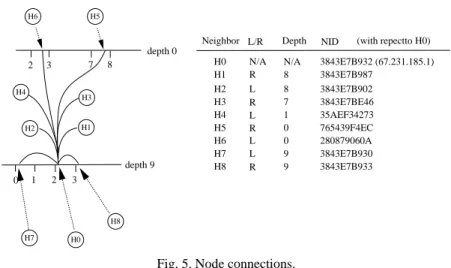
In the example in Fig. 9, there are two clusters {H1, H2, H3, H4, H5} and {H6, H7, H8,
H9, H10}, and node H2 originates a request message M. The message M is first sent to its
neighbors H1, H3, and H5. Hence, BCTL(M, H2, 1) = {H1, H2, H3, H5}. After H1 receives
M, it will not forward M to H3 because H3 is in BCTL(M, H1, 0).
H2 H6 H4 H3 H1 H5 H7 H9 H8 H10 BCTL : {H1, H3, H5, H2} Message Body BCTL : {H1, H3, H5, H2, H4} Message Body M M
Fig. 9. Broadcast in intra-cluster and inter-cluster.
H1 H2 H7 H6 H5 H3 M BCTL(M,H2,0) BCTL(M,H3,0) BCTL(M,H4,0) V.S. BCTL(M,H6,1) M H4,H3,H2,H1,H6 BCTL(M,H6,0) M H3,H2,H1,H6 M H4,H3,H2,H1 M H4,H3,H2,H1 M H4,H3,H2,H1 H4
Fig. 10. Redundant forwarding prevention on stage 1.
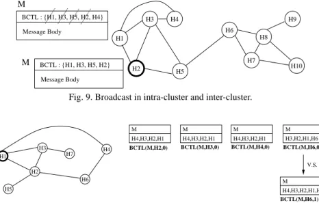
On the other hand, the capacity of BCTL affects the prevention of redundant mes-sage. In the example in Fig. 10, suppose NBLB is 4 and we setup BCTL of multiple 1. Node H1 originates a request message M to its neighbors H2, H3, and H4. With the first
H2 and H3, respectively. When M is forwarded to H6 by H2, BCTL(M, H6, 0) = {H3, H2,
H1, H6} and H4 is removed from the set because of the capacity limit of BCTL. When M
is forwarded to H4 by H6, a redundant forwarding occurs. If we setup BCTL of multiple 2,
such redundant forwarding could be prevented because BCTL(M, H6, 0) still contains
node H4.
4.2.3 Prevention for second stage
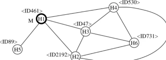
The second stage prevention focuses on the nodes by which a message is forwarded to the same destination from different sources. Before a node forwards a message, if it knows that one of its neighbors will also forward that message to the same destination, then only one node will forward it. The choice of the node by which the message is warded depends on the comparison of their NIDs. When several nodes prepare to ward the same message to the same destination, the one with the largest NID will for-ward the message. In other words, two basic requirements to fulfill the second stage pre-vention are necessary: (a) NID of each node is unique and comparable; (b) every node knows the neighbors of its neighbors.
Given a message M and a node H, NBRQ(H) is defined as the set of neighbors of node H, TS(M, H) is defined as NBRQ(H)-BCTL(M, H, 0) and NS(M, H) is defined as NBRQ(H) ∩ BCTL(M, H, 0). Notice that the notation “-” means set difference. TS(M, H) represents the remaining nodes to which M will be forwarded by H after the first stage. NS(M, H) represents the neighbors of H that are already in BCTL(M, H, 0). The concept of the second stage prevention is as follow. For each node Y in TS(M, H), if there exists a node X in NS(M, H) such that Y is a neighbor of X and the NID of X is greater than the NID of H, then H will not forward M to Y.
H1 H2 H3 H4 H6 <ID530> <ID461> <ID47> <ID2192> <ID731> H5 <ID89> M
Fig. 11. Redundant forwarding prevention on stage 2.
Consider the example in Fig. 11. The string inside the angle brackets, e.g. <ID461>, denotes the NID of the node. When message M is originated by node H1 and arrives at
nodes H2, H3, H4 and H5, the message forwardings of H2↔ H3 and H3↔ H4 are filtered
by the first stage prevention. Now consider the message forwardings H2→ H6, H3→ H6
and H4→ H6. Note that BCTL(M, H2, 0) = BCTL(M, H3, 0) = BCTL(M, H4, 0) = {H1, H2,
H3, H4, H5}. At this time, NBRQ(H3) = {H1, H2, H4, H6}, TS(M, H3) = NBRQ(H3) −
BCTL(M, H3, 0) = {H1, H2, H4, H6} − {H1, H2, H3, H4, H5} = {H6}, and NS(M, H3) = {H1,
H2, H4, H6} ∩ {H1, H2, H3, H4, H5} = {H2, H4}. Without second stage prevention, both H2
and H3 will forward M to H6. With second stage prevention, H3 discovers two facts: first,
NBRQ(H2) and NBRQ(H3) both contain the destination H6. Therefore, H3 will not
for-ward M to H6. A similar fact will also be discovered by H4. As a result, M is forwarded to
H6 only by H2. The algorithm of the SMR mechanism is given in Fig. 12.
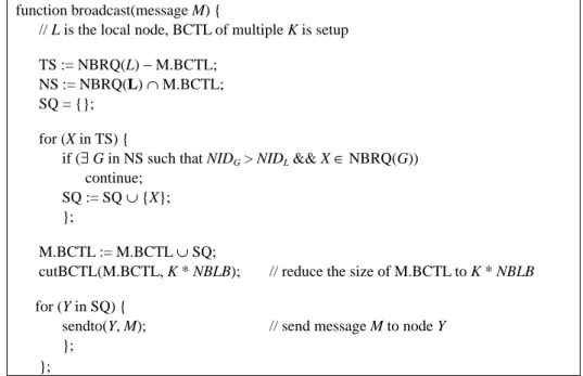
function broadcast(message M) {
// L is the local node, BCTL of multiple K is setup TS := NBRQ(L) − M.BCTL;
NS := NBRQ(L) ∩ M.BCTL; SQ = {};
for (X in TS) {
if (∃ G in NS such that NIDG > NIDL && X ∈ NBRQ(G))
continue; SQ := SQ ∪ {X}; };
M.BCTL := M.BCTL ∪ SQ;
cutBCTL(M.BCTL, K * NBLB); // reduce the size of M.BCTL to K * NBLB for (Y in SQ) {
sendto(Y, M); // send message M to node Y };
};
Fig. 12. Redundant delivery prevention in the SMR mechanism (assume BCTL of multiple 2).
The capacity of the BCTL affects the performance of the SMR mechanism. When the BCTL is full, the replacement of the BCTL adopts the first-in-first-out policy to drop the oldest nodes in BCTL. BCTL should always keeps the most recently visited nodes because the redundant message preventions at both stages concern nodes at which each message just arrived and forwarded to.
4.2.4 Clustering and topology matching
The SMR mechanism reduces redundant flooding of messages based on the cluster-ing structure of the system. The SMR mechanism works if most nodes understand where messages come from (sources) and where they are going to (destinations). Furthermore, each node should be able to identify as many of these sources and destinations as possi-ble. With a clustering structure for the system, most sources and destinations are closer. They can be identified much easier if each node knows the neighbors of their neighbors.
On the other hand, the NCC mechanism clusters the system using additional knowl-edge of Internet topology. As a consequence, nodes in the same ISP tend to form clusters. The reason to exploit topology is to achieve greater message locality, not redundant mes-sage reduction. If the NCC mechanism is modified so that Internet topology is not con-sidered (by eliminating the first two characters of each NID), the NCC mechanism still
clusters the system. And, the SMR mechanism still reduces redundant flooding of mes-sages without any loss of performance. The only drawback is lower message locality. 4.3 Experiment Verification
The SMR mechanism tries to reduce redundant messages in message floodings. We evaluate its performance by analyzing the relation between AMOR and BCTL of multi-ple K. In the following experiment, we use a BCTL of multimulti-ple 3, and NBLB is 20. The TTL (time-to-live) of each request is ∞ HOPs so that it can be flooded to every node in the system. The first part of the SMR, duplicate forwarding avoidance, is always enabled so that each message will never be forwarded indefinitely. We analyze how many redun-dant messages are reduced by the first and second stage preventions.
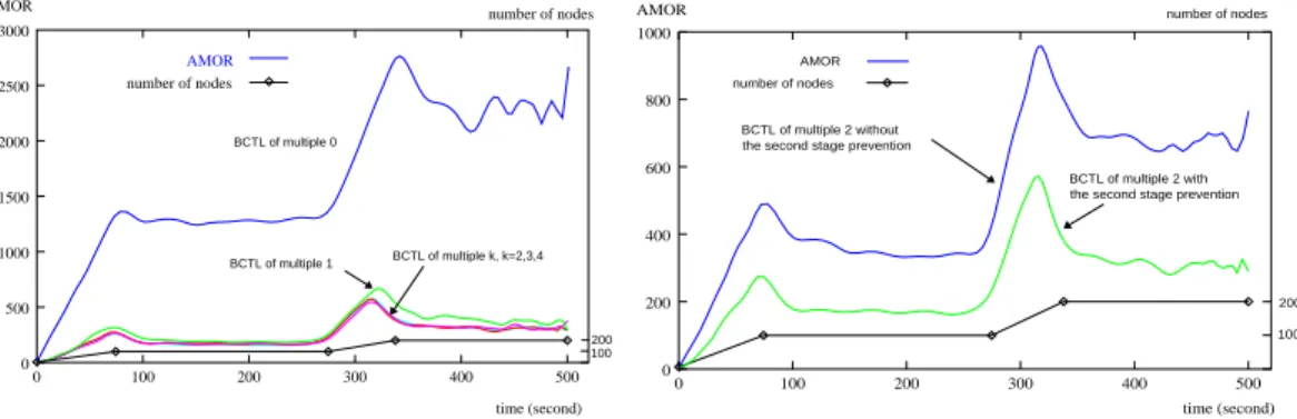
Given a system with up to 200 nodes, we first disable the second stage prevention of SMR and focus on the performance of the first stage prevention. We examine AMOR under five conditions: BCTL of multiple K, where K = 0, 1, 2, 3, and 4. The result in Fig. 13 shows that AMOR under BCTL of multiple 0 is at least six times the value under BCTL of multiple 1. AMOR under BCTL of multiple 2 can be further reduced, but the reduction slows down. AMORs under BCTL of multiple K remain almost the same value for K = 2, 3, 4. The result shows that although a larger BCTL promotes the performance of redundant forwarding prevention, it need not be very large. Ideally, the NCC mecha-nism clusters all nodes so that the number of neighbors of each node is about NBLB. Therefore, BCTL of multiple 1 should be sufficiently large to filter out most redundant messages. However, frequent joins and leaves of nodes in a real system counteract the clustering effect. A little bit larger BCTL should be better. The simulation result shows that the best choice of K is 2.
AMOR 100 200 BCTL of multiple 0 BCTL of multiple k, k=2,3,4 BCTL of multiple 1 time (second) 0 100 200 300 400 500 2500 2000 number of nodes AMOR 1500 1000 500 0 3000 number of nodes AMOR time (second) number of nodes AMOR 100 200 BCTL of multiple 2 with the second stage prevention the second stage prevention
BCTL of multiple 2 without number of nodes 0 400 300 200 100 0 1000 800 600 400 200 500
Fig. 13. Relation between AMOR and BCTL of multiple k.
Fig. 14. AMOR with and without second stage prevention.
The second part of this experiment focuses on the performance of the second stage prevention. With the first stage prevention enabled, we compare AMOR under BCTL with multiple 2 with and without the second stage prevention. Fig. 14 shows that BCTL of multiple 2 with the second stage prevention further decreases by approximately half of AMOR without the second stage prevention.
In summary, both of the first and second stage preventions indeed reduce redundant messages. Consider both Figs. 13 and 14 at a timestamp of 330. The peak of total mes-sages reaches 2750 if all preventions are disabled. However, with the first and second stage preventions enabled, the number of messages is reduced to 350. About 87.27% messages are prevented from being redundant by the SMR mechanism.
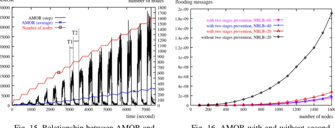
Fig. 15 shows the relation between AMOR and the number of nodes. Consider the two periods of time, T1 and T2 in Fig. 15. When the number of nodes increases from 700 to 800 in period T1, the system is not stable and AMOR increases rapidly. In period T2, the number of nodes is fixed at 800 and AMOR quickly drops to a stable lower bound. We also found that the lower bound of AMOR in the stable period is approximately O(N), where N is the number of nodes. This property illustrates that a search request generates much fewer redundant messages.
AMOR time (second) T2 T1 number of nodes 0 30000 35000 40000 45000 50000 0 1000 2000 3000 4000 5000 6000 7000 0 100 200 300 400 500 600 700 800 900 1000 1100 1200 1300 1400 1500 1600 1700 1800 20000 15000 AMOR (step) Number of nodes AMOR (average) 10000 5000 25000 number of nodes flooding messages 0 6e+08 8e+08 1e+09 1.2e+09 1.4e+09 1.6e+09 1.8e+09 2e+09 0 200 400 600 800 1000 1200 1400 1600
with two stages prevention, NBLB=60
without two stages prevention, NBLB=20
with two stages prevention, NBLB=20
with two stages prevention, NBLB=40
2e+08 4e+08
Fig. 15. Relationship between AMOR and node size.
Fig. 16. AMOR with and without second stage prevention.
Fig. 16 shows the relation between the number of flooding messages with and with-out two stages prevention for different system size N. Each node originates one request in 20 to 60 seconds, TTL of each request is ∞ HOPs, and each node maintains 40 neighbors (NBLB is 20). The result shows that although the number of flooding messages is not
O(N), the reduction in messages by two stages prevention is still very significant.
An-other factor that influences the performance of the SMR mechanism is the value of NBLB. The result also shows that NBLB of 40 can reduce more redundant flooding messages than when NBLB is 20.
On the other hand, the dynamic variation of the system also affects AMOR. The third part of our experiment initiates a system with 300 nodes. After the system is stable, it enters four dynamic variation phases. In each phase, one node leaves and one new node joins the system simultaneously every PT seconds, where PT = 4, 2, 1, and 0.5 for each phase. Fig. 17 shows that AMOR increases when PT decreases, especially when PT changes from 4 to 2 seconds and from 2 to 1 second. However, the increase becomes smaller and smaller. The result shows that the SMR mechanism adapts well to the dy-namic variation of the system.
PT=4 time (second) 100 200 300 AMOR PT=2 PT=1 PT=0.5 0 400 600 800 1000 1200 1400 1600 0 1400 1200 1000 number of nodes AMOR 800 number of nodes 600 400 200 200
Fig. 17. Relation between AMOR and dynamic variation of a system.
5. NETWORK CONNECTEDNESS
The performance of searching on a P2P system depends heavily on the connected-ness of the system. If the system is split into N components, the search hit ratio drops to 1/N in the worst case because a search request can only reach nodes of a single compo-nent. Since failures of network connections between nodes are inevitable, splitting of the system is always possible. We propose the RAL mechanism, which represents ring-around-
leader, to reconnect components if split occur.
Research [7] shows that the unstructured P2P networks are strong and robust on network connectedness, but the property is not necessarily true for our DSE system. The NCC mechanism controls connections of nodes so that the whole system is connected clusters. In Gnutella some nodes play important roles in making network connectedness strong because they maintain a large number of connections to other nodes. These con-nections also provide shortcuts for message delivery. Also, concon-nections of nodes in Gnutella seldom change. In DSE, each node maintains roughly the same number of con-nections, and moreover, connections change frequently for better system topology so that the SMR mechanism reduces redundant messages and promotes message locality. There-fore, the RAL mechanism is necessary for occasional splits of the system.
5.1 The Ring-Around-Leader Mechanism 5.1.1 Basic concept
The RAL mechanism uses message exchange among nodes to detect if a system has been split. The basic idea of RAL is simple. Each node in a connected component obtains the same unique tag. If the system is split into several disconnected components, each node in different components obtains different tags.
In the DSE system each node maintains two important pieces of information, the
NID which identify each node and one called the CID (component identification) which
is the largest NID that the node knows in the same component. The format of CID is the largest NID attached with a timestamp and the address of a special node called the leader of the component. Ideally, every node shares the same CID if the whole system is a sin-gle connected component.
The CID that each node has can be updated by message flooding or periodic mes-sage exchange between each pair of connected nodes. For the method of mesmes-sage ex-change, the CID is obtained by mutual election of nodes. When a node X joins a DSE system, the initial value of its CID, denoted CID(X), is set to its own NID, denoted
NID(X), attached with the current timestamp and its address. For each pair of connected
nodes A and B, CID(A) is compared to CID(B). If CID(A) is larger than CID(B), then B assign its CID to CID(A). Suppose that the DSE system is connected, CIDs of each node will be the largest NID of all nodes (attached with some timestamp and address) after several message exchanges. The time to generate the largest CID for every node is
O(logcN) where N is the number of nodes and C is the average number of neighbors of
each node. The node that provides the largest CID is called the leader of the component. Besides message exchange, another way to generate a global CID is by message flooding. For a given node which prepares to originate a request message, the CID of the node is put in the header of the message before it is sent out. Via the flooding of the mes-sage, the CID can be spread quickly and compared globally with CIDs of other nodes.
The CID is periodically attached with the latest timestamp by a node only when the node finds the CID (without timestamp and address) is equal to its NID. In other words, a node H is attached with its CID with current timestamp only when node H believes that it is the leader of the component. The timestamp of a CID is used to check if the CID is out of date. If a node finds the timestamp of its CID has not been updated in a long time, it is probable that either the leader (for that CID) leaves/fails or the system is split. Any node that finds its CID is out of date will treat itself as the new leader of the component, which means that it assigns its CID to be its NID attached with current timestamp and its address.
On the other hand, each node periodically checks if it is the leader. If it is it imme-diately informs all of its neighbors to build a ring connection around it (the leader). The ring assures the connectedness of the component when the leader fails or leaves the system. Leader H1 H3 H4 H5 H6 H7 H8 H9 H10 H2 H11 (ID43928,ID98290) (ID11998,ID98290) (ID47653,ID98290) (ID12048,ID98290) (ID66501,ID98290) (ID44989,ID98290) (ID85668,ID98290) (ID20009,ID98290) (ID43930,ID98290) (ID10380,ID98290) (ID98290,ID98290) Existed connections
New connections after the ring {H2, H3, H4, H6, H7} was built Fig. 18. An example for RAL: node H5 is the leader of the component.
Consider the example in Fig. 18 where each node is annotated with its (NID, CID) pair. As can be seen, all nodes form a single connected component {H1, H2, H3, H4, H5,
has the same CID and NID value, “ID98290”, which means that H5 treats itself as the
leader of the component, and hence it informs all of its neighbors to form a ring connec-tion {H2, H3, H4, H6, H7}.
5.1.2 Split recovery
Since the whole system is build based on connections between nodes, any discon-nection between nodes may split the system. Given a node which has just failed, the RAL mechanism considers two possible cases for it:
Case 1: The node is not the leader of the component.
If the failure of the node does not split the system, then the CID is still updated cor-rectly and system works as usual. Conversely, if the failure of the node does split the system, there must exist one node which first detects that the CID is out of date. The node then tries to connect to the leader of the component (by using the address attached with the CID) so that the split components can be rejoined.
In the example of Fig. 18, the failure of node H7 splits the system into two
compo-nents. No node in the component {H8, H9, H10, H11} will receive the CID with updated
timestamp from the leader H5. The CIDs of nodes H8, H9, H10 and H11 will eventually
expire. Any one of them, say H9, which first discovers that its CID expires will attempt to
contact the leader H5. Before the actual contact to H5, H9 first queries its neighbors H8,
H10 and H11 to see whether any of them has a connection to H5. If so, H9 drops the
con-nection attempt. Otherwise, H9 builds a connection to H5 so that two split components
can rejoined.
Case 2: The node is the leader of the component.
The failure of the leader of a component will never cause splitting of the component because the leader’s neighbors have formed a ring connection. This guarantees that the component remains connected even if the leader fails or leaves. In the example in Fig. 19 where the leader H5 has failed, the ring around H5, {H2, H3, H4, H6, H7}, will prevent the
component from being split. After node H5 fails or leaves, nodes in the ring around H5
will find CID “ID98290” eventually expires and replace their CIDs with their own NIDs. After several message exchanges, a new leader H3 will be elected with the new CID
“ID85668”. (ID43930,ID85668) H1 H3 H4 H6 H7 H8 H9 H10 H2 H11 (ID11998,ID85668) (ID66501,ID85668) (ID10380,ID85668) (ID47653,ID85668) (ID20009,ID85668) (ID43928,ID85668) (ID44989,ID85668) (ID12048,ID85668) (ID85668,ID85668) Leader
The RAL mechanism elects a leader of components based on message exchanges between nodes. It is possible that temporary, inconsistent leaders may exist in the system. If the system is connected, there will be only one leader after several message exchanges. If the system is split, one of these inconsistent leaders will be a bridge to connect split components. Then, there will be one leader again.
The RAL algorithm can recover the split system from single node failure. However, it can not handle massive and simultaneous failures which affect the leader and its ring. In the example of Fig. 18, if nodes {H2, H3, H4, H5, H6, H7} all fail simultaneously, the
system splits and can not be recovered by the RAL mechanism. The case of massive and simultaneous failures of nodes is not considered in the RAL mechanism.
Another related concern for the RAL mechanism is that it has to be deployed in the system from the very beginning. If some nodes, for some reason, delay to perform the RAL mechanism after they join the system, the system may risk being split and can not be recovered.
In handling the above two situations that RAL can not handle, navigators play im-portant roles. Suppose some navigators are located in different components, then a newly joined node may have a chance to rejoin some components when it connects to all navi-gators simultaneously. How to allocate navinavi-gators so that they can distribute uniformly over all nodes will be our future work on DSE.
5.1.3 Lazy update
The original RAL mechanism protects the connectedness of the system based on message exchanges of component identification between nodes. Suppose each node broadcasts its CID to its neighbors every T seconds and each node maintains NBLB + 20 neighbors. For a given system with N nodes, the total number of exchanged messages in a day is N * (NBLB + 20) * 86400/T. Such a tremendous bandwidth cost is not acceptable for a real P2P system.
We use a method called lazy-update to reduce the required bandwidth of the RAL mechanism. The lazy-update method includes two rules: (a) duplicated message ex-changes are avoided, and (b) the leader of a component spreads its CID by message flooding instead of message exchange. Rule (a) eliminates duplicated CID exchanges between nodes. Each node remembers the last CID message sent to it neighbors. Any duplicated exchange message to the same neighbor will be discarded. Rule (b) eliminates tremendous bandwidth consumption from the message exchange and speeds up CID spreading by message flooding. The flooding of CID message makes CID synchroniza-tion faster so that inconsistent CIDs will be reduced and unnecessary message exchanges can be eliminated too.
Given an N node system, we now analysis the bandwidth cost. If the system is stable and no new nodes join the system, the bandwidth cost comes only from message flooding by the leader of the component. Since each request generates at least O(N) flooding mes-sages (discussed in section 4.3), the number of flooding mesmes-sages generated in a day is at least O(N) * 86400/T assuming the leader triggers one request every T seconds.
When a new node joins the system, it takes O(logN) moves to the closest cluster (i.e., with closest neighbors). Suppose it meets NBLB + 20 new neighbors at each move
and the average number of message exchanges it handles (performed by its neighbors or itself) at each move is K, there are O(logN) * (NBLB + 20) * K exchanged messages that it sends or receives. Therefore, we can estimate the bandwidth cost of message exchange for the joining of a new node. If the new node will be the new leader of the system,
O(logN) * (NBLB + 20) * K exchanged messages are generated before it becomes a
leader. After that, it performs message flooding regularly to spread its CID.
With lazy-update, the RAL mechanism generates much fewer redundant exchange messages. Moreover, only the leader of the component and newly joined nodes trigger actions to generate messages (message flooding and message exchanges).
5.2 Experiment Verification
The RAL mechanism has the ability to reconnect a split system. We initially set up a connected system of 800 nodes. Then nodes are removed one by one. By observing the number of distinct CIDs (ignoring the attached timestamps and the addresses) with and without the RAL mechanism, we verify the performance of RAL. Notice that a system of
K components leads to K distinct CIDs.
The experiment consists of four stages. In the first stage, 800 nodes are generated and join the system one by one. In the second stage, the whole system runs into a stable status. In the meanwhile, we begin to record the number of distinct CIDs. From the be-ginning of the third stage, nodes are randomly removed from the system. At the end of the third stage, 90% of the nodes (i.e, 720 nodes) are removed. The system runs into an-other stable status from the beginning of the fourth stage.
Fig. 20 shows the number of distinct CIDs. Without the RAL mechanism, the num-ber of distinct CIDs remains high from the beginning of the second stage to the end of the fourth stage. The average number of distinct CIDs is 5.74, which means that the sys-tem is split into 5.74 components on average. With the RAL mechanism, the number of distinct CIDs remains at one from the beginning of stage 2 to the end of stage 4. The av-erage number of components is 1.48 when the RAL mechanism is enabled.
#CID=3 stage 2 stage 1 stage 3 number of nodes number of CIDs 800 80 time (second) #CID=1 stage 4 0 0 100 200 300 400 500 600 700 800 number of nodes
number of CIDs with RAIN
number of CIDs without RAIN
12 10 8 6 4 2 14
The dynamic variation of the system affects the performance of RAL. In the exam-ple of Fig. 20, there are two types of dynamic variations, the disconnections come from the NCC mechanism and failures of nodes in stage 3. These dynamic variations make the number of distinct CIDs pulsated during the period when the RAL mechanism is enabled. When the system runs into a stable status (the number of nodes is fixed and the neighbors of every node remain mostly unchanged), the pulsation of the number of distinct CIDs will stop and the number of distinct CIDs reverts gradually to one.
The last important observation is the relationship between the failure of nodes and the average number of HOPs per request. Two well-known P2P projects, Gnutella and Freenet, both suffer from the failure of nodes. Research reported in [6] shows that when the number of failed nodes exceeds a certain percentage (40% in the experiment), HO-POR grows rapidly fast in both Gnutella and Freenet. Fig. 21 shows that with the coop-eration of the NCC and RAL mechanisms, HOPOR is always below a small constant upper bound. #CID=1 stage 4 stage 2 stage 1 number of CIDs 800 80 number of nodes time (second) stage 3 0 14 0 100 200 300 400 500 600 700 800 10 number of CIDs number of nodes HOPOR 8 6 4 2 12
Fig. 21. Connectedness and HOPS in a dynamic system.
6. RELATED WORK
P2P systems can be classified as either structured systems or unstructured systems. Chord [11], CAN [6], P-Grid [8], Pastry [10], and Tapestry [9], which use DHT [4] for object placement and searching, belongs to structured P2P systems. Gnutella [15], on the other hand, search for objects by message flooding. Kazaa, another well-known P2P sys-tem [16], adopts a hierarchical structure. Powerful nodes are elected to be so called
su-pernodes which connect several clients (normal nodes) and search objects for them.
Al-though DHT based P2P systems perform excellently in searching for objects, other re-lated problems should be addressed and solved. Complex search (partial query), for ex-ample, is still difficult in a DHT network. Also, maintenance cost is another issue for any P2P system with frequent joining and cutting of nodes [17].
For unstructured P2P systems, some methods are proposed to reduce the messages originated from search requests. Research in [18] adopts a random walk to select some neighbors instead of all neighbors to send the request. Other research [19] use cache to let the search results could to be re-used by later search requests.
Research in [21] provides a cluster-based architecture which is similar to our re-search. However, neither Internet topology nor redundant message by message flooding are considered in that research. Another problem is that the method in [21] needs a cen-tral server to perform the clustering of nodes, while a cencen-tral sever causes a bottleneck for the system. Another paper [22] also adopts a cluster structure for its system, but the clustering of nodes depends on similar properties of nodes. The Internet topology and redundant message flooding are not considered.
The DSE system is an Internet topology-matching network for promoting message locality. Researches reported in [23-25] provide similar mechanisms for building topol-ogy matching systems. One major difference between them and DSE is that they use a measurement based method to evaluate the distance between nodes. Although they claim the measurement based method provides an accurate value of the distance between nodes, the method can not represent accurate communication cost between nodes. For example, a traffic jam on the route between two nodes may slow down their communication, how-ever, the communication costs between them may be very cheap. Conversely, fast com-munication may exist between two nodes which are located in different backbones. Also, the researchers try to make the system a multicast tree to reduce unnecessary traffic by cutting some connections across different AS’s (according to their distances). Such a method takes risks splitting the system and, hence, hurt the performance of the system. For our system, DSE makes the system a set of connected clusters. The SMR mechanism utilizes the benefit of clustering to reduce redundant flooding, and the RAL mechanism recovers the system if splits occur due to broken connections caused by the SMR mecha-nism or failures of nodes.
Another two related researches [26, 27] provide different methods for topology matching overlay and message routing. Research in [26] uses measured distance to some default landmark hosts to group nodes into bins. Nodes in the same bin are likely to be in the same AS. A DHT-based overlay network can be constructed on such structures to reduce message routing latency. Research [27], on the other hand, uses AS-level topology extracted from BGP reports [28] or landmark numbering (similar to [26]) to build an aux-iliary expressway network, over a normal DHT based overlay network. The expressway network is a set of powerful nodes which provide better connectivity, forwarding capac-ity, and availability. Moreover, these expressway nodes are clustered based on the above two methods to match the physical network topology. In summary, the landmark meas-urement method of [26, 27] to group nodes depends highly on availability of landmark hosts. The number of landmark hosts and how they distribute over the Internet deter-mines the precise of the method. Moreover, scalability is another problem because all nodes connect to landmark hosts for their topology-aware numbering. Our DSE system adopts HIP address format which is similar to BGP method except that DSE considers ISPID instead of ASID. The ISPID method provides three benefits. First, each ISP usu-ally provides high bandwidth pipelines between its AS’s. Second, the IP address ranges of each ISP are usually available to the public. Third, the mappings of IP addresses and ISPIDs in DSE are fulfilled by its own built-in message flooding method. No other addi-tional mechanism needs to publish the mappings.
For redundant message reduction, researches [29, 30] proposed their methods for unstructured P2P networks. Research [29] built an auxiliary tree-like sub-overlay called FloodNet within the unstructured P2P network such as Gnutella to reduce redundant
flooding messages. The research is motivated by an observation that most redundant messages are generated at their last few HOPs, but the flooding coverage expands much faster within their first few HOPs. With a tree-like overlay, each message travels by pure flooding within the low HOPs and switch to the sub-overlay for the remaining HOPs. The simulation shows that such a design reduces redundant messages but retains the same message propagation scope as that of standard floodings. One major difference between LightFlood and DSE is that the latter clusters the system topology so that most redundant messages on the same logical connections can be prevented, but the former switches the flooding of each message at the last few HOPs to FloodNet so that the mes-sage coverage expends to the same scope but with much fewer redundant mesmes-sages. No-tice that LightFlood does not change the original system topology. On the other hand, [30] proposed a peer-to-peer lookup service called Yappers over an arbitrary topology. Yap-pers groups nearby nodes to small DHTs and provides a search mechanism to traverse all the small DHTs. Such a hybrid design reduces the nodes contacted for a lookup request and, hence, reduces redundant messages. One major difference between Yappers and DSE is that Yappers focuses on key-value lookup which can be solved by DHT, while DSE concerns the reduction of redundant messages for flooding.
In comparison to well-known P2P network Kazaa, DSE provides different proper-ties. Both Kazaa and DSE adopt a hierarchical structure, but the self-organization mecha-nism of Kazaa elects so called supernodes which maintain many more connections to other normal nodes. Also, the search for files is handled by supernodes. In other words, each supernode is a small server to serve other normal nodes. The election of supernodes is based on the bandwidth and computing capacity of nodes. Powerful nodes get a higher priority to be supernodes. In DSE, every node is homogeneous. The hierarchical cluster structure is for better message routing and higher message locality. Each search request reaches every node in the DSE system to search for matched objects on local nodes. On the other hand, the election of supernodes in Kazaa requires precise measurements of the bandwidth and computing power of hosts. Frequent joins and leaves of nodes may hurt the availability of supernodes and the function they provide. These problems do not bother the DSE system because all nodes are homogeneous, and there are no nodes in DSE to become bottlenecks of the system.
The supernode structure indeed reduces traffic significantly because only super-nodes perform search requests for their clients. However, the SMR mechanism in DSE utilizes the cluster structure of nodes to reduce by up to 87.27% of the redundant traffic in message flooding.
7. CONCLUSION
The DSE system is a fully distributed and self-organizing P2P system. Our research addresses the inefficient communication in unstructured P2P systems, such as Gnutella, to propose NCC, SMR, and RAL mechanisms to improve the efficiency of communica-tion. The NCC mechanism re-constructs the topology of the system as a clustered struc-ture. The clustering of nodes depends on the logical distance between nodes. Compared to Gnutella, the NCC mechanism significantly reduces the number of messages which travel across AS’s. On the other hand, redundant message is a serious problem of the
message flooding in P2P systems. Based on the clustering structure of the system, the SMR mechanism significantly reduces redundant messages in comparison to unstruc-tured P2P systems in which forwarding of redundant flooding messages is not fully con-sidered. The last issue that we consider is the connectedness of the system. A server less P2P system organizes the whole system in a fully distributed way, hence splitting system is always possible. We proposed the RAL mechanism which handles the recovery of split components based on message exchanges between nodes. With the RAL mechanism, flooding messages can be guaranteed to reach every node in the system if necessary.
With the cooperation of the NCC, SMR and RAL mechanisms, the communication cost in P2P systems can be greatly reduced. Low-cost communication makes P2P sys-tems more scalable and perform better.
REFERENCES
1. K. Aberer, M. Punceva, M. Hauswirth, and R. Schmidt, “Improving data access in P2P systems,” IEEE Internet Computing, Vol. 6, 2002, pp. 58-67.
2. A. Oram, Peer-to-Peer Harnessing the Power of Disruptive Technologies, O’Reilly, U.S.A., 2001.
3. D. J. Watts and S. H. Strogatz, “Collective dynamics of ‘small-world’ networks,”
Nature, Vol. 393, 1998, pp. 440-442.
4. S. Ratnasamy, S. Shenker, and I. Stoica, “Routing algorithms for DHTs: some open questions,” in Proceedings of the 1st International Workshop on Peer-to-Peer
Sys-tems (IPTPS), 2002, pp. 45-52.
5. M. Ripeanu, I. Foster, and A. Iamnitchi, “Mapping the Gnutella network: properties of large-scale peer-to-peer systems and implications for system design,” IEEE
Inter-net Computing Journal, Vol. 6, 2002, pp. 50-57.
6. S. Ratnasamy, M. Handley, R. Karp, and S. Shenker, “A scalablecontent-addressable network,” in Proceedings of SIGCOMM, 2001, pp. 161-172.
7. S. Saroliu, P. Gummadi, and S. Gribble, “A measurement study of peer-to-peer file sharing systems,” in Proceedings of the Multimedia Computing and Networking (MMCN), 2002, pp. 156-170.
8. K. Aberer, “P-grid: a self-organizing access structure for P2P information systems,” in Proceedings of the 6th International Conference on Cooperative Information
Sys-tems (CoopIS), 2001, pp. 179-194.
9. B. Y. Zhao, J. Kubiatowicz, and A. D. Joseph, “Tapestry: an infrastructure for fault- tolerant wide-area location and routing,” Technical Report No. UCB/CSD-01-1141, Computer Science Division, University of California, Berkeley, 2001.
10. A. Rowstron and P. Druschel, “Pastry: scalable, decentralized object location and routing for large-scale peer-to-peer systems,” in Proceedings of the International
Conference on Distributed Systems Platforms, LNCS 2218, 2001, pp. 329-350.
11. I. Stoica, R. Morris, D. Karger, M. F. Kaashoek, and H. Balakrishnan, “Chord: a scalable peer-to-peer lookup service for internet applications,” Technical Report No. TR-819, MIT, 2001.
12. RFC 1305, Network Time Protocol, http://www.cis.ohio-state.edu/cgi-bin/rfc/rfc 1305.html.