具強韌細緻架構之可調視訊編碼演算法
151
0
0
全文
(2)
(3) 具強韌細緻架構之可調視訊編碼演算法 Scalable Video Coding Algorithms with Robust Fine Granularity Structure. 研 究 生: 黃項群 指導教授: 蔣迪豪. S t u d e n t: Hsiang-Chun Huang A d v i s o r: Dr. Tihao Chiang. 國 立 交 通 大 學 電 子 工 程 學 系 電 子 研 究 所 博 士 論 文. A Dissertation Submitted to Department of Electronics Engineering & Institute of Electronics College of Electrical and Computer Engineering National Chiao Tung University in Partial Fulfillment of the Requirements for the Degree of Doctor of Philosophy In Electronics Engineering October 2006 Hsinchu, Taiwan, Republic of China. 中 華 民 國 九十五 年 十 月.
(4)
(5) 具強韌細緻架構之可調視訊編碼演算法 學生: 黃項群. 指導教授: 蔣迪豪教授. 國立交通大學電子工程學系電子研究所 博士班. 摘要 MPEG-4 標準委員會制訂了細緻可調視訊編碼以進行視訊串流及廣 播。細緻可調視訊編碼的加強層使用了幀內預測以及位元層編碼,使 其位元流能被截斷於任意位置並提供了細緻的影像畫質調節。因為缺 乏幀間預測,MPEG-4 細緻可調視訊編碼之加強層有良好的容錯能力, 卻有較差的編碼效率。本論文提出了新的技術以加強幀間預測及編碼 效率,同時仍保有良好的錯誤容忍度。這些技術並已被正制定中的 H.264/AVC 可調視訊編碼標準所採用。 本論文首先提出了強韌細緻可調視訊編碼,利用加強層資訊以及滲 漏式預測來改善幀間預測效果。這個方法利用兩個參數,位元層數目 β (介於 0 與最大位元層數目之間)及滲漏預測係數 α(介於 0 與 1 之 間),來控制加強層參考幀的產生。α 與 β 可在不同幀之間調整,以 在加強壓縮效率及降低錯誤飄移之間取得平衡。本方法提供了整體且 彈性的架構以利更進一步的最佳化調整。加強層的資訊同時也能用來 幀間預測基礎層,以進一步加強壓縮效率。實驗結果顯示,在 MPEG-4 的測試條件下,本方法最多提供了超過 4dB 的 PSNR 改善。 本論文更進一步提出了堆疊式強韌細緻可調視訊編碼來改善強韌 細緻可調視訊編碼。堆疊式強韌細緻可調視訊編碼簡化了強韌細緻可 調視訊編碼的架構,並將其擴展為多層堆疊架構。堆疊式強韌細緻可 調視訊編碼可針對不同應用最佳化在多個操作點,並仍然保持強韌細 -i-.
(6) 緻可調視訊編碼的細緻性與容錯能力。我們同時提出一個以宏塊為基 礎,最佳化選擇 α 的方法來加強壓縮效率。我們並且提出一個單加強 層迴圈解碼結構以簡化解碼端的複雜度。實驗結果顯示,相較於強韌 細緻可調視訊編碼,堆疊式強韌細緻可調視訊編碼提供了 0.4 至 3.0dB 的 PSNR 改善。堆疊式強韌細緻可調視訊編碼已被 MPEG 委員會審閱過, 並在可調視訊編碼的 Call for Evidence 競賽中被評比為最佳技術之 一。 基於前述提出之滲漏式預測以及堆疊式架構,我們再進一步提出強 韌可調視訊編碼,以同時提供在影像大小、播放幀數、以及影像畫質 三個方面的可調視訊編碼。在影像大小以及影像畫質的可調性上,我 們提出一個只增加有限周邊資訊的彈性層間預測方式,以去除層間的 冗餘資訊。在影像畫質的可調性上,我們同時支援非細緻可調及細緻 可調視訊編碼。其中,在細緻可調視訊編碼的部分,我們擴展了 H.264/AVC 中的 CABAC 技術,使其能提供位元層編碼及細緻可調性。在 播放幀數的可調性上,我們提出一個能減少解碼端影像暫存記憶體的 實現方法。相較於 H.264/AVC 可調視訊編碼標準,強韌可調視訊編碼 提供的 PSNR 改善在-0.7dB 至+0.8dB 之間。 總結,本論文提出的強韌細緻可調視訊編碼及堆疊式強韌細緻可調 視訊編碼顯著的改善了 MPEG-4 細緻可調視訊編碼的壓縮效果,並仍保 持良好的細緻性及容錯能力。此技術也被採用於 H.264/AVC 可調視訊 編碼標準。基於前述提出之技術,我們進一步提出強韌可調視訊編碼 以同時提供在影像大小、播放幀數、以及影像畫質三個方面的可調性。 此技術並提供了能與 H.264/AVC 可調視訊編碼標準相抗衡的壓縮效 率。最後,我們還建立了一個影像串流模擬架構以展示可調視訊編碼 的應用。. - ii -.
(7) Scalable Video Coding Algorithms with Robust Fine Granularity Structure Student: Hsiang-Chun Huang. Advisor: Dr. Tihao Chiang. Department of Electronics Engineering & Institute of Electronics National Chiao Tung University. Abstract The MPEG-4 committee has defined the MPEG-4 Fine Granularity Scalability (FGS) Profile as a streaming video tool. The MPEG-4 FGS enhancement layer is intra coded with bitplane coding. It can be truncated at any location to provide fine granularity of reconstructed video quality. The lack of temporal prediction at the MPEG-4 FGS enhancement layer leads to inherent robustness at the expense of coding efficiency. In this dissertation, we propose novel techniques to improve the temporal prediction at the enhancement layer so that coding efficiency is superior to the MPEG-4 FGS. The proposed techniques are also adopted in the developing H.264/AVC SVC. We propose the Robust FGS (RFGS) that utilize enhancement layer information and leaky prediction technique to improve the temporal prediction efficiency. Our approach utilizes two parameters, the number of bitplanes β (0 ≤ β ≤ Maximal number of bitplanes) and the amount of predictive leak α (0 ≤ α ≤ 1), to control the construction of the reference frame at the enhancement layer. These parameters α and β can be selected for each frame to provide tradeoffs between coding efficiency and error drift. Our approach offers a general and flexible framework that allows further optimization. The enhancement layer is also used to predict the base layer for further improvement. Experimental results show over 4 dB PSNR improvements in coding efficiency using the MPEG-4 testing conditions. We further present Stack Robust FGS (SRFGS) to improve the RFGS performance. - iii -.
(8) SRFGS simplifies the RFGS architecture and extends it into multi-layer stack architecture. SRFGS can be optimized at several operating points to meet the requirement for various applications, while maintaining the fine granularity and error robustness of RFGS. An optimized macroblock-based alpha adaptation scheme is proposed to improve the coding efficiency. A single-loop enhancement layer decoding scheme is proposed to reduce the decoder complexity. Simulation results show that SRFGS improves the performance of RFGS by 0.4 to 3.0 dB in PSNR. SRFGS has been reviewed by the MPEG committee and ranked as one of the best algorithms in the Call for Evidence on Scalable Video Coding. Based on the proposed leaky prediction and stack structure, we further propose the Robust Scalable Video Coding (RSVC) to support spatio-temporal and SNR scalability simultaneously. To remove the inter-layer redundancy, a flexible inter-layer prediction with limited overhead is proposed for spatial and SNR scalability. For SNR scalability, both coarse granularity scalability (CGS) and FGS are supported. The H.264/AVC CABAC is extended to support the bitplane coding and FGS. A lower Decoded Picture Buffer (DPB) requirement method is used to implement the temporal scalability. The simulation results show that we have -0.7dB to +0.8dB PSNR difference comparing with the H.264/AVC SVC. In conclusion, the proposed RFGS and SRFGS architectures significantly improve the coding efficiency of MPEG-4 FGS, while still maintaining the fine granularity and error robustness. The proposed ideas have been adopted in H.264/AVC SVC. Based on leaky prediction and stack structure, we further propose RSVC to support spatio-temporal and SNR scalability simultaneously. RSVC provides comparable performance against H.264/AVC SVC. Finally, we develop a video streaming architecture for mobile WiMAX to show an application scenario of scalable video coding.. - iv -.
(9) Acknowledgement 能完成論文,首先要感謝蔣迪豪老師的指導。蔣老師提供了有趣又有挑戰性的研 究題目,讓我在研究討論的過程中逐步學習成長。蔣老師也提供了國際性的研究 計畫及競賽,在研究及競爭的過程中,讓我學到難得的經驗,並增加了國際視野。 而在學校的研究之外,蔣老師在工作的選擇上也給我許多建議。另外,我也非常 謝謝蔣老師這幾年來在各方面給我的幫助及鼓勵。 再來,我要感謝杭學鳴老師。杭老師除了在研究討論時給我很多的指導外,杭老 師待人處事的態度,也是我最需要學習的。另外,我也要感謝俊能及文孝兩位學 長。兩位學長多年來在研究,論文寫作,以及上台報告各方面,都給我非常多的 建議及指導。此外,我也要感謝俊毅,士豪,志鴻,家揚,耀中,以及其他 Commlab 的同學們,在各方面給我的幫助。我也要謝謝 Ambarella 的上司及同事們,在過 去幾年裡,不時的幫忙減少或分擔我的工作,讓我有時間繼續學校的研究。 最後,我要謝謝我的母親多年來對我的支持,照顧及教育,讓我能自由自在,無 後顧之憂的選擇自己的人生,做自己想做的事。我還要感謝老天爺,總是給我足 夠的幸運。. -v-.
(10) To my mother. - vi -.
(11) Contents. 摘要 ............................................................................................................................................................. I ABSTRACT............................................................................................................................................. III ACKNOWLEDGEMENT........................................................................................................................ V CONTENTS ........................................................................................................................................... VII LIST OF FIGURES .................................................................................................................................. X LIST OF TABLES.................................................................................................................................. XII LIST OF NOTATIONS........................................................................................................................ XIII CHAPTER 1 INTRODUCTION ..............................................................................................................1 1.1 OVERVIEW OF DISSERTATION .....................................................................................................1 1.1.1 Scalable Video Coding Standard ...............................................................................................4 1.1.2 Robust Fine Granularity Scalability (RFGS).............................................................................4 1.1.3 Stack Robust Fine Granularity Scalability (SRFGS).................................................................5 1.1.4 Relevance to H.264/AVC SVC..................................................................................................6 1.1.5 Robust Scalable Video Coding (RSVC) ....................................................................................6 1.1.6 Streaming Video Application.....................................................................................................6 1.2 ORGANIZATION AND CONTRIBUTION .........................................................................................7 CHAPTER 2 SCALABLE VIDEO CODING STANDARD.................................................................10 2.1 MPEG-4 FGS..........................................................................................................................10 2.2 H.264/AVC SVC ..................................................................................................................... 11 2.2.1 Overview ................................................................................................................................. 11 2.2.2 Overall Encoder Structure .......................................................................................................12 2.2.3 Temporal Scalability................................................................................................................15 2.2.3.1 Motion Compensated Temporal Filtering......................................................................................... 15 2.2.3.2 Hierarchical-B Structure .................................................................................................................. 16 2.2.3.3 Adaptive Reference Fine Granularity Scalability ............................................................................. 17. 2.2.4 SNR Scalability .......................................................................................................................19 2.2.4.1 Coarse Grain Scalability (CGS) ....................................................................................................... 19 2.2.4.2 Fine Grain Scalability (FGS)............................................................................................................ 19. 2.2.5 Spatial Scalability....................................................................................................................20 2.2.5.1 Inter-layer Prediction Structure ........................................................................................................ 21 2.2.5.2 Intra Texture Prediction.................................................................................................................... 22 2.2.5.3 Motion Prediction ............................................................................................................................ 23 2.2.5.4 Residue prediction............................................................................................................................ 23. 2.2.6 Interlaced Coding ....................................................................................................................24 2.2.7 Bit stream Extraction and Adaptation......................................................................................25 2.2.7.1 Simple Truncation ............................................................................................................................ 25 2.2.7.2 Quality Layer Adaptation ................................................................................................................. 25. 2.2.8 Performance Comparison between H.264/AVC and H.264/AVC SVC ...................................26 2.2.8.1 H.264/AVC SVC with Spatial Scalability Only ............................................................................... 26 2.2.8.2 H.264/AVC SVC with SNR Scalability Only................................................................................... 27 2.2.8.3 H.264/AVC SVC with Combined Scalability................................................................................... 27. 2.2.9 Summary .................................................................................................................................29. - vii -.
(12) CHAPTER 3 ROBUST FINE GRANULARITY SCALABILITY (RFGS) ........................................30 3.1 INTRODUCTION ........................................................................................................................30 3.2 PREDICTION TECHNIQUES OF THE ENHANCEMENT LAYER .......................................................31 3.2.1 Leaky Prediction......................................................................................................................32 3.2.2 Partial Prediction .....................................................................................................................32 3.2.3 Adaptive Mode Selection.........................................................................................................34 3.3 THE RFGS SYSTEM ARCHITECTURE ........................................................................................35 3.3.1 Functional Description ............................................................................................................40 3.3.2 Leaky and Partial Prediction....................................................................................................40 3.3.3 Analysis of Error Propagation .................................................................................................42 3.3.4 High Quality Reference in Base Layer ....................................................................................46 3.3.5 Rate Control for the Enhancement Layer ................................................................................48 3.4 THE SELECTION OF THE RFGS PARAMETERS ...........................................................................49 3.4.1 Selection of the Leaky Factor..................................................................................................49 3.4.2 The Number of Bitplanes ........................................................................................................53 3.5 EXPERIMENT RESULT AND ANALYSES ......................................................................................54 3.5.1 The Testing Conditions............................................................................................................54 3.5.2 Performance Comparisons.......................................................................................................56 3.5.3 Test for Error Recovery Capability..........................................................................................58 3.6 SUMMARY ................................................................................................................................61 CHAPTER 4 STACK ROBUST FINE GRANULARITY SCALABILITY (SRFGS) .......................63 4.1 INTRODUCTION ........................................................................................................................63 4.2 SIMPLIFIED RFGS PREDICTION SCHEME .................................................................................64 4.3 ENHANCED PREDICTION ARCHITECTURE USING STACK CONCEPT...........................................69 4.4 THE STACK RFGS SYSTEM ARCHITECTURE ............................................................................72 4.4.1 Functional Description ............................................................................................................72 4.4.2 Optimized macroblock-based alpha adaptation .......................................................................77 4.4.3 Prediction scheme of B-frame .................................................................................................77 4.4.4 Stack RFGS with single-loop enhancement layer decoder......................................................78 4.5 EXPERIMENT RESULTS AND ANALYSES ....................................................................................81 4.6 SUMMARY ................................................................................................................................85 CHAPTER 5 RELEVANCE TO THE H.264/AVC SVC.......................................................................86 5.1 5.2 5.3 5.4. INTRODUCTION ........................................................................................................................86 RFGS IN H.264/AVC SVC ......................................................................................................86 SRFGS IN H.264/AVC SVC....................................................................................................88 SUMMARY ................................................................................................................................91. CHAPTER 6 ROBUST SCALABLE VIDEO CODING ......................................................................92 6.1 INTRODUCTION ........................................................................................................................92 6.2 THE RSVC SYSTEM ARCHITECTURE .......................................................................................93 6.3 SPATIAL SCALABILITY AND SNR SCALABILITY ........................................................................95 6.3.1 Texture Prediction....................................................................................................................95 6.3.2 Prediction-Information Prediction ...........................................................................................96 6.3.3 Residue Prediction...................................................................................................................97 6.3.4 Skip Mode ...............................................................................................................................97 6.4 FINE GRANULARITY SCALABILITY (FGS) ................................................................................98 6.4.1 Entropy Coding .......................................................................................................................98 6.4.2 Leaky Prediction.................................................................................................................... 102 6.5 TEMPORAL SCALABILITY ....................................................................................................... 102 6.6 BITSTREAM EXTRACTION AND ERROR CONCEALMENT.......................................................... 104 6.6.1 Bitstream Extraction.............................................................................................................. 104 6.6.2 Error Concealment................................................................................................................. 105 6.7 SIMULATION RESULTS ............................................................................................................ 105 6.7.1 Spatial Scalability.................................................................................................................. 108 6.7.2 SNR Scalability ..................................................................................................................... 108 6.7.3 Combined Scalability ............................................................................................................ 110 6.8 SUMMARY .............................................................................................................................. 112 - viii -.
(13) CHAPTER 7 CONCLUSION ............................................................................................................... 113 APPENDIX A STREAMING VIDEO APPLICATION BASED ON H.264/AVC SVC FOR MOBILE WIMAX ................................................................................................................................. 116 A.1 INTRODUCTION ...................................................................................................................... 116 A.2 SYSTEM ARCHITECTURE ........................................................................................................ 117 A.1.1 Overview of the System Architecture................................................................................... 117 A.1.2 The H.264/AVC SVC Streaming Server............................................................................... 118 A.1.3 The Mobile WiMAX Simulation Platform ........................................................................... 120 A.3 SIMULATION RESULTS ............................................................................................................ 121 A.1.4 Test Conditions ..................................................................................................................... 121 A.1.5 Simulation results ................................................................................................................. 123 A.4 SUMMARY .............................................................................................................................. 126 BIBLIOGRAPHY .................................................................................................................................. 128 CURRICULUM VITAE ........................................................................................................................ 131. - ix -.
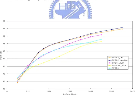
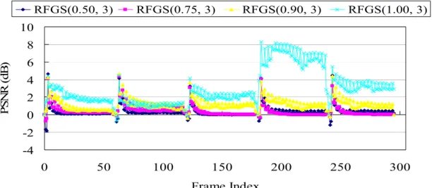
(14) List of Figures. FIGURE 1.1. AN EXAMPLE OF SVC (A) APPLICATION SCENARIO (B) BIT STREAM EXTRACTION, AND (C) THE DECODED VIDEO ..................................................................................................................................3 FIGURE 2.1. MPEG-4 FGS ENCODER STRUCTURE ...................................................................................... 11 FIGURE 2.2. H.264/AVC SVC ENCODER STRUCTURE WITH THREE SPATIAL/SNR LAYERS ...........................13 FIGURE 2.3. TEMPORAL DECOMPOSITION ....................................................................................................14 FIGURE 2.4. CONFIGURATION OF INTER-LAYER PREDICTION .......................................................................21 FIGURE 2.5. PERFORMANCE COMPARISON BETWEEN H.264/AVC AND H.264/AVC SVC............................28 FIGURE 3.1. PARTIAL INTER PREDICTION MODE FOR CODING THE BITPLANES AT THE ENHANCEMENT LAYER USING RFGS CODING FRAMEWORK. EACH FRAME HAS THE FLEXIBILITY TO SELECT THE NUMBER OF BITPLANES USED TO GENERATE THE HIGH QUALITY REFERENCE FRAME. FOR EXAMPLE, THE FIRST FRAME USES THREE BITPLANES TO COMPUTE THE HIGH QUALITY REFERENCE FRAME. ......................33 FIGURE 3.2. CHANNEL BANDWIDTH VARIATION PATTERN FOR THE DYNAMIC TEST DEFINED IN THE MPEG DOCUMENT M8002 [19]. ....................................................................................................................35 FIGURE 3.3. DIAGRAM OF THE RFGS ENCODER FRAMEWORK. THE SHADOWED BLOCKS ARE THE NEW MODULES FOR RFGS AS COMPARED TO MPEG-4 BASELINE FGS......................................................37 FIGURE 3.4. DIAGRAM OF THE RFGS DECODER FRAMEWORK. THE SHADOWED BLOCKS ARE THE NEW MODULES FOR RFGS AS COMPARED TO MPEG-4 BASELINE FGS......................................................38 FIGURE 3.5. ILLUSTRATION OF A TRANSMISSION SCENARIO WITH CORRUPTED OR LOST FRAME FOR A VIDEO STREAM OF N FRAMES, WHERE THE ENHANCEMENT LAYER OF THE I-TH FRAME IS ASSUMED TO BE LOST. .................................................................................................................................................45 FIGURE 3.6 THE VISUAL QUALITIES OF THE RECONSTRUCTED PICTURES USING THE PROPOSED RFGS RATE CONTROL SCHEME. WE PROVIDE THE QUALITY OF THE FIRST 60 FRAMES OF THE FOREMAN BITSTREAM. THE BASE LAYER BITSTREAM IS ENCODED WITH A BITRATE OF 256KBPS. THE ENHANCEMENT LAYER BITSTREAM IS TRUNCATED AT SEVERAL BITRATES TO UNDERSTAND THE VARIATION IN PSNR FOR VARIOUS CHANNEL BANDWIDTHS. THE RESULTS SHOW THAT THE PSNR VARIATION IS SMALLER THAN 2 DB AT VARIOUS BITRATE. ..................................................................48 FIGURE 3.7. THE LINEAR DEPENDENCY BETWEEN NEAR-OPTIMAL LEAK FACTOR AND THE PICTURE QUALITY IN PSNR OF THE BASE LAYER. THE FRAMES WITHIN FIVE GOVS, WHERE EACH HAS 60 FRAMES, ARE USED FOR THE SIMULATIONS WITH THE FOUR SEQUENCES, NAMELY AKIYO, CARPHONE, FOREMAN, AND COASTGUARD. ...........................................................................................................................50 FIGURE 3.8. PSNR VERSUS BITRATE COMPARISON BETWEEN FGS, RFGS AND SINGLE LAYER CODING SCHEMES FOR THE Y COMPONENT OF THE FOREMAN SEQUENCE, WHERE. β. IS 3. WE USE THREE. DIFFERENT CODING SCHEMES INCLUDING ‘RFGS1’, ‘RFGS2_NEAROPT’, AND ‘RFGS2_LM’ IN THE EXPERIMENTS. ‘RFGS1’ USE THE RFGS ALGORITHM FOR THE ENHANCEMENT LAYER ONLY. ‘RFGS2’ USES THE RFGS ALGORITHM FOR BOTH THE ENHANCEMENT AND BASE LAYERS. ‘NEAROPT’ MEANS THE RESULT OF THE NEAR-OPTIMAL APPROACH AND ‘LM’ MEANS THE RESULTS USING THE PROPOSED LINEAR MODEL. .................................................................................................................................51 FIGURE 3.9 PSNR VERSUS BITRATE COMPARISON BETWEEN FGS, RFGS AND SINGLE LAYER CODING SCHEMES FOR THE Y COMPONENT OF THE COASTGUARD SEQUENCE, WHERE. β. IS 3. WE USE THREE. DIFFERENT CODING SCHEMES INCLUDING ‘RFGS1’, ‘RFGS2_NEAROPT’, AND ‘RFGS2_LM’ IN THE EXPERIMENTS. ‘RFGS1’ USE THE RFGS ALGORITHM FOR THE ENHANCEMENT LAYER ONLY. ‘RFGS2’ USES THE RFGS ALGORITHM FOR BOTH THE ENHANCEMENT AND BASE LAYERS. ‘NEAROPT’ MEANS THE RESULT OF THE NEAR-OPTIMAL APPROACH AND ‘LM’ MEANS THE RESULTS USING THE PROPOSED LINEAR MODEL. .................................................................................................................................52 FIGURE 3.10. PSNR VERSUS BITRATE COMPARISON BETWEEN FGS, RFGS AND SINGLE LAYER CODING. -x-.
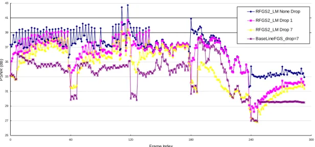
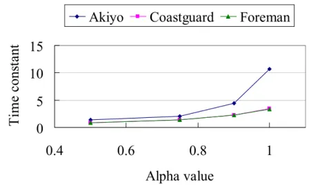
(15) SCHEMES FOR THE Y COMPONENT OF THE AKIYO SEQUENCE, WHERE. β. IS 3. WE USE THREE. DIFFERENT CODING SCHEMES INCLUDING ‘RFGS1’, ‘RFGS2_NEAROPT’, AND ‘RFGS2_LM’ IN THE EXPERIMENTS. ‘RFGS1’ USES THE RFGS ALGORITHM FOR THE ENHANCEMENT LAYER ONLY. ‘RFGS2’ USES THE RFGS ALGORITHM FOR BOTH THE ENHANCEMENT AND THE BASE LAYERS. ‘NEAROPT’ MEANS THE RESULT OF THE NEAR-OPTIMAL APPROACH AND ‘LM’ MEANS THE RESULTS USING THE PROPOSED LINEAR MODEL. ................................................................................................................52. FIGURE 3.11. PSNR VERSUS BITRATE COMPARISON BETWEEN VARIOUS VALUES OF RFSG PARAMETER β FOR THE Y COMPONENT OF THE FOREMAN SEQUENCE, WHERE THE LEAK FACTOR α IS SELECTED WITH THE PROPOSED LINEAR MODEL. .........................................................................................................53 FIGURE 3.12 PSNR VERSUS BITRATE COMPARISON BETWEEN RFGS AND PFGS FOR THE Y COMPONENT OF THE COASTGUARD AND FOREMAN SEQUENCES IN CIF FORMAT USING THE TEST CONDITION A IN THE MPEG DOCUMENT M6779 [18]. FOR RFGS, β IS 3............................................................................55 FIGURE 3.13 PSNR VERSUS BITRATE COMPARISON BETWEEN RFGS AND PFGS FOR THE Y COMPONENT OF THE COASTGUARD AND FOREMAN SEQUENCES IN CIF FORMAT USING THE TEST CONDITION B FROM THE MPEG DOCUMENT M6779 [18]. FOR THE RFGS, β IS 3..............................................................56 FIGURE 3.14. SAMPLE BANDWIDTH PROFILE TO TEST THE ERROR RECOVERY CAPABILITY OF THE RFGS TECHNIQUE........................................................................................................................................58 FIGURE 3.15. THE ERROR ATTENUATION IN PSNR FOR THE Y COMPONENT OF THE AKIYO SEQUENCE UNDER DIFFERENT α IN THE RFGS1 FRAMEWORK, WHERE THE PAIR OF THE VALUES INDICATES THE PREDICTION MODE PARAMETERS (α , β ) . ..........................................................................................59 FIGURE 3.16. THE ERROR ATTENUATION IN PSNR FOR THE Y COMPONENT OF THE FOREMAN SEQUENCE USING THE RFGS2_LM FRAMEWORK. ALL THE CURVES DENOTE TRUNCATION OF THE ENHANCEMENT LAYER BITSTREAM AT 1024KBPS. FOR THE CURVE LABELED ‘RFGS2_LM DROP 1’, THE FIRST FRAME OF EACH GOV IS DROPPED. FOR THE CURVE LABELED ‘RFGS2_LM DROP 7’, THE FIRST SEVEN FRAMES OF EACH GOV ARE DROPPED. FOR THE CURVE LABELED ‘RFGS2_LM NONE DROP’, NO FRAME IS DROPPED. THE CURVE LABELED ‘BASELINEFGS_DROP=7’ IS THE BASELINE FGS WITH THE FIRST 7 FRAMES OF EACH GOV DROPPED. .........................................................................................60 FIGURE 3.17. THE RELATIONSHIP BETWEEN THE LEAK FACTOR α AND THE TIME CONSTANT τ FOR THE ERROR ATTENUATION. FOR EACH CURVE, β IS 3...............................................................................61 FIGURE 3.18. THE COMPARISON OF VISUAL QUALITY IN PSNR BETWEEN FGS AND SINGLE LAYER APPROACHES WITH THE DYNAMIC TEST CONDITION AS DEFINED IN THE MPEG DOCUMENT M8002 [19]. ..................................................................................................................................................62 FIGURE 4.1 THE ORIGINAL RFGS ENCODER ................................................................................................66 FIGURE 4.2 THE SIMPLIFIED RFGS ENCODER .............................................................................................68 FIGURE 4.3 SRFGS PREDICTION CONCEPT ...............................................................................................71 FIGURE 4.4 DIAGRAM OF THE SRFGS ENCODER FRAMEWORK ...................................................................73 FIGURE 4.5 DIAGRAM OF THE SRFGS DECODER FRAMEWORK ...................................................................75 FIGURE 4.6 THE SRFGS ENHANCEMENT LAYER BITSTREAM FORMAT .........................................................76 FIGURE 4.7 DIAGRAM OF THE SRFGS SINGLE-LOOP ENHANCEMENT LAYER DECODER FRAMEWORK ..........80 FIGURE 4.8 PSNR VERSUS BITRATE COMPARISON BETWEEN SRFGS, RFGS AND AVC CODING SCHEMES FOR THE Y COMPONENT. ....................................................................................................................83 FIGURE 6.1. RSVC ENCODER STRUCTURE WITH THREE SPATIAL/SNR LAYERS............................................94 FIGURE 6.2. PROBABILITY DISTRIBUTION OF THE RESIDUE VALUE CAN BE APPROXIMATE BY A LAPLACIAN MODEL, WHERE SMALLER VALUE HAS LARGER PROBABILITY........................................................... 100 FIGURE 6.3. HIERARCHICAL PREDICTION STRUCTURE IMPLEMENTATION .................................................. 103 FIGURE 6.4. SIMULATION RESULTS FOR SPATIAL SCALABILITY................................................................... 107 FIGURE 6.5. SIMULATION RESULTS FOR CGS AND FGS ENTROPY IN RSVC. ............................................. 109 FIGURE 6.6. SIMULATION RESULTS FOR SNR SCALABILITY WITH FGS...................................................... 110 FIGURE 6.7. SIMULATION RESULTS FOR COMBINED SCALABILITY. ............................................................. 111 FIGURE A.1 SVC VIDEO STREAMING ARCHITECTURE ................................................................................ 118 FIGURE A.2 THE TRANSMITTED GOPS IN EACH REPORT PERIOD. .............................................................. 119 FIGURE A.3 THE SDU FAILURE RATE IN 1-CONNECTION SERVICE.............................................................. 123 FIGURE A.4 THE DATA RATE IN 1-CONNECTION SERVICE. .......................................................................... 123 FIGURE A.5 THE SDU FAILURE RATE IN 2-CONNECTION SERVICE.............................................................. 125 FIGURE A.6 THE DATA RATE IN 2-CONNECTION SERVICE. .......................................................................... 125 FIGURE A.7 THE PSNR RESULTS OF THE STREAMING SERVICES. ............................................................... 126. - xi -.
(16) List of Tables. TABLE 3.1. TERMINOLOGY OF THE RFGS CODING FRAMEWORK.................................................................39 TABLE 4.1 THE VALUE OF (Α, Β) USED IN THE SIMULATION..........................................................................82 TABLE A.1 THE AVERAGE BITRATE OF THE SVC BITSTREAM AT VARIOUS SPATIAL-SNR AND TEMPORAL RESOLUTIONS .................................................................................................................................. 121. - xii -.
(17) List of Notations (⋅)mc. Operation of motion compensation. α. The leaky factor that multiply on the enhancement layer information. β. The number of enhancement layer bitplane used for inter prediction. i. The time index of the image.. BLPI. Predicted base layer frame that is generated by motion compensation from the base layer frame buffer.. ELPI. Predicted frame of the enhancement layer that is generated by motion compensation from the enhancement layer frame buffer.. MCFDBL. Motion compensated frame difference of the base layer, which is the difference between BLPI and the original image.. MCFDEL. Motion compensated frame difference of the enhancement layer which the difference between ELPI and the original image.. HQRI. High quality reference image, which is stored in the enhancement layer frame buffer to generate the high quality prediction image ELPI.. ELRI. Enhancement layer reconstructed image, which is the summation of ELPI, Bˆ , and Dˆ . ELRI will be processed by the leaky factor to generate the HQRI.. F. The original image before encoding.. B. The base layer reconstructed image, which is the summation of BLPI and Bˆ . B will be stored in the base layer frame buffer.. D. The final residual used at the enhancement layer prediction loop - xiii -.
(18) in the encoder. (B+αD) will be stored at the enhancement layer frame buffer of the encoder.. Bˆ. Coded DCT coefficients of frame MCFDBL. The Bˆ before de-quantization will be compressed as the base layer bitstream.. Dˆ. Difference signal between MCFDEL and Bˆ for P-pictures or MCFDBL and Bˆ for I-pictures and B-pictures. Dˆ will be compressed as the enhancement layer bitstream.. ( D. The received Dˆ in the decoder side. Since there may be truncation or error during the transmission of enhancement ( layer bitstream, Dˆ and D may be different.. ΔDˆ. ( The difference between Dˆ and D .. ~ D. ~ The reconstructed D in the decoder side. ( B + αD ) will be stored at the enhancement layer frame buffer of the decoder.. QE. Quantization error.. - xiv -.
(19) CHAPTER 1 Introduction. Introduction. 1.1. Overview of Dissertation. The delivery of multimedia information to mobile device over wireless channels and/or Internet is a challenging problem because multimedia transportation suffers from bandwidth fluctuation, random errors, burst errors and packet losses [10]. Thus, the MPEG-4 committee has adopted various techniques to address the issue of error-resilient delivery of video information for multimedia communications. However, it is even more challenging to simultaneously stream or multicast video over Internet or wireless channels to a wide variety of devices where it is impossible to optimize video quality for a particular device, bitrate and channel conditions. The compressed video information is lost due to congestion, channel errors and transport jitters. The temporal predictive nature of most compression technology causes the undesirable effect of error propagation. To address the broadcast or Internet multicast applications, the ideas of Scalable Video Coding (SVC) is proposed. The SVC provides a single bitstream that can be easily adapted to support various bandwidths and clients. It can be used for various applications such as multi-resolution content analysis, content adaptation, complexity adaptation and bandwidth adaptation. For example, when the video is transported over error-prone channels with fluctuated bandwidth for Internet or wireless visual. -1-.
(20) communications, the clients, consisting of various devices, requires different processing power and spatio-temporal resolutions. To serve diversified clients over heterogeneous networks, the SVC allows on-the-fly adaptation in the spatio-temporal and quality dimensions according to the network conditions and receiver capabilities. During transmission, the server or router truncates the bit stream to match the available bandwidth. Moreover, the client can skip parts of the received bit stream to match its capability in execution cycles and display dimension. Figure 1.1 illustrates an application scenario for SVC. In Figure 1.1 (a), the system contains 3 devices including server, router, and wireless access point with different connection speeds. Multiple clients are connected to the networks. The SVC bit stream has 1) 2 spatial resolutions: Standard Definition (SD, 704x576) and Common Intermediate Format (CIF, 352x288); 2) 3 temporal resolutions: 60 frames per second (fps), 30 fps, and 15 fps; and 3) 3 Signal-to-Noise-Ratio (SNR) layers for each spatial resolution. Figure 1.1 (b) shows the bit stream structure for each connection. The bit stream consists of multiple pictures and each picture contains several spatial and quality resolutions. Initially, the video server retains only the first three SNR layers at the CIF resolution and the first and part of the second SNR layers at the SD resolution to match the 4 Mbps bandwidth between the video server and the router. To match the 3Mbps bandwidth between the router and the wireless access point, the router discards the bit stream for the second SNR layer at the SD resolution and the additional temporal resolutions for 60 fps. Similarly, the two wireless clients of lower complexity and display resolution are supported with further truncation. The spatio-temporal pyramid is illustrated in Figure 1.1 (c).. -2-.
(21) 3Mbps. SVC Video Server (SD@3SNR,60fps) (Full resolution) (6Mbps) 0. 4. 2. 1. 3. 0. 4. 8. 0 4 2 80 8 6. 0Kbp s. s Kbp 200. s bp 4M 1 3. 0 4 2 8. Router. Wireless AP. 2. ([email protected],30fps). 048. 8. ([email protected],60fps). (SD@1SNR,30fps). (CIF@1SNR,15fps). (a) SVC application scenario (SD@3SNR,60fps) (Full resolution). Pic0. ([email protected],60fps). Pic0. (SD@1SNR,30fps). Pic0. ([email protected],30fps) Pic0. Pic4. Pic4. Pic4. Pic4 Pic2. Pic2. Pic2. Pic8. Pic2. Pic8. Pic1. Pic1. Pic3. Pic3. Pic8. Pic8. Pic6. Pic5. Pic6 Spatial/SNR layers In each picture Cif Cif Cif SD SD snr0 snr1 snr2 snr0 snr1. Pic6. SD snr2. (CIF@1SNR,15fps) 0 4 8. (b) SVC bit stream extraction (SD@3SNR,60fps) (Full resolution). SD snr2. ([email protected],60fps). SD snr1. (SD@1SNR,30fps). SD snr0 ([email protected],30fps). Cif snr2 Cif snr1. (CIF@1SNR,15fps). Cif snr0 Pic0. Pic1. Pic2. Pic3. Pic4. Pic5. Pic6. Pic7. Pic8. (c) SVC decoded video Figure 1.1. An example of SVC (a) application scenario (b) bit stream extraction, and (c) the decoded video. -3-.
(22) 1.1.1 Scalable Video Coding Standard There are two scalable video coding standards developed in these years. The ISO/IEC MPEG-4 committee defined the Fine Granularity Scalability (FGS) that provides a DCT-based scalable approach in a layered fashion. The base layer is coded by a non-scalable MPEG-4 advanced simple profile (ASP) while the enhancement layer is intra coded with embedded bit plane coding to achieve fine granular scalability. The lack of temporal prediction at the FGS enhancement layer leads to inherent robustness at the expense of coding efficiency. To further improve the coding efficiency of SVC, recently the ISO/IEC MPEG and ITU-T VCEG form the Joint Video Team (JVT) to develop the scalable video coding amendment of the H.264/AVC standard [1][2][3] (refer to as “H.264/AVC SVC” in this dissertation). The H.264/AVC SVC technology consists of hierarchical-B structure with leaky prediction. To enhance coding efficiency among coding layers, it adopts adaptive inter-layer prediction techniques including intra texture, motion, and residue predictions. The constrained inter-layer prediction is used for reduced decoder complexity. A cyclic block coding is used for SNR scalability with better subjective quality.. 1.1.2 Robust Fine Granularity Scalability (RFGS) The lack of temporal prediction at the MPEG-4 FGS enhancement layer leads to inherent robustness at the expense of coding efficiency. Our goal is constructing a prediction structure that utilizes the enhancement layer information to improve the prediction efficiency, while still maintaining the robustness when the enhancement layer bitstream is truncated. We proposed the Robust FGS (RFGS) that utilize the leaky prediction concept to improve the temporal prediction efficiency while keeping the features of fine granularity and robustness of MPEG-4 FGS. RFGS multiplies the enhancement layer -4-.
(23) temporal prediction information by a leaky factor α, where 0 ≤ α ≤ 1. With utilizing the enhancement layer information, the prediction efficiency improved significantly. When error occurs in the enhancement layer, it is multiplied with the leaky factor α every time when forming the temporal prediction frames. After several iterations, the error is attenuated to zero and no longer drift. RFGS further provides another factor β to control the number of bit planes used in the enhancement layer prediction loop. These parameters α and β can be selected for each frame to provide tradeoffs between coding efficiency and error drift. To further improve the coding efficiency, RFGS can also use the enhancement layer information to predict the base layer. Our experimental results show over 4 dB improvements in coding efficiency using the MPEG-4 testing conditions.. 1.1.3 Stack Robust Fine Granularity Scalability (SRFGS) In the RFGS approach, Larger β leads to more enhancement layer information used for temporal prediction. With the removal of more temporal redundancy, larger β provides better performance when all the reference bit planes are fully reconstructed. However, larger β may lead to larger drifting error at lower bitrate as less amount of required reference information is available for motion compensation. On the contrary, smaller β reduce the drift at lower bitrate at the expense of coding efficiency because the bit planes after β effectively become intra-coded with less coding performance. We propose the Stack RFGS (SRFGS) to solve the problem. In SRFGS, the RFGS architecture is extended to multi-layer stack architecture. Each layer has its own prediction loops. The error in a layer will not affect the data in other layers. This error localization feature reduces the drifting error because when the higher enhancement layer information is truncated, the lower enhancement layer still can be decoded -5-.
(24) correctly. The simulation results show that SRFGS can improve the performance of RFGS by 0.4 to 3.0 dB in PSNR.. 1.1.4 Relevance to H.264/AVC SVC Although the RFGS and SRFGS framework were originally developed based on the MPEG-4 FGS structure, the same prediction structure can also be applied for H.264/AVC SVC. In H.264/AVC SVC, the RFGS prediction structure is adopted and extended to adapt the leaky factor at the coefficient level. The SRFGS prediction structure is adopted and modified to reduce the decoder complexity. The simulation results show that the RFGS and SRFGS prediction structure have up to 4dB and 2dB PSNR improvement in the H.264/AVC SVC, respectively.. 1.1.5 Robust Scalable Video Coding (RSVC) Based on the proposed leaky prediction and stack structure, we further propose the Robust Scalable Video Coding (RSVC) to support spatio-temporal and SNR scalability simultaneously. To remove the inter-layer redundancy, a flexible inter-layer prediction with limited overhead is proposed to for the spatial and SNR scalability. For SNR scalability, both coarse granularity scalability (CGS) and FGS are supported. The H.264/AVC CABAC is extended to support the bitplane coding and FGS. A lower Decoded Picture Buffer (DPB) requirement method is used to implement the temporal scalability. The simulation results show we have -0.7dB to +0.8dB PSNR difference comparing with the developing H.264/AVC SVC.. 1.1.6 Streaming Video Application To demonstrate the application scenario of SVC, we further establish a video streaming architecture based on H.264/AVC SVC for mobile WiMAX. The performance of SVC and non-SVC using both single and multiple connection WiMAX services are studied. -6-.
(25) 1.2. Organization and Contribution. In this thesis, we propose the Robust FGS (RFGS) to improve the coding efficiency of the MPEG-4 FGS. We further develop the Stack RFGS (SRFGS) to improve the RFGS performance. The utilization of these techniques in the H.264/AVC SVC is also described. We then develop the Robust Scalable Video Coding (RSVC) to support spatio-temporal and SNR scalability simultaneously. The details of each part are organized as follows: . Chapter 2 introduces the MPEG-4 FGS and the H.264/AVC SVC.. . Chapter 3 discusses the problem in the MPEG-4 FGS and details the RFGS architecture. RFGS utilize enhancement layer information and leaky prediction technique to improve the coding efficiency while maintaining the fine granularity and error robustness of MPEG-4 FGS. Our contributions of this works are: ⎯. We construct the prediction structure that utilizes the leaky prediction to control the drifting error. The structure offers a general and flexible framework that allows further optimization.. ⎯. We provide an adaptive technique to select the parameter α and β, which yields an improved performance as compared to that of fixed parameters.. ⎯. We also applied the enhancement layer information in the prediction of the base layer to further improve the coding efficiency.. ⎯. Our experimental results show over 4 dB PSNR improvements in coding efficiency using the MPEG-4 testing conditions.. ⎯. The RFGS paper has been cited more than 40 times in Google Scholar. -7-.
(26) . Chapter 4 describes the SRFGS architectures. It uses a multiple-loop stack structure to improve the performance of RFGS. The contributions in SRFGS are: ⎯. We firstly simplified the RFGS structure to reduce the complexity and to reveal the nature of RFGS prediction concept.. ⎯. We then extend the RFGS architecture into multi-layer stack architecture. The SRFGS can be optimized at several operating points to meet the requirement for various applications, while maintaining the fine granularity and error robustness of RFGS.. ⎯. We extend the leaky factor adaptation into macroblock level. An optimized macroblock-based leaky factor adaptation scheme is proposed to improve the coding efficiency.. ⎯. A single-loop enhancement layer decoding scheme is proposed to reduce the decoder complexity.. ⎯. The simulation results show that SRFGS can improve the performance of RFGS by 0.4 to 3.0 dB in PSNR.. ⎯. The SRFGS has been reviewed by the MPEG committee and ranked as one of the best algorithms according to the subjective testing in the Report on Call for Evidence on Scalable Video Coding. . Chapter 5 shows the application scenarios of the RFGS and SRFGS techniques based on H.264/AVC SVC. The applications include: ⎯. The RFGS leaky prediction structure is used for the anchor pictures with a modification that adapts the leaky factor at coefficient level.. ⎯. The SRFGS stack structure is also utilized for the anchor pictures. -8-.
(27) with modifications to reduce the decoder complexity. . Chapter 6 describes the RSVC architectures. Based on the leaky prediction and stack structure, RSVC support spatio-temporal and SNR scalability simultaneously. The contributions in RSVC are: ⎯. We extend the stack structure to support spatial scalability. A flexible inter-layer prediction with limited overhead is proposed to adaptively remove the inter-layer redundancy.. ⎯. We extend the H.264/AVC CABAC to support bitplane coding and FGS.. ⎯. We efficiently implement the hierarchical temporal prediction structure in H.264/AVC to support temporal scalability with limited Decoded Picture Buffer (DPB) requirement.. ⎯. Our simulation results show that as compared to the current H.264/AVC SVC the RSVC has -0.2 to +0.8dB PSNR gain at spatial scalability, 0.7dB PSNR gain at SNR scalability, and -0.7 to +0.3dB PSNR gain at combined scalability.. . Chapter 7 concludes the thesis.. . Appendix A shows a streaming video application for SVC. ⎯. We establish a video streaming architecture to show an application scenario of SVC. A streaming server is developed to adapt the H.264/AVC SVC bitstream for the mobile WiMAX.. -9-.
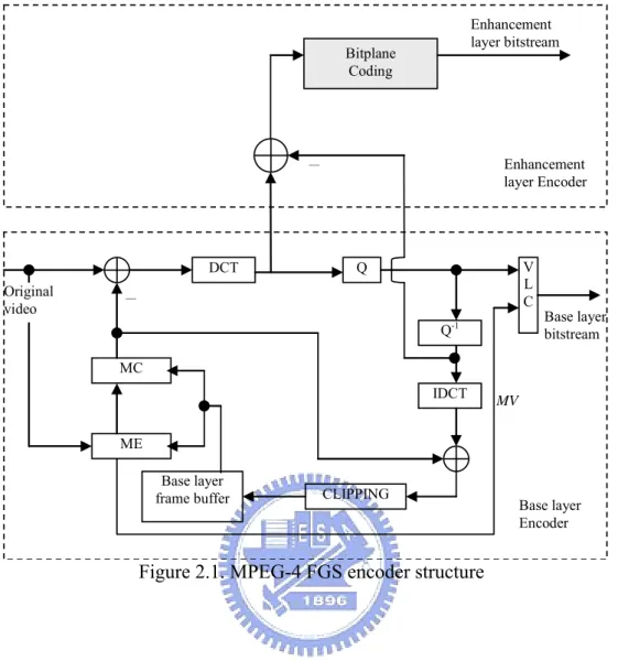
(28) CHAPTER 2 Scalable Video Coding Standard Scalable Video Coding Standard In this chapter, we introduce two scalable video coding standards that related to the thesis. The works of the thesis are originally developed based on the MPEG-4 FGS standard, but can also be used on the H.264/AVC. Recently, the H.264/AVC SVC is developing and has utilized the proposed ideas in this thesis. Both of these two standards are introduced in this section.. 2.1. MPEG-4 FGS. To address the broadcast or Internet multicast applications, the MPEG-4 committee develops the Fine Granularity Scalability (FGS) Profile [6] that provides a scalable approach for streaming video applications. As shown in Figure 2.1, the MPEG-4 FGS representation starts by separating the video frames into two layers with identical spatial resolutions, which are referred to as the base layer and the enhancement layer. The bitstream at base layer is coded by a non-scalable MPEG-4 advanced simple profile (ASP) while the enhancement layer is obtained by coding the difference between the original DCT coefficients and the coarsely quantized base layer coefficients in a bitplane-by-bitplane fashion [10]. The FGS enhancement layer can be truncated at any location, which provides fine granularity of reconstructed video quality proportional to the number of bits actually decoded. There is no temporal prediction for the FGS. - 10 -.
(29) Enhancement layer bitstream. Bitplane Coding. Enhancement layer Encoder. -. DCT Original video. V L C. Q. - Q-1. Base layer bitstream. MC IDCT. MV. ME Base layer frame buffer. CLIPPING. Base layer Encoder. Figure 2.1. MPEG-4 FGS encoder structure. enhancement layer, which provides an inherent robustness for the decoder to recover from any errors. However, the lack of temporal dependency at the FGS enhancement layer decreases the coding efficiency as compared to that of the single layer non-scalable scheme defined in [11].. 2.2. H.264/AVC SVC. 2.2.1 Overview To further improve the coding efficiency of SVC and achieve flexible visual content adaptation for multimedia communications, the ISO/IEC MPEG and ITU-T - 11 -.
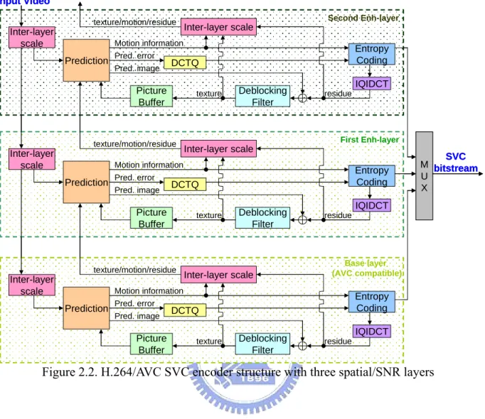
(30) VCEG form the Joint Video Team (JVT) to develop a scalable video coding standard based on the H.264/AVC standard [1][2][3] (referred to as H.264/AVC SVC in the following). The H.264/AVC SVC standard receives worldwide industrial support and will be elevated to Final Draft International Standard in January 2007. The H.264/AVC SVC technology consists of hierarchical-B structure with leaky prediction. To enhance coding efficiency among coding layers, it adopts adaptive inter-layer prediction techniques including intra texture, motion, and residue predictions. The constrained inter-layer prediction is used for reduced decoder complexity. A cyclic block coding is used for SNR scalability with better subjective quality. In this section, we will provide an overview of these technologies and a comparison of coding efficiency between H.264/AVC and H.264/AVC SVC. The rest of this paper is organized as follows: Section 2.2.2 describes the encoder structure of H.264/AVC SVC. Sections 2.2.3 through 2.2.5 examines temporal, SNR, and spatial scalability. Section 2.2.6 and 2.2.7 illustrates the on-going interlaced representation and bit-stream adaptation. Section 2.2.8 compares the coding efficiency between non-scalable H.264/AVC and H.264/AVC SVC. Section 2.2.9 gives a summary of H.264/AVC SVC.. 2.2.2 Overall Encoder Structure. - 12 -.
(31) Input Video texture/motion/residue. Inter-layer scale Prediction. Motion information Pred. error Pred. image. texture. texture/motion/residue. Deblocking Filter. IQIDCT residue. First Enh-layer. Inter-layer scale. Motion information. Prediction. Pred. error Pred. image. Entropy Coding. DCTQ. Picture Buffer. texture/motion/residue. Inter-layer scale. Entropy Coding. DCTQ. Picture Buffer. Inter-layer scale. Second Enh-layer. Inter-layer scale. texture. Deblocking Filter. Inter-layer scale. IQIDCT residue. Base layer (AVC compatible). Motion information Pred. error Prediction DCTQ Pred. image. Picture Buffer. texture. SVC M bitstream U X. Entropy Coding Deblocking Filter. IQIDCT residue. Figure 2.2. H.264/AVC SVC encoder structure with three spatial/SNR layers. In this section, we present an overview of the encoder structure of H.264/AVC SVC. The H.264/AVC SVC encodes the video into multiple spatial, temporal, and SNR layers 1 for combined scalability. Figure 2.2 shows a generic structure of H.264/AVC SVC encoder with three spatial layers (or SNR layers).The input video is spatially decimated to support various spatial resolutions, which is coded with separated encoders as shown in dotted boxes of Figure 2.2.. 1. In this chapter, we use “SNR layer” instead of “quality layer” to indicate the layers at the same resolution but with different quality. This is to prevent the ambiguity with the “quality layer” technique that is used for the bit stream adaptation, which will be described in section 2.2.7.2.. - 13 -.
(32) Key picture Layer 4. 0. 1. 2. H. 3. 4. H L. Layer 3. Key picture. 5. 6. H L. H. 7. 8. H L. 10 11 12 13 14 15 16. H L. H. H L. H L. L. H L. H. L. Layer 2. 9. L. H L. H. L. H L. Layer 1. L. H L. Layer 0. prediction update (a) MCTF prediction structure Key picture Layer 0. Key picture. 0. 16 8. Layer 1. 4. Layer 2. 2. Layer 3 Layer 4. 1. 12 6. 3. 10. 5 7 9 11 (b) Hierarchical-B prediction structure. 14 13. 15. Figure 2.3. Temporal decomposition For each spatial layer, temporal scalability of multiple levels is supported with hierarchical-B structure [4], and motion compensated temporal filtering (MCTF) structure can be used as a pre-processing tool for better coding efficiency. The two. - 14 -.
(33) prediction structures are illustrated in Figure 2.3 and more detail will be given in Section 2.2.3. Since the information of different layers contains correlations, an inter-layer prediction scheme reuses the texture, motion, and prediction information of the lower layers to improve the coding efficiency at the enhancement layer. When each layer has different spatial resolution, the prediction needs to perform interpolation. Note that H.264/AVC SVC also support non-dyadic spatial resolution ratio among spatial layers. After the inter-layer prediction module, the residues of each spatial layer are encoded with either an embedded coder for fine granularity scalability (FGS), or a non-scalable coder for coarse granularity scalability (CGS). However, the entropy coding is restricted to non-scalable mode when it is the first SNR layer of a spatial layer (also refer to as “SNR base layer” in this article). The lower layers do not refer to higher layers for prediction so that the removal of enhancement layers does not affect the decoding of lower layers. In the following Sections, we will describe the detail for temporal, SNR and spatial scalability.. 2.2.3 Temporal Scalability The temporal scalability is implemented with hierarchical B-pictures, while Motion Compensated Temporal Filtering (MCTF) can be used as a pre-processing tool for better coding efficiency.. 2.2.3.1 Motion Compensated Temporal Filtering The MCTF is a temporal decomposition technique that adaptively performs the wavelet decomposition and reconstruction along the motion trajectory using Haar and 5/3 wavelets, which can be implemented with lifting schemes with only one prediction/update step. Particularly, the lifting scheme of 5/3 wavelet is realized by - 15 -.
(34) traditional bi-directional prediction. In Figure 2.3 (a), the layer 4 contains the full resolution and the 5/3 wavelet is used for most predictions. For temporal decomposition, the odd-indexed pictures are predicted from the adjacent even-indexed pictures to produce the high-pass pictures. The even-indexed pictures are updated to generate low-pass pictures using combination of the adjacent high-pass pictures. When the Haar wavelet is selected, the uni-directional prediction is formed. As illustrated in Figure 2.3 (a), the prediction and update path of Picture 3 shown with blue color are removed. Particularly, uni-directional prediction can be either forward or backward prediction. In addition, the selection of uni-/bi-directional prediction (i.e., the selection of Haar and 5/3 wavelet) is adaptive for each block. To remove the temporal redundancy, motion compensation is conducted before the prediction and update steps. For temporal scalability of multiple levels, wavelet decomposition is recursively applied on the low-pass pictures of different layers. Using n decomposition stages, up to n levels of temporal scalability can be achieved. The video of lower frame rate consists of the low-pass pictures at lower layer [5]. The MCTF structure requires memory buffer and coding delay equal to the whole GOP size. To reduce the complexity, some backward prediction/update path can be removed. As illustrated in Figure 2.3, removal of the red (and green) prediction/update path reduces the memory requirement and coding delay to half (or quarter) of the GOP size.. 2.2.3.2 Hierarchical-B Structure In MCTF, the un-compressed pictures are employed for prediction leading to an open-loop control. With such control, the encoder provides better prediction since original pictures has higher quality. However, it causes mismatch error between encoder and decoder in the presence of quantization error. Furthermore, the update step doubles - 16 -.
(35) the complexity and increases memory requirement. To investigate the performance of loop control and justify the complexity increase of the update step, several studies have shown that the closed-loop structure without update step outperforms the open-loop MCTF structure in most of the testing conditions [4]. The update step can be replaced by a simpler noise reduction filter and it can be disabled at decoder side without incurring significant degradation of subjective quality. However, the update step at encoder side does reduce the quality variation of decoded pictures. After these studies, a closed-loop control at encoder side replaces the open-loop control and the update step is now removed from the normative parts. This new temporal decomposition structure is known as “hierarchical-B” or “pyramid-B” prediction structure as shown in Figure 2.3 (b). To support closed-loop encoding, the pictures at lower layers are encoded first such that the pictures at higher layers can refer to the reconstructed pictures at lower layers. Another advantage is that such a prediction scheme is already supported by the syntax of H.264/AVC [1]. To reduce the memory requirement and coding delay, the similar concept used in MCTF can be applied to hierarchical-B structure.. 2.2.3.3 Adaptive Reference Fine Granularity. Scalability In the hierarchical-B structure, the key pictures get temporal prediction only from the base layer of the previously coded key pictures but the non-key pictures include both the base and SNR enhancement layers for temporal prediction. Since the base layer has low bit rate and thus poor quality, the key pictures generally have poor prediction efficiency. To improve coding efficiency, the prediction of key pictures should incorporate the SNR enhancement layers. However, drift occurs as the enhancement layer may be truncated. The same problem also exists in the non-key pictures but the. - 17 -.
(36) hierarchical-B structure significantly constrains the length of the prediction path and propagation of drift. The drift problem of key pictures was also extensively discussed during the development of MPEG-4 FGS [6]. In MPEG-4 FGS, the enhancement layer is only predicted from the base layer with poor quality, leading to poor coding efficiency. Several works employ the enhancement layer for prediction with various drift control mechanism [7][8]. In particular, RFGS [8] uses leaky prediction to improve coding efficiency while constraining drifting errors. The predict data from the enhancement layer is multiplied with a leaky factor, which is smaller than one, in each prediction loop. When the predicted data from the enhancement layer are truncated, the drift is decayed by the leaky factor in each prediction loop leading to 3 to 4 dB improvement [8]. The stack robust FGS (SRFGS) further incorporates multiple prediction loops to improve R-D performance over a wide range of bit rates [9]. In H.264/AVC SVC, the adaptive reference FGS (ARFGS) approach adaptively selects the leaky factor at transform coefficient level for improving the coding efficiency of key pictures. The ARFGS prediction process is performed in the transform domain. For each coefficient at the enhancement layer, the ARFGS reference coefficient is constructed from both the co-located coefficient at the reconstructed base layer and the predicted coefficient at the enhancement layer from the previous frame. Depending on whether the co-located residue at the base layer is zero or not, the ARFGS reference coefficient is set equal to a weighted average of the two sources. After generating the ARFGS reference coefficients, they are inverse transformed to spatial domain to obtain the ARFGS reference block. If all the collocated residues in the base layer are zeros, the derivation of ARFGS reference block is simplified to the weighted average of the two sources in the spatial domain, and the transform domain prediction process is skipped. In addition, the multi-loop prediction in SRFGS is also implemented in H.264/AVC. - 18 -.
(37) SVC. A single enhancement layer loop decoding method can be used to reduce complexity with some degradation of the coding efficiency improvement of multi-loop prediction.. 2.2.4 SNR Scalability The SNR scalability consists of Coarse Grain Scalability (CGS) and Fine Grain Scalability (FGS). The former encodes the transform coefficients in a non-scalable way while the latter can be truncated at any location.. 2.2.4.1 Coarse Grain Scalability (CGS) The CGS layer data can only be decoded as an integral part. Each CGS layer has its own motion information and temporal prediction. There is inter-layer prediction for CGS to re-uses information from the lower layers but it does not require spatial interpolation as all layers have identical resolution. Further, it does not use motion vector refinement (quarter-pel refinement mode) as in spatial scalability.. 2.2.4.2 Fine Grain Scalability (FGS) The FGS layer arranges the transform coefficients as an embedded bit stream which allows truncation at any arbitrary point. The cyclical block coding is proposed to achieve embedded representation. Each FGS layer is coded in two passes: significant and refinement passes. The significant pass first encodes the insignificant coefficients (zeros) in the subordinate FGS layers. Then, the refinement pass refines the significant coefficients with data from -1 to +1. During the significance pass, the transform coefficients are coded in a cyclical, block-interleaved manner. Each coding cycle in a block includes an End-of-Block (EOB) symbol, a Run index (number of consecutive zeros), and a non-zero quantization index. The EOB symbol is coded first to signal. - 19 -.
(38) whether there are non-zero coefficients to be coded in a cycle. Then, the Run index represented by several significance bits further locates the non-zero coefficient. In the refinement pass, the significant coefficients are refined in a subband-by-subband fashion. The significant coefficients of low-frequency subbands are refined before those of high-frequency subbands. With block-interleaved coding order in both coding passes, the decoded video can have more uniform quality when the bit stream of FGS layers is truncated. To further reduce the bit rate, each symbol can be coded by CABAC or CAVLC. In both entropy coding modes, the spatial correlations are employed by constructing the context model. For example, for the coding of a significance bit, the significance status of the co-located coefficients in the neighboring blocks is referred. Besides using differennt entropy coder, each FGS slice (progressive refinement slice or PR slice) provides one more flag (motion_refinement_flag) to select prediction process. When this flag is set to 0, the motion information will not be refined in a FGS slice. The FGS layer simply re-uses the motion information of the previous SNR layer and successively refines the prediction residue of the previous SNR layer. When the flag is set to 1, it has its own motion and the residue is adaptively predicted from the previous SNR layer. The motion refinement provides more than 1 dB gain, which is more noticeable when the base layer is coded at low bit rate or the FGS layers cover a wide range of bit rates. With motion refinement, FGS also provides similar coding efficiency as the CGS.. 2.2.5 Spatial Scalability Similar to the MPEG-2/4 approach, the spatial scalability is achieved by decomposing the original video into spatial pyramid. As shown in Figure 2.2, each spatial layer is coded independently while the motion and temporal prediction are - 20 -.
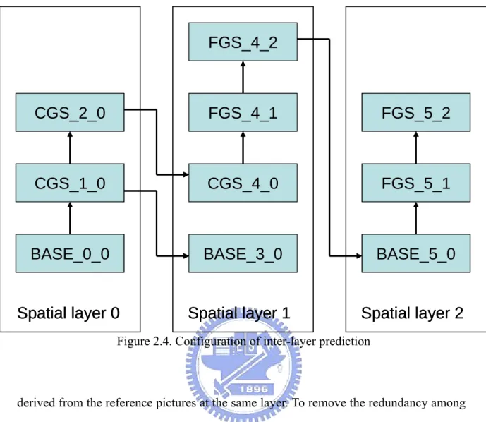
(39) FGS_4_2. CGS_2_0. FGS_4_1. FGS_5_2. CGS_1_0. CGS_4_0. FGS_5_1. BASE_0_0. BASE_3_0. BASE_5_0. Spatial layer 0. Spatial layer 1. Spatial layer 2. Figure 2.4. Configuration of inter-layer prediction. derived from the reference pictures at the same layer. To remove the redundancy among layers, significant inter-layer prediction is used for motion, residue, and texture.. 2.2.5.1 Inter-layer Prediction Structure The inter-layer prediction is dependent on the types of layers used. The spatial and CGS layers can flexibly select the reference layer from any lower layers while the FGS layer must be predicted from the previous SNR layer at the same resolution. As shown with an example in Figure 2.4, each rectangle specifies a coding layer of a picture using the notation of X_Y_Z, where the symbol X denotes coding method of the layer including BASE (the SNR base layer), CGS, and FGS. The second symbol Y and third symbol Z specify the dependency_id and quality_level for a spatial or a SNR layer, where the dependency_id is incremented by 1 for the successive spatial layers or. - 21 -.
(40) CGS layers and the quality_level is incremented by 1 for the successive FGS layers. Both parameters are used by the decoder to identify a coding layer. The BASE_0_0 is the lowest layer that is compatible with H.264/AVC. On top of the BASE_0_0, CGS_1_0 and CGS_2_0 layers are the CGS layers, which are predicted from BASE_0_0 and CGS_1_0, respectively. In the second column, BASE_3_0 is the base layer of the second spatial layer. With flexible selection of the reference layer, BASE_3_0 refers to CGS_1_0 while CGS_4_0 refers to CGS_2_0 instead of BASE_3_0. In this example, CGS_4_0 is decodable even when BASE_3_0 is corrupted by errors. The rule for the FGS layer is different for CGS/spatial layer. The FGS layer can only refer to previous SNR layer of the same resolution. With the configuration shown in Figure 2.4, some layers are redundant for the decoding of certain layer. For instance, the CGS_2_0 is redundant for decoding BASE_3_0. Similarly, BASE_3_0 is redundant for decoding CGS_4_0. Such flexibility is left for further Rate-Distortion performance optimization. The inter-layer prediction information is categorized as intra texture, motion, and residue predictions [3].. 2.2.5.2 Intra Texture Prediction Intra texture prediction uses the reconstructed image of the reference layer to predict an enhancement layer. As the inter-layer prediction of a block refers to an inter-block in the reference layer, or refers to an intra-block in the reference layer that predicted from its neighboring inter-blocks, the motion compensation will be performed at the reference layer to generate the prediction. When multiple spatial layers are coded, such a process may be invoked multiple times leading to significant complexity. To reduce the complexity, the constrained inter-layer prediction is used to allow only intra texture prediction from an intra-block at the reference layer. Moreover, the referred intra-block can only be predicted from another intra blocks (i.e., the reference - 22 -.
(41) layer re-use of “constrained intra prediction” in H.264/AVC). In this way, the motion compensation is invoked only at the highest layer. Such a constraint is also referred to as “single loop decoding”. However, it should be noted that the key pictures can still be configured as multiple loop decoding while the non-key pictures are restricted to the single loop decoding. Before the prediction, the reconstructed image in the reference layer will be firstly de-blocked and spatially interpolated by the 6-tap half-pixel filter.. 2.2.5.3 Motion Prediction Motion prediction is used to remove the redundancy of motion information, including macroblock partition, reference picture index, and motion vector, among layers. In addition to the macroblock modes available in H.264/AVC, H.264/AVC SVC creates two additional modes for the inter-layer motion prediction. The first mode (base layer mode) reuses the motion information of the reference layer without spending extra bits. The second mode (quarter-pel refinement mode) refines the motion vector to quarter-pixel precision. The allowable offset of refinement is -1 or 1. If neither one is selected, independent motion is encoded. Note that the motion vectors and macroblock partition of the reference layer may be interpolated before the prediction.. 2.2.5.4 Residue prediction Residue prediction is used to reduce the energy of residues after temporal prediction. A similar idea was proposed in PFGS [7], where the DCT coefficients of the enhancement layer are predicted from those of the base layer. In H.264/AVC SVC, the residue prediction is performed in spatial domain. Due to the inter-layer motion prediction, consecutive spatial layers may have similar motion information. Thus, the residues of consecutive layers may exhibit strong correlations. However, it is also possible that consecutive layers have independent motion and thus residues of two consecutive layers become uncorrelated. Therefore, the residue prediction in - 23 -.
(42) H.264/AVC SVC is done adaptively at macroblock level. Like the motion prediction, the residues at the reference layer are interpolated with a bilinear filter before the prediction. Spatially, each macroblock is interpolated separately and the filtering process cannot cross the macroblock boundary.. 2.2.6 Interlaced Coding While the H.264/AVC SVC has considered progressive video so far, the interlaced coding tools are necessary when applying the scalability among several common video formats. The H.264/AVC SVC needs to consider a scenario where the base layer is coded with progressive mode while the enhancement layer is coded by interlaced format, and vice versa. Thus, an ad-hoc group (AHG) was established to develop interlaced coding tools for H.264/AVC SVC. However, none of the proposals has been adopted so far. In the following, we briefly summary the techniques that have been proposed for interlaced coding. In the interlaced coding, the main issue for H.264/AVC SVC is the inter-layer prediction since two successive layers may be coded by different modes. Some proposals utilize a “two-steps” approach: one step deals with the inter-layer prediction between different modes (frame or field), but with the same resolution. Another step handles the inter-layer prediction between different resolutions, but with the same mode. The first step is applied on the base layer to generate a “virtual layer” while the second step is applied further on the “virtual layer” to produce the final inter-layer prediction. For example, the inter-layer prediction between a progressive CIF sequence and an interlaced 4CIF sequence is considered. A 4CIF virtual layer is constructed from a progressive CIF and it is followed by the frame to field inter-layer prediction at the same resolution. Due to the possible phase shift of the frame and field between the - 24 -.
數據
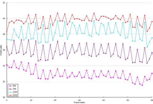
![Figure 3.2. Channel bandwidth variation pattern for the dynamic test defined in the MPEG document m8002 [19]](https://thumb-ap.123doks.com/thumbv2/9libinfo/8224509.170685/53.892.165.688.131.454/figure-channel-bandwidth-variation-pattern-dynamic-defined-document.webp)
+7
Outline
O VERVIEW OF D ISSERTATION
Temporal Scalability
Spatial Scalability
Analysis of Error Propagation
S IMPLIFIED RFGS P REDICTION S CHEME
E XPERIMENT R ESULTS AND A NALYSES
S PATIAL S CALABILITY AND SNR SCALABILITY
F INE G RANULARITY S CALABILITY (FGS)
The Mobile WiMAX Simulation Platform
Simulation results
相關文件
In 2007, results of the analysis carried out by the Laboratory of the Civic and Municipal Affairs Bureau indicated that the quality of the potable water of the distribution
In 2007, results of the analysis carried out by the Laboratory of the Civic and Municipal Affairs Bureau indicated that the quality of the potable water of the distribution
In 2007, results of the analysis carried out by the Laboratory of the Civic and Municipal Affairs Bureau indicated that the quality of the potable water of the distribution
the prediction of protein secondary structure, multi-class protein fold recognition, and the prediction of human signal peptide cleavage sites.. By using similar data, we
Valor acrescentado bruto : Receitas do jogo e dos serviços relacionados menos compras de bens e serviços para venda, menos comissões pagas menos despesas de ofertas a clientes
An information literate person is able to recognise that information processing skills and freedom of information access are pivotal to sustaining the development of a
Wang, Solving pseudomonotone variational inequalities and pseudocon- vex optimization problems using the projection neural network, IEEE Transactions on Neural Networks 17
Define instead the imaginary.. potential, magnetic field, lattice…) Dirac-BdG Hamiltonian:. with small, and matrix
