動態網格之姿勢相依多層精細度模型

國

立

交

通

大

學

資訊工程系

碩

士

論

文

動態網格之姿勢相依多層精細度模型

Pose-Dependent Level of Detail Modeling for Animated Meshes

研究生：呂宗弘

指導教授：莊榮宏 博士

Pose-Dependent Level of Detail Modeling for Animated Meshes

研 究 生：呂宗弘 Student：Zong-Hong Lyu

指導教授：莊榮宏 Advisor：Jung-Hong Chuang

國 立 交 通 大 學

資 訊 工 程 系

碩 士 論 文

Institute of Computer Science and Information Engineering College of Electrical Engineering and Computer Science

National Chiao Tung University in partial Fulfillment of the Requirements

for the Degree of Master in

Computer Science and Information Engineering

October 2005

Hsinchu, Taiwan, Republic of China

中華民國九十四年十月

2 2

Pose-Dependent Level of Detail Modeling for Animated Meshes

Student: Zong-Hong Lyu

Advisor: Dr. Jung-Hong Chuang

Department of Computer Science and Information Engineering

National Chiao Tung University

ABSTRACT

3D animation is now very popular in the movies and games. Since 3D animation in game is usually performed in real-time, complex models created by artist are often simplified to models of low polygon count. While many simplification methods have been proposed for static mod-els, very few methods are available for the deformable meshes. Current simplification methods for deformable meshes are either computationally expensive or incapable of producing satisfac-tory results. In this thesis, we propose an efficient pose-dependent level of detail frame work for deformable meshes. Our approach consists of two stages. The first stage preprocesses all costly computation steps and for each frame generates a simplified mesh using a common vertex hier-archy. The second stage generates in-between meshes between two consecutive key frames via connectivity blending and geometry interpolation. We have observed that the proposed method is able to efficiently generate smooth transition between two pose-dependent meshes, while requiring very little extra data storage.

Keywords: level of detail, mesh simplification, progressive meshes, vertex hierarchy, de-formable mesh, animation.

Acknowledgments

I would like to thank my advisors, Dr. Jung-Hong Chuang, for his inspirations, guidance and patience for the past years.

I also appreciate all my classmates and members of the CGGM laboratory, for their assis-tances and discussions. Especially, thank Tan-Chi Ho for guidance for this thesis.

I am grateful to my mother, father, my brother and my friends for their support, encourage-ment and love.

Contents

2.4 Deformable Model Simplifications . . . 6

2.4.1 Fixed Collapsing Sequence Simplifications . . . 7

2.4.2 Dynamic Connectivity on Deforming Models . . . 8

3 Pose-Dependent Level of Detail Modeling 11 3.1 Approach Overview . . . 11

3.2 Preprocessing . . . 12

3.3 Key Frame Transition . . . 15

4 Experimental Results 21 4.1 Tests on the Preprocessing Stage . . . 25

4.2 Tests of the Key Frame Transition Stage . . . 30

4.3 Experiments Summary . . . 35

5 Conclusion and Future Work 39

5.1 Summary . . . 39 5.2 Future work . . . 39

Bibliography 41

List of Figures

2.1 Edge collapsing and vertex splitting [7]. . . 5

2.2 PM sequence [12]. . . 5

2.3 A TDAG with five time-steps, and the DAGs encoded in it[19]. . . 8

2.4 A changing of parent in the finer level results in edge flip in coarser level [13]. . 9

2.5 The QEM distribution of a vertex during the animation sequence. [10] . . . 10

3.1 Computing the vertex collapsing sequence for a key frame. . . 13

3.2 Determining the mesh connectivity for each key frame. . . 14

3.3 Vertex splits and collapses required for blending. . . 16

3.4 Vertex collapse operation performed in wrong frames may introduce serious visual defect. . . 18

4.1 The animation sequence of M-test model. . . 22

4.2 The horse collapse animation sequence. . . 23

4.3 The camel gallop animation sequence. . . 24

4.4 The simplified meshes for key frames of M-model. . . 26

4.5 Simplified meshes for key frame of horse collapse animation. . . 27

4.6 Simplified meshes for key frames of camel gallop animation. . . 28

4.7 Comparison of the RMS errors for each key frame of horse collapse model. . . 29

4.8 Comparison of the RMS errors for each key frame of camel gallop model. . . . 29

4.9 Comparison on inter frames of our approach and uniformly distributed frames. . 30

4.10 Comparison of the RMS error for different policies on operation allocation for interpolated frames. . . 31

4.11 The key frame transition results for M-test model between two key frames. . . . 32

4.13 RMS error comparison of the horse collapse model for key frame transition stage. 33 4.14 RMS error comparison of the camel gallop model for key frame transition stage. 34 4.15 Number of operations needed between each two key frames. . . 35 4.16 Transition time needed between each two key frames. . . 36

C H A P T E R

1

Introduction

1.1

Motivation

3D animation has been used heavily in the movie and game industry. Except in the movie industry, most 3D animation applications require real-time rendering of the scene. Since models created by artists often contains too many polygons to be rendered in real-time, one common solution is the level-of-detail modeling, aiming to provide appropriate model resolution for real-time rendering.

Many algorithms have been proposed for static models to derive a progressive mesh by using a series of primitive reduction operations such as vertex collapsing [8], edge collapsing [6], or vertex decimation [18], etc. When these algorithms are applied to deformable meshes, it is better to take the geometry of all poses into account. To this end, existing methods fall into two categories. The first category is pose-independent simplification that derives a single error metric from all poses, and generates a single mesh for all key frames using the resultant error metric [3, 9, 15]. These kind of methods suffer from having too less polygons for representing features that only appears in one or two poses, since they can only generate an ”average” mesh for the animation. The second kind of methods change the connectivity of the simplified mesh during the animation sequence [10, 13, 19], but they are usually computationally expensive and thus must be preprocessed, making them work only for fixed animation sequence.

1.2

Contributions

We propose a two-stage pose-dependent level of detail modeling for animated meshes. In the preprocessing stage, a simplified model for each key frame is derived using a common vertex hierarchy, which is built by taking the geometry of all key frame into account. In run-time stage, smooth between meshes are generated from two consecutive key frames. The in-between meshes are obtained by efficient connectivity blending and geometry interpolation. Compared to existing pose-dependent level-of-detail modeling, the proposed method is efficient and applicable to real-time applications, and can be easily integrated into existing animation systems.

1.3

Thesis Organization

In chapter 2 we will introduce background and previous work related to this thesis. Chapter 3 presents our pose-dependent level of detail schemes. In chapter 4 the experimental results will be given, and chapter 5 is the conclusions and discusses of future work.

C H A P T E R

2

Related Work

In this chapter, a review on related works of our method will be given. Section 2.1 intro-duces the general architectures of level of detail (LOD) modeling. In section 2.2, we describe a widely-used presentation of multi-resolution meshes structure called progressive meshes [7]. In section 2.3, we will introduce the method of measuring errors of mesh simplification operations used in our approach. In the last section, we will describe the methods of deformable mesh simplifications.

2.1

Level-of-detail Modeling

Level-of-detail (LOD) modeling aims to represent a complex mesh with several levels of detail. An appropriate level that has least polygon count with acceptable visual error is selected to be rendered at run time to represent the original mesh. Several methods have been proposed in this field. Most methods simplify the given mesh by using series of primitive reduction operations, like edge collapsing [8], triangle collapsing [6], vertex clustering [16], vertex removal [18] and multi-triangulations [4].

These primitive reduction operations can be performed in various orders, but the mostly used algorithms are using greedy methods. Each operation is assigned a cost measured by some kind of error metric, and the operation with the least cost is performed first, followed by operations ordered in increasing costs.

Several error metrics have been proposed to determine the cost of a primitive reduction op-eration, such as quadric error metrics (QEM) [5], appearance-preserving simplification (APS) [11], image-driven simplification (IDS) [14] and perceptually guided simplification of lit,

tured meshes [20]. All these different metrics focus on minimizing different measured errors of different properties of the original mesh. For example, QEM aims to minimize the geometric error on the simplified mesh, and APS aims to minimize the distortion on the texture domain. We will describe the error metric used in our proposed method in section 2.3.

Existing LOD methods can be divided into two category: discrete LOD [2] or continuous

LOD [7]. Discrete LOD creates versions of various level of detail for the original mesh, each

of which has no direct relation to other levels and cannot be derived from other levels. On the other hand, continuous LOD creates a data structure encoding a continuous spectrum of detail so that a mesh with desire level of detail can be extracted from this structure in run time. The progressive meshes is an example of continuous LOD, and will be described in section 2.2.

2.2

Progressive Meshes (PM)

The progressive meshes consists of a base mesh and a sequence of primitive reduction oper-ations used to coarsen the base mesh to represent a multi-resolution triangular mesh. PM is constructed using greedy algorithm by performing a series of primitive reduction of increasing costs on the original mesh, such as vertex collapsing operation, until no reduction operation is possible. First, all possible vertex collapsing operations of the input mesh are collected as candidates, then the cost of each candidate is calculated, and finally the vertex collapsing op-erations are performed in the order of increasing cost. After each vertex collapse, the costs of remaining candidates shall be updated, and operations that become invalid will be removed from the candidate list. A cost updating step maybe time consuming and can be delayed using lazy evaluations, as proposed in [5].

Each vertex collapsing operation removes one vertex and generally two faces from the mesh. And to refine a simplified mesh back to a higher level of detail, series of inverse operations are performed on the mesh in inverse order of the construction sequence. Vertex splitting is the inverse operation of vertex collapsing, which adds a vertex and generally two faces back to the mesh. Figure 2.1 shows the behaviors of a vertex collapsing and vertex splitting.

Given an input mesh M and a sequence of n vertex collapsing operations, a PM sequence with n + 1 levels of detail can be constructed. An example is shown in figure 2.2, where a mesh M5, after five edge collapsing operations, results in a PM of six levels. The mesh of the

simplest level is denoted as M0. The next level of each level can be acquired by performing

2.3 Error Metrics 5

Figure 2.1: Edge collapsing and vertex splitting [7].

Figure 2.2: PM sequence [12].

splitting operation.

2.3

Error Metrics

The cost of a primitive reduction operation like vertex collapse can be approximated by a num-ber of error metrics, such as geometric error metrics (QEM) [5], appearance-preserving simpli-fication [11] and image driven simplisimpli-fication [14]. In this section we will briefly describe QEM, of which a modified version is used as the error metric of our proposed method.

QEM approximates the cost of each vertex collapsing operation as the sum of squared dis-tances from the remaining vertex v to all planes, which contains the original faces that were connected to those vertices collapsed to v. In the original meshes, each vertex can be seen as the solution of the intersection of a set of planes which connected to it. So we can define the sum of squared distances between a vertex and those planes associated to it as following equation:

4(v) = 4([vx, vy, vz, 1]>) =

X

p∈planes(v)

(p>v)2 (2.1) where p = [a, b, c, d]T represents the plane defined by the equation ax + by + cz + d = 0,

4(v) = X p∈planes(v) (v>p)(p>v) = X p∈planes(v) v>(pp>)v = v>( X p∈planes(v) Kp)v (2.2)

where Kpis the 4x4 matrix:

Kp = p>p =         a2 ab ac ad ab b2 _{bc bd} ac bc c2 _cd ad bd cd d2         (2.3)

Now we can define the approximate error of collapsing two vertices v1and v2as the

follow-ing equation:

v>(Q₁+ Q₂)v (2.4) where v is the new vertex position after v1 and v2 collapsed. We also need to propagate the

error metrics to the new vertex when two vertices collapsed. We simply add up the two quadric metric Q1 and Q2 together to propagate the error metric. While some of the planes have been

counted multiple times, every single plane can be counted at most 3 times since each plane is only associated to the 3 vertices of the triangle in the original mesh.

As you can see, the operation cost of a vertex collapsing operation is heavily affected by the new position of vertex v, we can compute the best position for v by solving ∂4/∂x =

∂4/∂y = ∂4/∂z = 0. This is equivalent to solving:         q11 q12 q13 q14 q21 q22 q23 q24 q31 q32 q33 q34 0 0 0 1         v =         0 0 0 1        

where qij = the (i, j)-th element of Qv. If the coefficient matrix is not invertible, we just pick

among the positions of v1, v2or (v1 + v2)/2 that has the least cost.

2.4

Deformable Model Simplifications

Although literatures discussing mesh simplification have been existed for quite some years, the academic community shows interests to the simplification of deformable model only very

2.4 Deformable Model Simplifications 7

recently. The literature by D. Schmalstieg, et al. [17] is the first public document that mentioned some discussions about this issue. Their methods require the user to partition the mesh into deformable and non-deformable regions. Then those deformable parts will be preserved more during the simplification.

In this section, we will describe several approaches that simplifies a deformable model with-out user assistant. These approaches can be divided into two categories. One kind of them use pose-independent approaches to produce a simplified progressive mesh that have fixed connec-tivity during the animation sequence. They do not change the connecconnec-tivity of mesh to better approximate the features of original meshes in different key frame. The other kind of them use pose-dependent approaches which change the connectivity during the animation sequence.

2.4.1

Fixed Collapsing Sequence Simplifications

J. Houle, et al. proposed a frame work to deal with bone-skinned models [9]. But their main issue focus on how to back propagate the transform metrics from the world space back to bone space after a vertex is being collapsed. They use the quadric error metric of a single pose as their error metric; their simplification method does not consider features of different frames.

A. Mohr, et al. proposed a new error metric modified from the original QEM to determine the primitive reduction cost in their works [15]. The initial simplification step in our proposed approach is based on their work. To consider all poses of the deformable mesh, they track one quadric error per vertex for each pose and sum up the vertex contraction cost of each pose. The cost of collapsing v1and v2 becomes

k

X

i=1

vi>(Qi,v1 + Qi,v2)vi (2.5)

where k means the number of sample poses, vimeans the new position of the collapsed vertex at

each pose and Q_i,v1 and Q_i,v2 means the QEM on v1 and v2at each sample pose respectively. If

the cost of a vertex contraction becomes larger at some poses, it will be penalized to be executed later, so those operations who have the average smaller costs will be performed earlier.

The results produced by their proposed error metric is good for general deformable models which can be used in most game or virtual reality applications. But if the model deforms too much, visual defects can be easily noticed.

C. DeCoro, et al. proposed another frame work to deal with linear blend bone-skinned models [3]. The error quadric proposed by their method is also modified from the original QEM,

which encapsulates knowledge of deformations over all poses, in addition to the configurations of the static initial mesh. Their results work quiet good, but is limited to linear blend bone-skinned models.

2.4.2

Dynamic Connectivity on Deforming Models

A. Shamir, et al. designed a scheme for changing connectivity meshes simplification [19]. Time-dependent Directed Acyclic Graph (TDAG) is introduced by merging individual simpli-fication on each frame into a unified graph. TDAG is built by merging the individual multi-resolution hierarchies for each frame of a mesh sequence together into a unified graph. Tags are assigned to each node specifying the time interval over which the node should be alive. The T-DAG has the advantage of being able to handle arbitrary topology changes as well as geometric deformations. But it is hard to track mesh connectivity from the graph, and as the poses number increasing, the storage space needed grows inefficiently. Figure 2.3 shows the basic idea of the TDAG structure.

Figure 2.3: A TDAG with five time-steps, and the DAGs encoded in it[19].

S. Kircher, et al. proposed another frame work to change the connectivity dynamically [13]. The basic idea of their approach is to start from a initial simplification of the first pose, and adjust the mesh during the subsequent poses to minimize the total error in a given pose. They use

swap as the basic operation to refine their mesh connectivity, which is defined as the operation

to change a vertex’s parent vertex to another in the collapsing hierarchy. After a swap operation, the total QEM error of the mesh may change because now a vertex is collapsed to a different vertex. Figure 2.4 shows the effect of the swap operation. It may change the connectivity of

2.4 Deformable Model Simplifications 9

the mesh because a swap in the finer level may cause the edge flipping in the coarser level. They change the mesh connectivity from one pose to another by performing a series of swap operations that can lower the total error of the mesh until no further improvements can be made.

Figure 2.4: A changing of parent in the finer level results in edge flip in coarser level [13].

The results of this approach is generally good even if the model deforms dramatically. But the refinement process from one pose to another is too local, means that non-necessary oper-ations may be performed. And when the level of detail is low, the computation cost of the refinement process to propagate the geometry errors between different levels becomes too large to be done in real time.

F.C. Huan, et al. proposed another approach similar to the Kircher’s approach [10], but they simplify each pose of the model separately. They also use QEM as their error estimating metric, but they apply wavelet quantization to the distribution of the error cost of each vertex (See Fig-ure 2.5 for an example, the blue line indicates the original error cost, and the red line shows the result after apply wavelet quantization.). This results in a more averagely distributed error cost so additional connectivity will be preserved a few frames before and after the featured frame. They use vertex split and collapse as the basic operations to change the mesh connectivity, and dynamical programming and genetic algorithm is used to find the optimize operation sequence to change the mesh connectivity from one frame to the next frame.

This approach generate simplified meshes that will refine the featured region several frames earlier than the actual featured frames, and coarsen that region several frames later after the featured frames past. The major drawback is that this methods is very slow, so it can only be used on animation sequences that can be known before replay, and can only be preprocessed.

C H A P T E R

3

Pose-Dependent Level of

Detail Modeling

3.1

Approach Overview

Existing pose-independent LOD methods generate static meshes that may fail to properly ap-proximate animated meshes [3, 9, 15, 17]. Those who change the connectivity during the animation sequence are, however, too costly to be done in run time, meaning that they can only work on fixed animation sequence [10, 13, 19]. The approach we proposed is pose-dependent, but efficient enough to be applied in real-time applications.

We divide our approach into two parts: the preprocessing stage which results in meshes with different connectivity but sharing same vertex hierarchy and the key frame transition stage to transit the connectivity and geometry smoothly between key frames. The purpose of the preprocessing stage is to construct a common vertex collapsing hierarchy tree for all key frame meshes, and then compute the vertex collapsing sequence for each key frame, base on the hierarchy. Using the collapsing sequences and the vertex collapsing hierarchy the connectivity of the simplified mesh at a given level can be achieved quickly.

The key frame transition stage generates a series of meshes between two key frames to smoothly transform the model from one pose to another. This stage can be integrated into exist-ing key frame animation system, dynamically changexist-ing the connectivity of the simplified mesh, and interpolating the geometry between key frames. Since the results of the preprocessing stage share the same vertex hierarchy, connectivity blending and geometry interpolation can be done quickly. If the key frame animation sequence are fixed, this stage could also be preprocessed to

further decrease the overhead in the animation system.

3.2

Preprocessing

Since a simplified mesh with fixed connectivity cannot properly represent a deformed mesh, and those methods that change the connectivity during animation sequence are too complex for real-time rendering, the main goal of the preprocessing stage is to produce simplified meshes that have different connectivity, but share a common vertex hierarchy for all key frames.

Two steps are involved in this stage. First, a common vertex collapsing hierarchy is con-structed from the initial simplification step. Then, the vertex collapsing sequence for each key frame is derived. To build a common vertex hierarchy, an initial simplification that considers the geometry of all key frames is performed. We use the metric proposed by Mohr and Gleicher [15] and edge collapsing as our basic operation to do the initial simplification. The metric is a modified version of the original QEM [5], aiming to consider all key frames. The cost of collapsing v1 to v2 using geometry of all key frames becomes

k

X

i=1

vT₂(Qi,v1 + Qi,v2)v2 (3.1)

where k is the number of key frames and Qi,v1 and Qi,v2 represent the QEM values on v1 and

v2 for key frame i, respectively. We initialize the QEM on each vertex at each key frame, then

sum up the QEM of two vertices when they are collapsed to one vertex.

Based on this sequence, a common vertex hierarchy tree for all key frames can be con-structed, where all of the leaf nodes are the original vertices, and each inner node represents an edge collapsing operation by their two child vertices. The left child node of a parent is collapsed and the right child node is the remaining vertex after collapsing; the parent node and its right child node represents the same vertex.

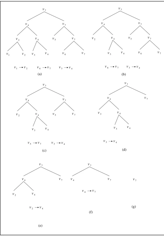
Based on the vertex hierarchy, the edge collapsing sequence for each key frame is com-puted. The procedure is very similar to the original QEM method except that the candidate edge collapses are limited to the edge collapsing that is used to derive the vertex hierarchy. The simplification priority queue is initialized with all of leaf nodes of the tree that can immediately be collapsed to another vertex, and the QEM values of all leaf nodes are computed using the vertex position setting in that key frame. The edge with smallest QEM value in the priority queue is selected as the candidate to be collapsed. As one edge collapse is performed, the ver-tex which is being collapsed to will be checked if it is available for such an edge collapse ; if

3.2 Preprocessing 13 1 v 2 v v5 7 v 7 v 4 v v6 4 v 7 v 4 v 7 v 2 v v3 1 v v2 v6 v7 v3 v4 (a) 2 v v5 7 v 7 v 4 v v6 4 v 7 v 4 v 7 v 3 v 6 v v7 v3 v4 (b) 2 v v5 v7 4 v 4 v 7 v 4 v 7 v 3 v 3 v v₄ 5 v v7 (c) 2 v 4 v 4 v 7 v 4 v 7 v 3 v 3 v v₄ (d) 2 v v4 7 v 4 v 7 v 2 v v4 (e) 7 v 4 v 7 v 4 v v7 (f) 7 v (g)

Figure 3.1: Computing the vertex collapsing sequence for a key frame.

not, we should wait until it becomes available.

1 v 2 v v₃ 3 v 5 v 7 v 7 v 4 v v6 4 v 7 v 4 v 7 v 1 v 2 v v3 3 v 5 v 7 v 7 v 4 v v₆ 4 v 7 v 4 v 7 v ① ② ③ ④ ⑤ ⑥ ④ ⑥ ⑥ ⑦ ⑦ ⑦ ⑦ 1 v 2 v v3 3 v 5 v 7 v 7 v 4 v v₆ 4 v 7 v 4 v 7 v ① ② ② ③ ④ ⑤ ⑥ ⑦ ⑥ ⑥ ⑦ ⑦ ⑦

Figure 3.2: Determining the mesh connectivity for each key frame.

in each step are listed below each figure. Figure 3.1(a) shows the states in initial step. From 3.1(b) - (g) show step by step how this procedure works. Note in Figure 3.1(b), vertex v2

cannot be put into the priority queue because v4is unable to be collapsed up to now, and will be

collapsed until step in Figure 3.1(d) is performed, then v2 can be collapsed to v4. The similar

situations also occurred at step in Figure 3.1(c).

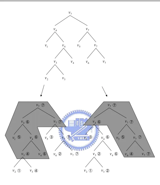
To obtain the given simplification level quickly, we record a vertex collapsing number for each vertex as the order in the collapsing sequence for each key frame. To obtain a given

simpli-3.3 Key Frame Transition 15

fication level of detail of the mesh on a given key frame, we use the vertex collapsing numbers to determine a cut on the hierarchy; if the vertex collapsing number of an edge collapsing is less than the current level number, then it is collapsed, otherwise it will be in the simplified mesh. A triangle of the original mesh exists in the simplified mesh if it did not degenerates (that is it has no two or more vertices collapsed to the same vertex). Figure 3.2 shows an example of deter-mining the mesh connectivity for a given level number. The top figure shows the original vertex hierarchy. The lower figures are cuts for two key frames having different collapsing order given the level number = 4. The grey parts of the figures represent all vertices that are not collapsed.

The procedure for the preprocessing stage can be summarized as the following steps:

• Perform an initial simplification to obtain an edge collapsing sequence and construct the

corresponding vertex hierarchy.

• Based on the hierarchy, compute the vertex collapsing number for each vertex for each

key frame.

The common hierarchy, the collapsing number and the collapsing cost of each vertex on each key frame are saved for the next stage, to quickly obtain the simplified mesh of a given level on each key frame. The transition between two key frame mesh will be describe in the next section.

3.3

Key Frame Transition

For two consecutive key frames, key frame animation system generates in-between meshes by interpolating meshes for key frames. Since our simplified meshes for key frames have different connectivity, we need to blend the connectivity between two key frames as the mesh transform form one key frame to another. Furthermore, the error of the interpolated meshes between two key frames should be minimized. Our algorithm uses some kind of greedy methods based on the collapsing cost stored on the vertices in each key frame to achieve this goal. By using the common vertex hierarchy and stored vertex collapsing number from the previous stage, these transitions can be done efficiently.

First we explain how the geometry interpolation is performed in our system. Because we have common vertex hierarchy for each key frame, the vertex positions of interpolated meshes between two key frames can be interpolated from the corresponding vertices of the two key

frames. We have no limitation on what kinds of interpolation methods that can be used to interpolate the vertex positions.

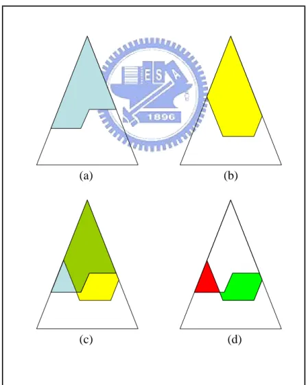
The connectivity transition between the simplified meshes for key frame i to i + 1 can be described by a series of vertex splits and vertex collapses. We first list all operations required to blend the connectivity from key frame i to i + 1 by comparing the active cuts for these two key frames. Nodes that exist in the active cut for key frame i, but not in active cut for key frame i + 1 should be collapsed, otherwise nodes that do not appear in active cut for key frame

i but in active cut for key frame i + 1 should be split. Figure 3.3 illustrates the process to find

all required operations, where Figure 3.3(a) shows the cut of the hierarchy in key frame i and Figure 3.3(b) shows the cut in key frame i + 1. Figure 3.3(c) shows the comparison of the two key frames and Figure 3.3(d) shows the final results in which vertices included in the red region should be collapsed and vertices in the green region will be split.

(a) (b)

(c) (d)

Figure 3.3: Vertex splits and collapses required for blending.

These operations are then put into two priority queues based on the cost of the operations; one for the split operations and the other one for the collapse operations. The reason to use two

3.3 Key Frame Transition 17

priority queues is that we want to keep the polygon count of the simplified mesh as a constant value, so a vertex split operation execution should be followed by an edge collapse operation, and vice versa.

The cost of a vertex split or an edge collapse operation is defined as the difference between the QEM errors of the same vertex or edge on two key frames. So the cost of collapsing v1 to

v2becomes

(v₂T(Qi,v1+ Qi,v2)v2) − (vT2(Qi+1,v1 + Qi+1,v2)v2) (3.2)

where Qi,v1 and Qi,v2represent the QEM of vertex v1and v2for key frame i, Qi+1,v1 and Qi+1,v2

represent the QEM of vertex v1and v2 for key frame i + 1.

Base on the observation that if the error of an operation is smaller in key frame i but greater in key frame i + 1, then this operation should be executed in the frames closer key frame i to decrease the visual popping effect and minimize the error; on the other hand, if the error is smaller in key frame i + 1, this operation should be executed in the frames near to key frame

i + 1. Figure 3.4 depicts the potential error introduced by an operation performed in different

frames. In the left part of the figure, an edge collapse is performed while its cost is small, there will be no trivial visual popping effect. But in the right part of the figure, the cost for the edge collapsing is large; serious visual defect will be noticed.

The operations in the two priority queues will be executed along with the vertex positions interpolation; at each frame the vertex positions are computed while we change the connectivity between two subsequence frames. We can use any methods of existing animation systems to interpolate the vertex positions, because they deal with geometry properties only while our system changes the connectivity of the mesh.

We can do these operations averagely during the transformation between two key frames, but to minimize the error of the interpolated mesh and popping effect caused by vertex split or collapse operations, a bound value is computed for each frame to determine between which two frames an operation should be done. The bound value of a frame is defined as

boundi = (mincost ∗ (n − i) + maxcost ∗ i)/n (3.3)

where n represents the number of frames to transform the mesh from one key frame to the other,

i indicates the frame’s order where i should be 0 at the previous key frame and be n at the next

key frame, mincost and maxcost are the minimum and maximum cost of the operations in the priority queues, respectively.

Figure 3.4: Vertex collapse operation performed in wrong frames may introduce serious visual defect.

We decide when to do an operation by comparing the bound values of these frames. If an operation’s cost sits between the bounds of two subsequence frames, it should be executed between these two frames, because we want to minimize the visual popping effect and to keep the geometry errors as lower as possible. In fact, The geometry errors during the key frame transition process would be minimized if we do all operations with negative costs right between the previous key frame and the first frame interpolated, and do those with positive costs just between the last frame interpolated and the next key frame. It is because the operations with negative costs mean that their error grows as the mesh transforms from the previous key frame to the next, so the earlier it is executed, the smaller error it would cause. For the operations with positive costs the similar argument explains why the should be executed later. But to load balance between these frames and minimize visual popping effect (too many operations executed between two frames will cause serious popping effect), the bound value approach is proposed to spread these operations during the key frame transition.

Finally, if the animation sequence is fixed, we could preprocess this stage to further decrease the overhead by storing the operations between each key frame and between which two frames these operations should be executed. Then during the animation play process, all we need to do

3.3 Key Frame Transition 19

is executing the operations between the two frames recorded to change the connectivity. The algorithm of this stage is given below to summarize this section:

• List all operations needed to change the mesh connectivity from the previous key frame

to the next.

• Put these operations into two priority queues which one is for split operations and the

other is for collapse operations.

• During the frame transition process, execute these operations according the bound values

C H A P T E R

4

Experimental Results

In this chapter, experimental results of our work will be given. We will compare the errors measured on results of our work obtained by using different policies on operation allocation for interpolated frame. Then we will test and compare the errors measured on results of proposed method with a method using fixed connectivity. Finally, the performance in the key frame transition stage of proposed work will be given.

All tests in this chapter are performed on a PC with Intel(R) Pentium(R) 1.3G CPU and 256MB of RAMS.

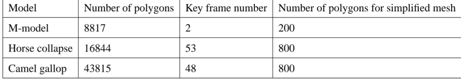
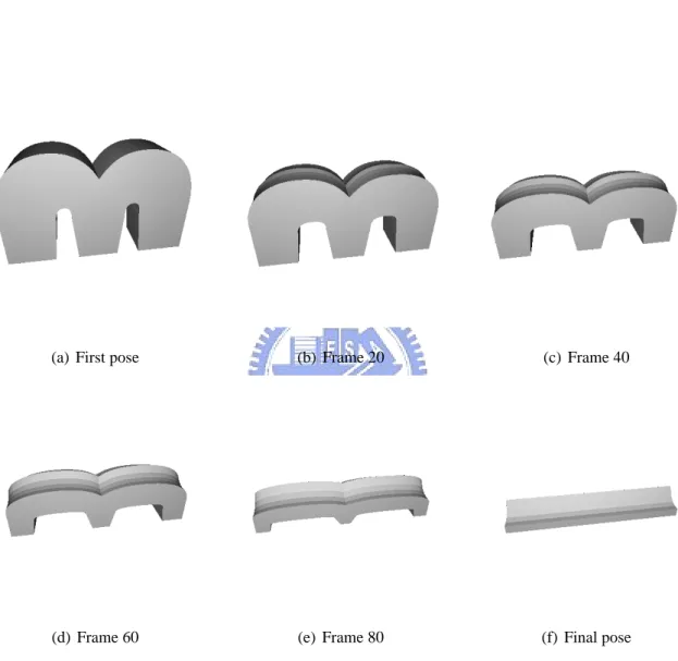
Animation models used in the testing include M-model morphing sequence with 2 key frames as shown in Figure 4.1, a horse collapse animation sequence with 53 key frames as shown in Figure 4.2, and a camel gallop animation sequence with 48 key frames as shown in Figure 4.3. Table 4.1 lists the data of models used in our experiments.

To measure the difference between the simplified model and the original one, we use the root mean square (RMS) error between the original model and the simplified one measured by the Metro tool [1]. In the following contexts, RMS is used to denote the root mean square error between the original mesh and the simplified mesh measured by the Metro tool.

Model Number of polygons Key frame number Number of polygons for simplified mesh

M-model 8817 2 200

Horse collapse 16844 53 800

Camel gallop 43815 48 800

Table 4.1: Models used in our tests.

(a) First pose (b) Frame 20 (c) Frame 40

(d) Frame 60 (e) Frame 80 (f) Final pose

23

(a) Key frame 1 (b) Key frame 11 (c) Key frame 21

(d) Key frame 32 (e) Key frame 42 (f) Key frame 53

(a) Key frame 1 (b) Key frame 9 (c) Key frame 17

(d) Key frame 25 (e) Key frame 33 (f) Key frame 41

4.1 Tests on the Preprocessing Stage 25

4.1

Tests on the Preprocessing Stage

The preprocessing stage of our approach generates simplified meshes at each key frame with different connectivity but using the same vertex hierarchy, so it should be better than those methods that generate simplified meshes with fixed connectivity. We compare our results with the works of A. Mohr, et al. [15] because their method generates good results on a general deformable model. We also compare the RMS error of our work with the results by using QEM metric to directly simplify the mesh.

The simplified meshes of M-model for 2 key frames are shown in Figure 4.4, and the RMS errors of proposed approach , Mohr’s approach, and QEM that considers each individual key frame are shown in Table 4.2. Because the model deforms a lot between the two key frames, our method generates better result. The horse collapse model is another case that deforms dra-matically during the animation sequence. Figure 4.5 shows the simplified meshes for some of the key frames, and Figure 4.7 shows the results of RMS errors comparison between proposed method, Mohr’s method, and direct QEM. The simplified meshes of camel gallop model com-pared with Mohr’s work is shown in Figure 4.6. The results of RMS errors comparison is shown in Figure 4.8. There are several key frames that the RMS errors of our method become greater then Mohr’s work. This is because that a model with smaller a QEM error does not mean that it should have a smaller RMS error, since QEM approximates error only on the vertices, and Metro samples over all of the meshes. The differences here is also very small to be distinguished by human eyes.

Key Frame RMS of proposed method RMS of Mohr’s method RMS of direct QEM

1 0.167959 0.178115 0.041192

2 0.12155 0.195316 0.000000

(a) Key frame 1 (proposed method) (b) Key frame 1 (Mohr’s method)

(c) Key frame 2 (proposed method) (d) Key frame 2 (Mohr’s method)

4.1 Tests on the Preprocessing Stage 27

(a) Key frame 1 (proposed method) (b) Key frame 11 (proposed method) (c) Key frame 21 (proposed method)

(d) Key frame 1 (Mohr’s method) (e) Key frame 11 (Mohr’s method) (f) Key frame 21 (Mohr’s method)

(g) Key frame 32 (proposed method) (h) Key frame 42 (proposed method) (i) Key frame 53 (proposed method)

(j) Key frame 32 (Mohr’s method) (k) Key frame 42 (Mohr’s method) (l) Key frame 53 (Mohr’s method)

(a) Key frame 1 (proposed method) (b) Key frame 9 (proposed method) (c) Key frame 17 (proposed method)

(d) Key frame 1 (Mohr’s method) (e) Key frame 9 (Mohr’s method) (f) Key frame 17 (Mohr’s method)

(g) Key frame 25 (proposed method) (h) Key frame 33 (proposed method) (i) Key frame 41 (proposed method)

(j) Key frame 25 (Mohr’s method) (k) Key frame 33 (Mohr’s method) (l) Key frame 41 (Mohr’s method)

4.1 Tests on the Preprocessing Stage 29 0 0.2 0.4 0.6 0.8 1 1.2 1 3 5 7 9 11 13 15 17 19 21 23 25 27 29 31 33 35 37 39 41 43 45 47 49 51 Frame RMS MY RMS FIX RMS QEM RMS

Figure 4.7: Comparison of the RMS errors for each key frame of horse collapse model.

0 0.0005 0.001 0.0015 0.002 0.0025 0.003 0.0035 1 3 5 7 9 11 13 15 17 19 21 23 25 27 29 31 33 35 37 39 41 43 45 47 Frame MY RMS FIX RMS QEM RMS

4.2

Tests of the Key Frame Transition Stage

4.2.1

Tests of Different Policies on Operation Allocation for Interpolated

Frame

The M-model is used in tests of this subsection shown in Figure 4.1. The number of frames used from key frame 1 to key frame 2 is 100. The polygon count of the simplified meshes is 200.

A bound value is used in each interpolated frame to determine which operations should be performed for this frame. We compare the results for the approach without using the bound and performing the operations uniformly distributed among the transition frames. Figure 4.9 shows the 60-th frames during the transition from key frame 1 to key frame 2. As can be observed, the featured parts are collapsed earlier in the uniformly distributed approach.

The RMS error comparing to original mesh is shown in Figure 4.10. The error of our approach stays low during the entire transition while there are several peaks in the approach using uniformly distributed frames.

(a) The 60-th frame using our approach. (b) The same frame using uniformly distributed frames.

4.2 Tests of the Key Frame Transition Stage 31 0 0.1 0.2 0.3 0.4 0.5 0.6 1 5 9 13 17 21 25 29 33 37 41 45 49 53 57 61 65 69 73 77 81 85 89 93 97 Frame RMS MY RMS AVG RMS

Figure 4.10: Comparison of the RMS error for different policies on operation allocation for interpolated frames.

4.2.2

Results of the Key Frame Transition Stage

In this subsection, we show the key frame transition results of the simplified testing models and compare with the works of A. Mohr, et al.

The results of key frame transition between simplified models are shown in Figure 4.11, and the results of RMS errors comparison between proposed work and Mohr’s work are shown in Figure 4.12. Compared with Mohr’s work, our approach have lower RMS errors during the entire transition session.

The RMS comparison results for horse collapse animation sequence are shown in Figure 4.13. And Figure 4.14 shows the RMS comparison results of the camel gallop animation se-quence. We can observe that the RMS error values of the in-between frames is generally smaller than the values by linear interpolating the two values of the two key frames. And this means the frame transition between two key frames is performed smoothly in our proposed method.

(a) Key frame 1 (proposed method) (b) Frame 20 (proposed method) (c) Frame 40 (proposed method

(d) Key frame 1 (Mohr’s method) (e) Frame 20 (Mohr’s method) (f) Frame 40 (Mohr’s method)

(g) Frame 60 (proposed method) (h) Frame 80 (proposed method) (i) Key frame 2 (proposed method)

(j) Frame 60 (Mohr’s method) (k) Frame 80 (Mohr’s method) (l) Key frame 2 (Mohr’s method)

4.2 Tests of the Key Frame Transition Stage 33 0 0.05 0.1 0.15 0.2 0.25 0.3 1 5 9 13 17 21 25 29 33 37 41 45 49 53 57 61 65 69 73 77 81 85 89 93 97 Frame RMS MY RMS FIX RMS

Figure 4.12: RMS error comparison of the M-model between proposed work and Mohr’s work for key frame transition stage.

0.8 0.82 0.84 0.86 0.88 0.9 0.92 0.94 0.96 0.98 1 Key frame 1 2 3 4 5 6 7 8 9 10 11 12 13 14 15 16 17 18 19 20 21 22 23 24 25 26 27 28 29 30 31 32 33 34 35 36 37 38 39 40 41 42 43 44 45 46 47 48 49 50 51 Frame RMS MY RMS FIX RMS

0.0027 0.0028 0.0029 0.003 0.0031 0.0032 0.0033 Key frame 1 2 3 4 5 6 7 8 9 10 11 12 13 14 15 16 17 18 19 20 21 22 23 24 25 26 27 28 29 30 31 32 33 34 35 36 37 38 39 40 41 42 43 44 45 46 Frame RMS MY RMS FIX RMS

4.3 Experiments Summary 35

4.3

Experiments Summary

As can be seen in the test results of previous sections, our approach performs much better than pose-independent approach, even when the animated model deforms greatly. The overhead of our approach to the animation system is the cost for changing the connectivity between two key frames, which is determined by the number of operations performed. In our implementation, a vertex split or collapse operation cost less than 0.1 ms, and only tens of operations are needed for each connectivity blending from one key frame to another. In general, this amount of overhead can be ignored. In Table 4.3, the number of operations and transition time required for horse collapse model to transit between key frames is given. Figure 4.15 and Figure 4.16 show the statistic for the number of operations and transition time required between each two key frames, respectively. The two peaks in Figure 4.16 are caused by system performing other routines.

0 5 10 15 20 25 1 ~ 2 3 ~ 4 5 ~ 6 7 ~ 8 9 ~ 10 11 ~ 12 13 ~ 14 15 ~ 16 17 ~ 18 19 ~ 20 21 ~ 22 23 ~ 24 25 ~ 26 27 ~ 28 29 ~ 30 31 ~ 32 33 ~ 34 35 ~ 36 37 ~ 38 39 ~ 40 41 ~ 42 43 ~ 44 45 ~ 46 47 ~ 48 49 ~ 50 51 ~ 52

0 0.2 0.4 0.6 0.8 1 1.2 1 ~ 2 3 ~ 4 5 ~ 6 7 ~ 8 9 ~ 10 11 ~ 12 13 ~ 14 15 ~ 16 17 ~ 18 19 ~ 20 21 ~ 22 23 ~ 24 25 ~ 26 27 ~ 28 29 ~ 30 31 ~ 32 33 ~ 34 35 ~ 36 37 ~ 38 39 ~ 40 41 ~ 42 43 ~ 44 45 ~ 46 47 ~ 48 49 ~ 50 51 ~ 52

4.3 Experiments Summary 37

Between which two frames Number of operations Transition time in ms

1 - 2 2 0.173765101 2 - 3 2 0.172088911 3 - 4 2 0.168736529 4 - 5 4 0.229638124 5 - 6 6 0.255898445 6 - 7 6 0.270984161 7 - 8 6 0.250869873 8 - 9 6 0.233549236 9 - 10 6 0.256457175 10 - 11 10 0.293612736 11 - 12 4 0.23159368 12 - 13 12 0.331327026 13 - 14 6 0.236342887 14 - 15 6 0.224888917 15 - 16 8 0.293612736 16 - 17 8 0.26707305 17 - 18 6 0.267352415 18 - 19 6 0.235784157 19 - 20 6 0.986158855 20 - 21 4 0.22991749 21 - 22 4 0.227961934 22 - 23 12 0.386641319 23 - 24 14 0.380774652 24 - 25 14 0.398095289 25 - 26 16 0.455923867 26 - 27 20 0.468215932 27 - 28 12 0.347809568 28 - 29 16 0.432177833 29 - 30 16 0.384685763

Table 4.3: Number of operations and transition time needed of the horse collapse model. Con-tinued in Table 4.4.

Between which two frames Number of operations Transition time in ms 30 - 31 20 0.480507998 31 - 32 16 0.363174649 32 - 33 12 0.334958773 33 - 34 14 0.385803224 34 - 35 12 0.357866712 35 - 36 14 0.322107977 36 - 37 14 0.344457187 37 - 38 8 0.273219082 38 - 39 12 0.325180994 39 - 40 12 0.285231782 40 - 41 8 0.275733368 41 - 42 8 0.260368287 42 - 43 8 0.240533364 43 - 44 8 0.241371459 44 - 45 10 0.285511147 45 - 46 10 0.248355587 46 - 47 6 0.22013971 47 - 48 10 0.714336599 48 - 49 8 0.297523847 49 - 50 14 0.357587347 50 - 51 12 0.311771468 51 - 52 10 0.285511147 52 - 53 8 0.309574681

C H A P T E R

5

Conclusion and Future Work

5.1

Summary

In this thesis, we have proposed a two-stage approach to simplify a deformable model based on the key frames. The inter frames between each key frame is interpolated in our system to transform the mesh from a key frame to another smoothly.

The first stage performs preprocessing steps, which generates a simplified mesh for each key frame with different connectivity, but sharing a common vertex collapsing hierarchy. The hierarchy is constructed by considering all poses of the key frames, and the simplified mesh of each key frame is generated by considering the error metric of the specified key frame, which results in better approximation to the original mesh for this key frame.

The second stage performs key frame transition to transform the mesh from key frame i to i + 1 smoothly by connectivity blending and geometry interpolation. We list all operations needed in the transition stage and order them by consider the costs of the operations in the two key frames. To decide in which frame an operation should be performed, a bound value is computed in each key frame. The results of the generated inter frames is generally good for common deformable models.

5.2

Future work

The vertex hierarchy is constructed based on the works of A. Mohr, et al. [15]. Maybe there are better metrics that can be used in this step, like the metric of C. DeCoro, et al. [3]

In some of our test models, like the m-test model, the common vertex hierarchy has

bidden us to further improve the simplified mesh for some key frames. So another possible improvement is to break the limitation caused by using a common hierarchy to construct the simplified mesh for each key frame. Maybe we can use a method similar to the work proposed by S. Kircher, et al. [13] to change the hierarchy in the preprocessing stage and encode these operations to be used in the second stage.

In the key frame transition stage, a bound value is used to decide when an operation should be performed. This is some kind of heuristic, and may generate bad results sometimes. Better mechanics maybe used to further reduce the visual popping effects and mesh geometry errors.

And our work does not take texture coordinates into consideration during the simplification process. Because most animation applications use models with texture, an extension of our works can be done to consider the texture coordinates distortion in the simplification process.

Bibliography

[1] P. Cignoni, C. Rocchini, and R. Scopigno. Metro: Measuring error on sim-plified surfaces. Computer Graphics Forum, 17(2):167–174, 1998. URL

http://vcg.iei.pi.cnr.it/metro.html.

[2] J. H. Clark. Hierarchical geometric models for visible surface algorithms. In

Communi-cations of the ACM, volume 19(10), pages 547–554, 1976.

[3] C. DeCoro and S. Rusinkiewicz. Pose-independent simplification of articulated meshes. In Proceedings of ACM Symposium on Interactive 3D Graphics, pages 17–24, Apr. 03–06 2005.

[4] L. D. Floriani, P. Magillo, and E. Puppo. Efficient implementation of multi-triangulations. In Proceedings of IEEE conference on Visualization ’98, pages 45–50, 1998.

[5] M. Garland and P. S. Heckbert. Surface simplification using quadric error metrics. In

Proceedings of ACM SIGGRAPH, pages 209–216, Aug. 1997.

[6] B. Hamann. A data reduction scheme for triangulated surfaces. In Computer Aided

Geo-metric Design, volume 11, pages 45–50, 1998.

[7] H. Hoppe. Progressive meshes. In Proceedings of ACM SIGGRAPH, pages 99–108, Aug. 1996.

[8] H. Hoppe, T. DeRose, T. Duchamp, J. McDonald, and W. Stuetzle. Mesh optimization. In

Proceedings of ACM SIGGRAPH, pages 19–26, 1993.

[9] J. Houle and P. Poulin. Simplification and real-time smooth transitions of articulated meshes. In No description on Graphics interface, pages 55–60, June 07–09 2001.

[10] F.-C. Huang, B.-Y. Chen, Y.-Y. Chuang, and M. Ouhyoung. Animation model simplifica-tions. In Computer Graphics Workshop, Nov. 2005.

[11] M. O. Jonathan Cohen and D. Manocha. Appearance-preserving simplification. In

Pro-ceedings of ACM SIGGRAPH, 1998.

[12] J. Kim and S. Lee. Transitive mesh space of a progressive mesh. In IEEE Transaction on

Visualization and Computer Graphics, pages 463–480, Dec. 2003.

[13] S. Kircher and M. Garland. Progressive multiresolution meshes for deforming surfaces. In Proceedings of ACM SIGGRAPH/Eurographics symposium on Computer animation, pages 191–200, July 29–31 2005.

[14] Lindstrom and G. Turk. Image-driven simplification. In ACM Transactions on Graphics, 2000.

[15] A. Mohr and M. Gleicher. Deformation sensitive decimation. In University of Wisconsin

Technical Report, Apr. 2003.

[16] J. Rossignac and P. Borrel. Multi-resolution 3d approximations for rendering complex scenes. In Modeling in Computer Graphics: Methods and Applications, pages 455–465, 1993.

[17] D. Schmalstieg and A. Fuhrmann. Coarse view-dependent levels of detail for hierarchical and deformable models. Technical Report TR-186-2-99-20, Institute of Computer Graph-ics and Algorithms, Vienna University of Technology, Favoritenstrasse 9-11/186, A-1040 Vienna, Austria, sep 1999. human contact: [email protected].

[18] W. J. Schroeder, J. A. Zarge, and W. E. Lorensen. Decimation of triangle meshes. In ACM

SIGGRAPH Computer Graphics, volume 26(2), pages 65–70, July 1992.

[19] A. Shamir, V. Pascucci, and C. Bajaj. Multi-resolution dynamic meshes with arbitrary deformations. In Proceedings of IEEE conference on Visualization, pages 423–430, 2000.

[20] N. Williams, D. Luebke, J. D. Cohen, M. Kelley, and B. Schubert. Perceptually guided simplification of lit, textured meshes. In Symposium on Interactive 3D Graphics, 2003.