Contents lists available atSciVerse ScienceDirect
Neural Networks
journal homepage:www.elsevier.com/locate/neunet
2013 Special Issue
Single-hidden-layer feed-forward quantum neural network based on
Grover learning
Cheng-Yi Liu
a,b, Chein Chen
a, Ching-Ter Chang
c, Lun-Min Shih
d,∗ aDepartment of Computer Science, National Chiao Tung University, 1001 University Road, Hsinchu 300, Taiwan bDepartment of Information Management, TransWorld University, 1221 Zhennan Road, Douliu, Yunlin 640, Taiwan cDepartment of Information Management, Chang Gung University, 259 Wen-Hwa 1st Road, Kwei-Shan, Taoyuan 333, Taiwan dDepartment of Accounting Information, DaYeh University, 168 University Road, Changhua 515, Taiwanh i g h l i g h t s
• A single-hidden-layer quantum neural network is proposed.
• Our model is proposed based on some concepts and principles in the quantum theory. • Grover learning is presented for training the network.
• Some experiments are taken to compare the proposed method with other SLFNNs.
a r t i c l e i n f o Keywords: Neural network Quantum computing Grover algorithm
a b s t r a c t
In this paper, a novel single-hidden-layer feed-forward quantum neural network model is proposed based on some concepts and principles in the quantum theory. By combining the quantum mechanism with the feed-forward neural network, we defined quantum hidden neurons and connected quantum weights, and used them as the fundamental information processing unit in a single-hidden-layer feed-forward neural network. The quantum neurons make a wide range of nonlinear functions serve as the activation functions in the hidden layer of the network, and the Grover searching algorithm outstands the optimal parameter setting iteratively and thus makes very efficient neural network learning possible. The quantum neuron and weights, along with a Grover searching algorithm based learning, result in a novel and efficient neural network characteristic of reduced network, high efficient training and prospect application in future. Some simulations are taken to investigate the performance of the proposed quantum network and the result show that it can achieve accurate learning.
© 2013 Elsevier Ltd. All rights reserved.
1. Introduction
In the past seventy years, artificial neural networks (ANNs) have made rapid developments and been successfully applied into a great deal of practical scientific and engineering problems (Bishop,
1995;Hastie, Tibshirani, & Friedman, 2001;Haykin,1994). Feed-forward neural networks (FNNs) and recurrent neural networks (RNNs) are two major types of popular artificial neural networks. The single-hidden-layer feed-forward neural network (SLFNN) is one of the most widely used ANNs, which have no lateral con-nections and/or cyclic concon-nections and whose features resort to parameters of the weighted connections and hidden nodes ( Er-dogmus, Fontenla-Romero, Principe, Alonso-Betanzos, & Castillo, 2005;Huang, Chen, & Siew, 2006;Huang, Zhu, & Siew, 2006;Kim
∗Corresponding author. Tel.: +886 937237596. E-mail address:[email protected](L.-M. Shih).
& Adali, 2003;Liang, Huang, Saratchandran, & Sundararajan, 2006). Modification of these adjustable parameters in the ANNs allows the network to learn an arbitrary vector mapping from the space of inputs to the outputs. Finding an approximate set of parameters which can minimize the defined performance function is often re-alized by iterative learning. However, this process is very tedious and the optimization result relies heavily on the learning algorithm and the complexity of performance function. Moreover, the classi-cal feed-forward neural networks are also facing many difficulties, including the dimensionality calamity, the determination of the best architecture, the limited memory capacity, time-consuming training, and so on.
In recent years there has been an explosion of interest in quan-tum computing. Quanquan-tum processing allows the solution of an op-timization problem through the exhaustive search undertaken on all the possible solutions of the problem itself, and now it has been applied to several scientific fields such as physics, math-ematics, and an extension to the entire field of computational 0893-6080/$ – see front matter©2013 Elsevier Ltd. All rights reserved.
intelligence (Ezhov & Ventura, 2000;Fiasché,2012;Friedman, Pa-tel, Chen, Tolpygo, & Lukens, 2000;Gupta & Zia, 2001;Han, Gao, Su, & Nie, 2001;Han & Kim, 2002;Kak,1995;Narayanan & Menneer, 2000;Panella & Martinelli, 2007;Perkowski,2005;Platel, Schliebs, & Kasabov, 2009). Nowadays several essential ideas in the quantum computing have formed the basis for researches of quantum intelli-gent computing, including the linear superposition, entanglement and so on.
Linear superposition is closely related to the familiar mathe-matical linear combination. The basis of linear superposition state, and in general the superposition coefficient of the state is complex. Entangled quantum system is the potential to show the classical correlation. From a computing point of view, entanglement seems to be intuitive enough. In fact, the existence of quantum superpo-sition makes the correlation exist. When the consistency lost, the communication correlation is probably between the qubits in some way.
Recently there have been growing interests in ANNs based on some concepts and principles in quantum theory (Ezhov & Ventura, 2000;Gupta & Zia, 2001;Kak,1995;Narayanan & Menneer, 2000;
Panella & Martinelli, 2007;Perkowski,2005). The quantum system lays a foundation of the microcosmic systems for all the physical process, including the biologic process and mental process. Several works have combined the quantum computing with the traditional evolution algorithms that simulate the biological evolution (Fiasché,2012;Han & Kim, 2002;Platel et al.,2009). So the quantum system is more suitable for the description of the complex biological evolution as well as the biological neurons.
Combining quantum computing with training and implemen-tation of neural networks has been studied by many researches (Ababneh & Qasaimeh, 2006; Ezhov & Ventura, 2000; Fiasché,
2012;Friedman et al.,2000;Gupta & Zia, 2001;Han et al.,2001;
Han & Kim, 2002;Kak,1995;Karayiannis et al.,2006;Kretzschmar, Bueler, Karayiannis, & Eggimann, 1996;Levy & McGill, 1993; Mal-ossini, Blanzieri, & Calarco, 2008; Narayanan & Menneer, 2000;
Narayanna & Moore, 1996;Panella & Martinelli, 2007;Patel,2001;
Perkowski,2005;Platel et al.,2009;Purushothaman & Karayiannis, 1997). In 1997, Quantum neural network with multi-level activa-tion funcactiva-tion is firstly proposed by Karayiannis, which uses quan-tum ideas superposition in the quanquan-tum theory (Bishop,1995;
Haykin,1994). The multi-stage activation function in the network is a linear activation Sigmoid function in the hidden layer of QNN, which is the so-called superposition. Each Sigmoid function has a different quantum interval. By adjusting the Quantum interval, the data can be mapped to different spaces that are determined by the quantum level. Given appropriate training algorithm, the network can adaptively extract the inner rules even if class boundaries or re-gression functions are blurred. Therefore, in the classification task, if the feature vector in the boundary between the classes overlap, QNN will be assigned to all classes (Bandyopadhyay, Karahaliloglu, Balkir, & Pramanik, 2005; Barbosa, Vellasco, Pacheco, Bruno, & Camerini, 2000;Hou,2011;Mukherjee, Chowdhury, Raka, & Bhat-tacharyya, 2011;Qiao & Ruda, 1999a, 1999b;Takahashi, Kurokawa, & Hashimoto, 2011;Xuan,2011). Therefore, the multi-quantum level of activation is the key reason that QNN can solve fuzzy clas-sification and regression effectively (Gao, Zhang, Liu, Chen, & Ni, 2010;Guowei, Ning, & Deyou, 2010;Huifang & Mo, 2010;Ji, Liu, Yu, & Wu, 2011;Li & Xu, 2009;Liu, Peng, & Yang, 2010;Sagheer & Metwally, 2010;Xianwen, Feng, Lingfeng, & Xianwen, 2010;Yan & Xia, 2010).
In this paper, we establish a quantum neuron and weights based feed-forward neural network model, single hidden layer feed-forward quantum neural network (SLFQNN), and propose a Grover learning algorithm based on the quantum parallelism and entanglement. The activation function of quantum neurons in the hidden layer is characteristic of quantum coherence and quantum
transition, whose type is not fixed. The coherent coefficient can be adjusted according to the problems to be solved, and a Grover based quantum learning algorithm is used to train the network for a fast and accurate learning. Some simple examples are also given to prove its superiority.
The rest of this paper is organized as follows. Section2 intro-duces the single-hidden-layer feed-forward quantum neural net-work. In Section3, the Grover based quantum learning is explained in detail. In Section4, some experiments are taken to investigate the performance of our proposed method by comparing it with other related methods. The conclusions are finally summarized in Section5.
2. Single-hidden-layer feed-forward quantum neural network (SLFQNN)
In a real human brain, there are many different kinds of neu-rons that process different information. In quantum computation, a quantum state can be looked as a superposition of many ground states. Inspired by it, we take quantum hidden neurons in SLFNN, which is in a state of quantum superposition that is a combina-tion of many ground states. The method of superposicombina-tion can be described by the amplitude of quantum probability and the posi-tion of quantum jump. For an explicit understanding of the quan-tum system, firstly we have a presentation on the quanquan-tum theory.
2.1. Quantum bits
Information is stored in the smallest unit in the two state quan-tum computer is called a quanquan-tum bit or qubit. A qubit is in the two dimensional Hilbert complex unit vector. For the purposes of Quantum computing, the ground state
|
0⟩
and|
1⟩
represent the classical bit values 0 and 1. However, unlike classical bits, a qubit can in the superposition of state|
0⟩
and|
1⟩
.In a quantum system, the quantum state is the carrier of infor-mation, and a quantum state
|
Ψ⟩
can be regarded as a superpo-sition of many ground states (Kak,1995;Narayanan & Menneer, 2000):|
Ψ⟩ =
N
n=1 Cn|
n⟩
N
n=1|
Cn|
2=
1
,
(1)with
|
n⟩
is the ground state with corresponding coefficient Cn, whose amplitude is the appear probability of the state|
n⟩
. Given an m-bit quantum system:
α 1 β1
α2 β2
· · · · · ·
αm βm
, where|
α
i|
2+ |
β
i|
2=
1(
i=
1,
2, . . . ,
m)
, it can represent the superposition of states and a 3-bit quantum system is:
1 √ 2 1 √ 2
√ 3 2 1 2
1 2 √ 3 2
. So the states ofthis system are:
√ 3 4 √ 2
|
000⟩ +
3 4 √ 2|
001⟩ +
1 4 √ 2|
010⟩ +
√ 3 4 √ 2|
011⟩
+
√ 3 4√2|
100⟩ +
3 4√2|
101⟩ +
1 4√2|
110⟩ +
√ 3 4√2|
111⟩
. There-sult above means the appear probabilities of the states
|
100⟩
,
|
101⟩
, |
110⟩
, |
111⟩
, |
000⟩
, |
001⟩
, |
010⟩
, |
011⟩
are 323,
329,
321,
323,
3 32,
9 32,
1 32,
332 respectively, i.e., we can get the information of 8
states from a 3-qubit system. Additionally, along with the conver-gence of the quantum chromosomes, the diversity fade away and the algorithm converges.
Similar to the quantum state
|
Ψ⟩
, the neuron in human brain is just in such a quantum superposition and accordingly we call it quantum neuron. This quantum neuron has such an activation functionf¯
(
N,
C,
x)
(Friedman et al., 2000):¯
f(
N,
C,
x) =
1 N N
n=1|
Cn|
2fn(
x−
∆n).
(2)Fig. 1. The model of quantum neuron.
Here fn
(
x) (
n=
1, . . . ,
N)
is a nonlinear basis function. Ac-cording to the quantum mechanics of biological brain neuron, the activation function of artificial neurons can be associated to the so-lution of basic such as Schroedinger’s equation for various types of external potential. If the external potential is zero or constant then such basis functions will be Gaussian functions; if the external po-tential is harmonic such basis functions will be Hermite functions; moreover, a Morlet wavelet basis function can also be expanded by a spectral superposition of Gaussian basis functions. For other types of wavelet functions, the probability density functions asso-ciated to quantum mechanical equations can be approximated by wavelet expansions, however, these expansions do not coincide with the mathematical solutions of the associated partial differ-ential equations. So in the formula(2)the admissible neuron ac-tivation function f(
x)
can be radial Gaussian function, or Wavelets functions, x is the input data. They are corresponding to the quan-tum ground states at different energy levels, and∆nis the quan-tum transition position of these states. Accordingly, the output of quantum neuron¯
f(·)
will be in a superposition state that is formed by these ground states. The model of quantum neuron is shown inFig. 1.
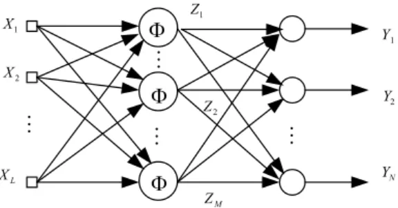
2.2. Quantum neural network
By adopting the quantum neurons as the hidden neurons of a SLFNN, we can establish a SLFQNN. Assume the connected weights in the output layer are represented by W
,
g is the activationfunction of the hidden layer (often a classical linear function is adopted), there is a hidden neuron in SLFQNN, so the output of the network is y
=
g(
W, ¯
f(
N,
C,
x))
(Haykin, 1994). Here N is the number of ground states of quantum neurons; C is the amplitude of appear probability of states in quantum neuron. According to the result of Kreinovich in 1991, a nonlinear function in the hidden layer can make SLFNN approximate any continuous function on the condition of a weak limitation (Kreinovich, Vazquez, & Kosheleva, 1991), so SLFQNN can be proved to have generalized approxima-tion ability. In the training, by adjusting|
Cn|
2, we can get optimal activation functions of hidden layer in SLFQNN by the subsequent learning.3. Grover based quantum learning
In comparison with the classical hidden neurons in ANNs, SLFQNN has two new parameters: the superposition coefficient and the jump position. Assume an SLFQNN with the structure
Li
−
1−
Lo, if the number of the training samples is P and the number of the ground states is N. Firstly we define such a cost function J (Bishop, 1995): J=
1 2 P
i=1 e2i=
1 2 P
i=1 Lo
j=1(
yi,j−
di,j)
2 (3)Fig. 2. The quantum neural network.
where yi,jis the output of the j-th neuron for the i-th training sample: yi,j
=
g(
W, ¯
f(
N,
C,
x))
=
1 N M
l=1|
Dl|
2w
lj N
n=1|
Cn|
2fn(
xi−
∆n)
(
i=
1, . . . ,
P,
j=
1, . . . ,
Lo),
(4) and di,jis the corresponding expected output,w
jis the connected weights between the j-th output neuron and the hidden neu-ron. Searching for an approximate set of parameters including the weights W and the undetermined parameters in quantum neuron, including the quantum superposition state fnand quantum transi-tion∆nin the possible solution space to minimize the cost function is the goal of training the network.Assume the type of quantum neuron is coded with l1
=
log2(
N)
qubits, the transition of quantum neuron is coded with l2
=
log2
(
Q)
and quantum weights W are coded with l3=
log2(
M)
quantum bits. Unlike classical bits, qubits are in the superposition of states
|
0⟩
and|
1⟩
. At some time, the type of hidden quantum neuron is in the superposition state (Panella & Martinelli, 2007):|
ψ⟩ =
√
1 N N
n=1|
fn⟩;
(5)and the transition of the hidden neuron is also in such a superpo-sition state:
|
ϕ⟩ =
√
1 Q Q
n=1|
∆n⟩
.
(6)The quantum weights are in the state:
|
W⟩ =
√
1 M M
k=1|
w
k⟩
(7)which is the superposition of all possible states
w
k∈ [
0,
1, . . . ,
2l3−
1]
, and each state is corresponding to a determined weights. Con-sider a database of S elements exactly one of which is ‘‘marked’’ as satisfying some desirable characteristic, Grover’s algorithm uses the parallelism of afforded by quantum superposition to accom-plish the task with only O(
S1/2)
queries (Liu et al., 2010). In thispaper, we introduce the quantum Grover algorithm to search for the optimal weights and neurons that can maximize the defined performance function. The network is shown inFig. 2.
Defining 1
/
J as the performance function of the network:F
(
W,
f,
∆) =
1/
J.
(8)Grover searching algorithm is to compute the performance func-tion of different states in parallel and search the best parameter set with the highest performance function. Firstly define a
|
q⟩
withl1
+
l2+
l3quantum bits, which is in a combination state of|
ψ⟩, |ϕ⟩
the control register to control the appearance of the optimal state and the obtained
|
q⟩
is of length n=
l1+
l2+
l3+
b:|
q⟩ : |
ψ, ϕ,
W,
c⟩
.
The process of searching for the solution that maximizes the per-formance function can be described as the following steps. First, represent the performance function F as:
F
(
W,
f,
∆) =
F(
q1,
q2, . . . ,
qn).
(9) Define the unity quantum operation U as (Trugenberger, 2002):U
=
exp
iπ
2Fnor(
q1, . . . ,
qn)
(10) with Fnor(
q1, . . . ,
qn) =
F(
q1, . . . ,
qn) −
Fmin Fmax−
Fmin.
(11) Here Fmax,
Fminrepresent the upper and lower bound of theperfor-mance function respectively. Perform the unity quantum operation
U on the state
|
q⟩
: U=
l1+l2+l3
k=1 Gk (12)where Gkis the k-bit diagonals quantum gate as follows (Grover, 1997):
Gk
=
diag(
ei·π2Fnork (01,...,0k), . . . ,
ei·π2Fnork (11,...,1k))
(13)Fnork
(
q1, . . . ,
qk) =
F(
q1, . . . ,
qk) −
K1Fmin Fmax−
Fmin
K=
l1+l2+l3
k=1 k!
n k
.
(14)Firstly the b control bits in
|
q⟩
are initialized as all zeros:|
q0⟩ =
√
1 n n
k=1(
qk:
01, . . . ,
0b).
(15)Perform the Hadamard gate H
=
√1 2
1 1 1 −1
on the first control bit, we can obtain:
|
q1⟩ =
√
1 2n n
k=1(
qk:
01, . . . ,
0b)
+
√
1 2n n
k=1(
qk:
11, . . . ,
0b).
(16) Introduce the control gate (Trugenberger, 2002):Ucq±
= |
1c⟩⟨
1c| ⊗
Uq+ |
0c⟩⟨
0c| ⊗
Uq−1 (17) which represent that if the control bit takes ‘‘1’’, perform unity op-eration U on the state|
qt⟩
; if the control bit takes ‘‘0’’, then performU−1on the state
|
qi⟩
, which can be realized by employing the con-trol gate: Ucq±=
m
k=1(
CGk−2)
Gk.
(18)Perform Uc±1qon
|
q2⟩
, we can obtain,|
q2⟩ =
√
1 2n n
k=1 e−i π2Fnor(qk)|
q k:
01, . . . ,
0b⟩
+
√
1 2n n
k=1 ei π2Fnor(qk)|
q k:
11, . . . ,
0b⟩
.
(19)Apply the Hadamard gate H on the first control bit c1, we can
obtain,
|
q3⟩ =
√
1 n n
k=1 sin
π
2Fnor(
qk)
|
qk:
01, . . . ,
0b⟩
+
√
1 n n
k=1 cos
π
2Fnor(
qk)
|
qk:
11, . . . ,
0b⟩
.
(20)So performing the transform HcUcq±Hc can fulfill the performance function estimation of
|
q⟩
, and consequently we perform such a transform on each control bit C1, . . . ,
Cb, and finally we get the result (Trugenberger, 2002):|
qpf⟩ =
√
1 n n
k=1 b
i=0 cosb−i
π
2Fnor(
qk)
×
sini
π
2Fnor(
qk)
{Ji}|
qk:
Ji⟩
(21)where
{
Ji}
represent the length of binary string with i ‘‘zero’’ andb
−
i ‘‘1’’. In this procedure, b times of operation HcUcq±Hcis used to amplify the probability amplitude of the state with higher per-formance function. The state with highest perper-formance function should have a lot of zero control bit. When all the bits in the control register being in zero, the amplitude of the optimal state reaches the maximum. Commonly speaking, the required state can be obtained by repeatedly performing the above determined quan-tum transformation and random quanquan-tum measurements. The ex-pected iterative times needed to obtain the optimal state is 1/
Pb0, and Pb0=
1 n n
k=1 sin2b
π
2Fnor(
qk)
(22)is the probability of
|
c1, . . . ,
cb⟩ = |
01, . . . ,
0b⟩
. Once the control register detects the desired state, the measurement can be per-formed on|
q⟩
, and then we can obtain the state|
qk⟩
with the proba-bility Pb(
qk)
. We can see from it that with the Fnor(
qk)
approaches 1,Pb
(
qk)
becomes bigger and bigger. Finally, as we have expected, Pb achieves the maximum at the state with the highest performance function.So the Grover based quantum learning algorithm can be de-scribed as:
The procedure of the Grover based learning algorithm: Step 1: Initialize the parameters of the network:
|
q⟩ : |
q1,
q2, . . . ,
ql1,
q1,
q2, . . . ,
ql2,
q1,
q2, . . . ,
ql3,
c1,
c2, . . . ,
cb⟩
where
|
q1,
q2, . . . ,
ql1⟩
code the type of quantum neuron;|
q1,
q2, . . . ,
ql2⟩
code the transition of quantum neuron;|
q1,
q2, . . . ,
ql3⟩
code the connection weights of output layer and|
c1,
c2, . . . ,
cb⟩
are the control bits. The c1, . . . ,
cbcontrol bits in|
q⟩
are initialized as all zeros:Step 2: Defining 1
/
J as the performance function of thenetwork, and perform the unity quantum operation U on the state
|
q⟩
.Step 3: Perform the quantum transform HcUcq±Hcon the coding bits and control bits to estimate the performance function of the states. Repeat this process for Pb0times.
Step 4: Perform the observation on the quantum neuron and
weights, which will collapse into one state, and it is the best state having the highest performance function.
Table 1
The probability of falling into a local optimal solution. Length of b Length of l1,l2,l3 R=Flocal max/Fglobal max
R R=0.2000 R=0.500 R=0.800 R=1.000 b=1 2 0.500 0.452 0.250 0.048 3 0.354 0.320 0.177 0.034 4 0.125 0.226 0.063 0.024 b=2 2 0.500 0.409 0.125 0.005 3 0.354 0.289 0.088 0.003 4 0.125 0.205 0.063 0.002 b=3 2 0.500 0.370 0.063 4.354e−004 3 0.354 0.262 0.044 3.078e−004 4 0.125 0.185 0.031 2.177e−004
Fig. 3. The function to be approx.
4. Experimental results
In this section, some experiments are taken to investigate the performance of the proposed method.
Experiment 1. In the following, a simple example is used to illus-trate the efficiency of the proposed Grover quantum learning al-gorithm. Firstly we investigate the probability of Grover algorithm based quantum learning falling into a local optimal solution. The result is shown inTable 1. From it we can see that when the num-ber of control bits reaches 3 and the information bits reaches 4, the possibility of falling into a local optimal solution becomes very small. So as long as the bits are defined in
|
q⟩
, Grover based quan-tum learning is feasible.Experiment 2. Considering the problem of the function approxi-mation, the function to be approximated is
y
(
x) =
sin x+
sin 3x3
−
2 sinx
2
.
(23)The function is shown inFig. 3.
In SLFQNN Gaussian function is adopted as the fundamental ac-tivation function of the network. The difference among different
fnrelies on the width of Gaussian function, and the transition∆n reflects the centers of Gaussian function. Let l1
=
l2=
l3=
4and b
=
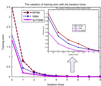
3. BP-NN model is a feed forward neural network with the learning rule of error back propagation. It has a three-layer (or single-hidden-layer) network structure: the input layer, hid-den layer and the output layer. In the network, the parameters of the network are tuned using the traditional gradient descent algo-rithm. It provides a possible way of finding an approximated opti-mal solution to the network parameters and is very popular in theFig. 4. The convergence curves of BPNN, WNN and SLFQNN.
practical application of ANNs. It is also a representative neural net-work model that has the activation functions with global support. WNN is an improved version of the BP-NN, which replace the Sig-moid function in the hidden layer by a local and multiscale wavelet function, followed by a linear output layer. In the training process of the network, the parameters are also adjusted by the traditional gradient descent algorithm, including the connected weights of the network, the scale and position of the hidden neurons. Because the local property of wavelet functions in time and frequency, WNN is more efficient than BP-NN in approximating and classifi-cation tasks. It proves to present good results in many engineering fields. Therefore we compare these two networks with our pro-posed SLFQNN. In this experiment, BP-NN, WNN and SLFQNN are used to approximate the function in(21). In the training, the initial weight and neuron parameters are selected randomly. The SLFQNN network is trained according to the algorithm above.
The result shows that BPNN (Backpropagation neural network), SLFQNN and WNN (wavelet neural network) all can converge within eight epochs to reach the error below 0.01. The SLFQNN converges rapider than BPNN and WNN, as shown inFig. 4. How-ever, for SLFQNN, it only requires four iterations to reach the error 1.3741e
−
3. Additionally the classical neural network needs more hidden neurons to obtain a satisfactory solution, however, only one hidden neuron is employed in our proposed SLQFNN.Experiment 3. In this test, we applied it to the task of classifi-cation, and the data is fromhttp://www.research.att.com/∼yann/
ocr/mnistin AT&T Bell laboratory in America. The number of test samples is 1000, and N
=
3. Moreover, two binary classification datasets came from UCI dataset: Bld (Bupa Liver Disorders), TttTable 2
Result of classification.
Dataset # training samples RBF NN SLFQNN
Error Lh Error Lh
AT&T Bell
100 2.4 72 2.0 1
196 1.8 127 1.8 4
289 1.1 206 0.9 10
Bld (Bupa Liver Disorders) 400 5.2 143 4.1 7
Ttt (tic-tac-toe endgame) 300 5.9 221 4.4 8
(tic-tac-toe endgame) are also used to test the proposed method. RBFNN is a popular single-hidden-layer feed-forward neural net-work that takes the radial-basis-function as the activation func-tion in the hidden layer. The activafunc-tion funcfunc-tion has the multiscale characteristics and it is considered as a special case of the WNN. Different with WNN, RBFNN calculates the distance between the input pattern and the centers in the hidden layer. Because the cen-ters of the hidden neurons can be determined by some supervised clustering algorithm, the training of RNFNN is rapider than that of WNN. In the experiment, we compare the proposed SLFQNN with RBFNN, which uses the Gaussian function as the activation func-tion in the hidden layer and works well in funcfunc-tion fitting, and the result is shown inTable 2. Here Lhrepresents the number of hidden layer. From it we can see that the classical neural network needs a great deal of hidden neurons to obtain a satisfactory solution, how-ever, only a small number of hidden neurons are needed to reach the same precision in SLFQNN.
5. Conclusions
In this paper, a single hidden layer feedforward quantum neural network is proposed based on the combination of quantum the-ory and neural network. In the network, the hidden neurons are quantum neurons that are characteristic of the superposition and transition of multiple states, which can produce a wide range of nonlinear activation functions in the hidden layer of the network. Moreover, the Grover searching algorithm is proposed to outstand the optimal parameter setting iteratively and thus makes very ef-ficient neural network learning possible. The quantum neuron and weights, along with a Grover searching algorithm based learning, result in a novel and efficient neural network characteristic of re-duced network, high efficient training and prospect application in future.
References
Ababneh, J. I., & Qasaimeh, O. (2006). Simple model for quantum-dot semiconductor optical amplifiers using artificial neural networks. IEEE Transactions on Electron Devices, 53(7), 1543–1550.
Bandyopadhyay, S., Karahaliloglu, K., Balkir, S., & Pramanik, S. (2005). Compu-tational paradigm for nanoelectronics: self-assembled quantum dot cellular neural networks. IEE Proceedings—Circuits, Devices and Systems, 152(2), 85–92. Barbosa, C. Hall, Vellasco, M., Pacheco, M. A., Bruno, A. C., & Camerini, C. S. (2000).
Nondestructive evaluation of steel structures using a superconducting quan-tum interference device magnetometer and a neural network system. Review of Scientific Instruments, 71(10), 3806–3815.
Bishop, C. (1995). Neural networks for pattern recognition. Oxford: Oxford Univ. Press. Erdogmus, D., Fontenla-Romero, O., Principe, J. C., Alonso-Betanzos, A., & Castillo, E. (2005). Linear-least-squares initialization of multilayer perceptrons through backpropagation of the desired response. IEEE Transactions on Neural Networks, 16(2), 325–337.
Ezhov, A. A., & Ventura, D. (2000). Quantum neural networks. In N. Kasabov (Ed.), Future directions for intelligent systems and information sciences (pp. 213–234). Berlin, Germany: Springer-Verlag.
Fiasché, M. (2012). A quantum-inspired evolutionary algorithm for optimization numerical problems. In LNCS: Vol. 7665. ICONIP 2012, Part III (pp. 686–693). (Part 3).
Friedman, J. R., Patel, V. V., Chen, W., Tolpygo, S. K., & Lukens, J. E. (2000). Quantum superposition of distinct macroscopic states. Nature, 406(6791), 43–46.
Gao, Kim, Zhang, Yan, Liu, Ying-hui, Chen, Xiao-mei, & Ni, Guo-qiang (2010). PSF estimation for Gaussian image blur using back-propagation quantum neural network. In 2010 IEEE 10th international conference on signal processing, ICSP. (pp. 1068–1073). 24–28 October.
Grover, L. K. (1997). Grover searching algorithm. Physical Review Letters, 79, 325. Guowei, Cai, Ning, Liu, & Deyou, Yang (2010). The transformer fault diagnosis based
on quantum neural network. In T2010 International conference on computer, mechatronics, control and electronic engineering, Vol. 4, CMCE. (pp. 396–400). 24–26 August.
Gupta, S., & Zia, R. K. P. (2001). Quantum neural networks. Journal of Computer and System Sciences, 63, 355–383.
Han, M., Gao, X., Su, J. Z., & Nie, S. (2001). Quantum-dot-tagged microbeads for mul-tiplexed optical coding of biomolecules. Nature Biotechnology, 19(7), 631–635. Han, K. H., & Kim, J. H. (2002). Quantum-inspired evolutionary algorithm for a class
of combinatorial optimization. IEEE Transactions on Evolutionary Computation, 6(6), 580–593.
Hastie, T., Tibshirani, R., & Friedman, J. (2001). The elements of statistical learning: data mining, inference and prediction. Springer.
Haykin, S. (1994). Neural networks: a comprehensive foundation. New York: Macmil-lan.
Hou, Xuan (2011). Research of model of quantum learning vector quantization neural network. In 2011 International conference on electronic and mechanical engineering and information technology, Vol. 8, EMEIT. (pp. 3893–3896). 12–14 August.
Huang, G.-B., Chen, L., & Siew, C.-K. (2006). Universal approximation using incre-mental constructive feed-forward networks with random hidden nodes. IEEE Transactions on Neural Networks, 17(4), 879–892.
Huang, G.-B., Zhu, Q.-Y., & Siew, C.-K. (2006). Real-time learning capability of neural networks. IEEE Transactions on Neural Networks, 17(4), 863–878.
Huifang, Li, & Mo, Li (2010). A new method of image compression based on quan-tum neural network. In 2010 International conference of information science and management engineering, Vol. 1, ISME. (pp. 567–570). 7–8 August.
Ji, Xiao, Liu, Yawen, Yu, Xiaowei, & Wu, Jiangbin (2011). Alternative combination of quantum immune algorithm and back propagation neural network. In 2011 Seventh international conference on natural computation, Vol. 1, ICNC. (pp. 66–70). 26–28 July.
Kak, S. C. (1995). Quantum neural computing. Advances in Imaging and Electron Physics, 94, 259–314.
Karayiannis, N. B., Mukherjee, A., Glover, J. R., Frost, J. D., Hrachovy, R. A., Jr., & Mizrahi, E. M. (2006). An evaluation of quantum neural networks in the detection of epileptic seizures in the neonatal electroencephalogram. Soft Computing, 10(4), 382–396.
Kim, T., & Adali, T. (2003). Approximation by fully complex multilayer perceptrons. Neural Computation, 15, 1641–1666.
Kreinovich, V., Vazquez, A., & Kosheleva, O. (1991). Prediction problem in quantum mechanics is intractable (NP-hard). International Journal of Theoretical, 30(2), 113–122.
Kretzschmar, R., Bueler, R., Karayiannis, N.B., & Eggimann, F. (2000). Quantum neural networks versus conventional feedforward neural networks: an experi-mental study. In Neural Networks for Signal Processing X. Proceedings of the 2000 Signal Processing Society Workshop: Vol. 1 (pp. 328–337).
Levy, H. J., & McGill, T. C. (1993). A feed-forward artificial neural network based on quantum effect vector-matrix multipliers. IEEE Transactions on Neural Networks, 4(3), 427–433.
Liang, N.-Y., Huang, G.-B., Saratchandran, P., & Sundararajan, N. (2006). A fast and accurate online sequential learning algorithm for feed-forward networks. IEEE Transactions on Neural Networks, 17(6), 1411–1423.
Li, Fei, & Xu, Guobiao (2009). Quantum BP neural network for speech enhance-ment. In Asia-Pacific conference on computational intelligence and industrial applications, 2009, Vol. 2, PACIIA 2009. (pp. 389–392). 28–29 November. Liu, Kai, Peng, Li, & Yang, Qin (2010). The algorithm and application of quantum
wavelet neural networks. In 2010 Chinese control and decision conference, CCDC. (pp. 2941–2945). 26–28 May.
Malossini, A., Blanzieri, E., & Calarco, T. (2008). Quantum genetic optimization. IEEE Transactions on Evolutionary Computation, 12(2), 231–241.
Mukherjee, Sankha Subhra, Chowdhury, Raka, & Bhattacharyya, Siddhartha (2011). Image restoration using a multilayered quantum backpropagation neural network. In 2011 International conference on computational intelligence and communication networks, CICN. (pp. 426–430). 7–9 October.
Narayanan, A., & Menneer, T. (2000). Quantum artificial neural network architec-tures and components. Information Sciences, 128, 231–255.
Narayanna, A., & Moore, M. (1996). Quantum-inspired genetic algorithms. In Proceedings of IEEE international conference on evolutional evolution (pp. 61–66). Panella, M., & Martinelli, G. (2007). Binary neuro-fuzzy classifiers trained by nonlinear quantum circuits. In F. Masulli, S. Mitra, & G. Pasi (Eds.), Lecture notes in artificial intelligence: Vol. 4578. Applications of fuzzy sets theory (pp. 237–244). Berlin, Germany: Springer-Verlag.
Patel, Apoorva (2001). Why genetic information processing could have a quantum basis,arXiv:quant-ph/0105001v2.
Perkowski, M. A. (2005). Multiple-valued quantum circuits and research challenges for logic design and computational intelligence communities. IEEE Connections, 3(4), 6–12.
Platel, M. D., Schliebs, S., & Kasabov, N. (2009). Quantum-inspired evolutionary algorithm: a multimodel EDA. IEEE Transactions on Evolutionary Computation, 13(6), 1218–1232.
Purushothaman, G., & Karayiannis, N. B. (1997). Quantum neural networks (QNNs): inherently fuzzy feed-forward neural networks. IEEE Transactions on Neural Networks, 8(3), 679–693.
Qiao, Bi, & Ruda, Harry E. (1999a). Evolution of a two-dimensional quantum cellular neural network driven by an external field. Journal of Applied Physics, 85(5), 2952–2961.
Qiao, Bi, & Ruda, Harry E. (1999b). Jordan block structure of two-dimensional quantum neural cellular network. Journal of Applied Physics, 86(1), 634–639. Sagheer, A., & Metwally, N. (2010). Communication via quantum neural networks.
In 2010 Second world congress on nature and biologically inspired computing, NaBIC. (pp. 418–422). 15–17 December.
Takahashi, Kazuhiko, Kurokawa, Motoki, & Hashimoto, Masafumi (2011). Controller application of a multi-layer quantum neural network trained by a conjugate gradient algorithm. In IECON 2011-37th annual conference on IEEE industrial electronics society (pp. 2353–2358). 7–10 November.
Trugenberger, C. A. (2002). Quantum optimization for combinatorial searches. New Journal of Physics, 4, 26.1–26.2.
Xianwen, Ren, Feng, Zhang, Lingfeng, Zheng, & Xianwen, Men (2010). Application of quantum neural network based on rough set in transformer fault diagnosis. In 2010 Asia-Pacific power and energy engineering conference, APPEEC. (pp. 1–4). 28–31 March.
Xuan, Hou (2011). Research on quantum adaptive resonance theory neural net-work. In 2011 International conference on electronic and mechanical engineering and information technology, Vol. 8, EMEIT. (pp. 3885–3888). 12–14 August. Yan, Zhou, & Xia, Wu (2010). Quantum neural network algorithm based on
multi-agent in target fusion recognition system. In 2010 International conference on computational and information sciences, ICCIS. (pp. 537–540). 17–19 December.