The shaft behavior of BTA deep hole drilling tool

(1)

Pergamon

0 0 2 0 - 7 4 0 3 ( 9 5 ) 0 0 0 9 4 - 1

T H E S H A F T B E H A V I O R O F B T A D E E P H O L E D R I L L I N G T O O L

JIH-HUA CHIN, CHI-TI HSIEH and LI-WEI LEE

Department of Mechanical Engineering, National Chiao Tung University, 1001 Ta Hsueh Road, Hsinchu, Taiwan, R.O.C.

(Received 19 July 1993; and in revised form 24 January 1994)

Abstract--This paper is a study on the shaft behavior of BTA deep hole drilling tool. The dynamics of tool shaft are often taken to be that of a second order lumped mass system for other cutting processes. This simplification does not apply for deep hole drilling because of its shaft length and the fact of fluid coupling. This paper constructed the general equations of motion for the pipe-like fluid conveying tool shaft of deep hole drill. The proposed general equations can be reduced to different specific forms of former works. Solutions for lateral and longitudinal motions were given. Series of experiments were designed and performed. Comparisons between theoretical and experimental results confirmed the validity of the constructed equations. The studies disclosed build the knowledge about the tool shaft and pave the way for future research concerning the correlation between the tool shaft and cutting process taking place on the cutting head.

Key words: deep hole drilling, shaft behavior, pipes, Bernoulli-Eulerian theory.

At, A, C cl C, CT E -p f, G -# If, I, I x f , l y f Ixs, lys Izf, Iz, Jz k,k t l ml N N~ Oi O, P Pi -e -¢1 S Ss t T~ t l , t2, t3 U u(s, t), v(s, t), w(s, t) N O T A T I O N

area of the cross section of the fluid flow, drill tube, respectively, m 2 viscous damping coefficient in longitudinal and lateral vibration centroid of area A s of the fluid flow

centroid of area As of the drill tube

viscous damping coefficient in torsional vibration Young's modulus of the drill tube, Pa

force resultant on the cross section of the drill tube, N fluid quality, l/min

sheafing modulus of the drill tube, Pa gravity

the moment of inertia of the area At, As, respectively, m 4

the moment of inertia of the area A I with respect to x, y axis, respectively, m 4 the moment of inertia of the area A~ with respect to x, y axis, respectively, m 4 the polar moment of inertia of the area Ay, As, respectively, m 4

mass moment of inertia of drill head, kg. m 2

components of curvature of the strained central line of the drill tube, l/m, length of drill tube, m

coupled resultants about Ss on the cross section of the drill tube, N. m coupled resultants about Cs on the cross section of the drill tube, N" m mass of drill head, kg

tension, N

tension at the centroid of the cross section on the tool head, N mass center of the small element of the fluid flow

mass center of the small element of the drill tube fluid pressure, N / m 2

fluid pressure on the tool head, N / m 2

displacement of a point P t on the central line axis of the drill tube, m location of a point P on the strained central line axis of the drill tube, m location of a point P t on the central line axis of the drill tube, m location of fluid at the 0s, m

arc length of the strained central line of the drill tube, m shear center of area A, of the drill tube

time s

torque at the centroid of the cross section on the tool head, N- m unit vector in the direction x, y, z, respectively

fluid velocity, m/S

component of ~ in the direction X, Y. Z, respectively, m 461

(2)

462 Jih-Hua Chin et al. Vx, Vy W X(s, t), Y(s, t), Z(s, t) 0 2 It P f, P~ "C q~, qf qes, q e f N,, N~ N,~ N, z

shearing force in direction T~, T2, respectively, N eigencolumn matrix, 2M × 2M

component of T i n the direction X, Y, Z, respectively, m unit impulse function

extension of the central line of the drill tube angle of twist

eigenvalue

absolute viscosity, kg/m' s

density of fluid, drill tube, respectively, kg/m a twist of the shaft, 1/m

force per unit length at the point O,, 0 s, respectively external force per unit length at the point 0~, O, respectively moment per unit length at the point Os, 0 z, respectively external moment per unit length at the point O,, Oi, respectively

1. I N T R O D U C T I O N

A deep hole drilling machine can drill deep holes with depth-diameter-ratio above 100 due to its special design and construction. In a deep hole drilling operation, good hole tolerances with respect to bore diameter, roundness and straightness [1] can be obtained. The hole surface qualities equal those from reaming, honing and grinding, sometimes even surpassing them.

With such excellent machining performance, deep hole drillings are often applied in high precision manufacturing such as the military industry, machine tool and automobile industries. Applications examples are hydraulic cylinders, landing gears for aircraft, large holes in diesel truck applications, turbines, heat exchangers, and oil industry components, etc. [2].

There are three kinds deep hole drilling, namely, gun drilling, BTA(Boring and Trepann- ing Association) and ejector drilling. The gun drilling is used for a small size of hole and the BTA or ejector drilling is used for a large size of hole. In a deep hole drilling process the pressurized coolant is used.

1.1. Purpose of the study

Because of its length, the shaft dynamics of the deep hole drilling influences the quality of cutting process on the tool head. The deflection due to lateral bending and vibration worsens the axial hole deviation, tolerance, straightness, roundness, etc.

The purpose of this study is to establish a system model and investigate the dynamics of the shaft behavior of deep hole drilling tool theoretically and experimentally.

The behavior is correlative with the effect of fluid flow and structural dynamics. In this study we use the theories of pipes and tubes conveying fluid, with a velocity and Bernoulli-Eulerian theory containing symmetric bending and torsion to find the shaft behavior of the deep hole drilling.

1.2. Literature review

Flegel [1] published the quality of the deep hole drilling processes. Rudd and Hetherin- gton [2] explain each of the three deep hole drilling processes. Rao and Shunmugam [3-6] made many experiments about hole size, axis deviation, roundness error, surface finish, axial and transverse profiles of the holes of drilled length, and wear of center, support- ing pad of BTA drilling tool for many different machining conditions such as cutting speed, feed rate, cutting time, etc.. EI-Khabeery, et al. [7] made experiments about surface integrity of deep drilling holes (such as surface roughness, hardness, micro hardness, plastic deformation of the surface and subsurface layers) for many machining conditions. For example, drilling speed, feed rate and work hole diameter in gun drilling processes. Corney and Griffiths [8] presented experiments analyzing the combined cutting and burnishing action in which the forces generated at a single cutting edge are balanced by the rubbing pad in the BTA drilling process. Sakuma et al. [9] made experiments and proposed simple formulas about the burnishing action of guide pads and influence on hole accuracies for machining conditions such as cutting forces, cutting torque, depth of deformation, and waves on burnished surface in the BTA process.

(3)

The shaft behavior of BTA deep hole drilling tool 463

Sakuma et al. [10] found that the frequency of the bending vibration of the boring bar during machining of the holes corresponds to the number of the corners of the hole. Simple models of the support and boring bar was proposed by Sakuma et al. [10-1, but there were no complete considerations about motions, for example, the bending and torsional vibration of the shaft conveying fluid flow. Katsuti et al. [11] proposed comparison of single- and multi-edge tools for many conditions such as wall thickness, hardness of the bonded plate, etc.. This paper presented simple models for cutting forces.

Yumshtyk and Kedrov [12] investigated the gun drill vibration with a very simple model which considered the lateral vibration by neglecting drill length, torsional vibration and the effect of the fluid flow. Sakuma et al. [13] presented the deflections of misalignment in tool pilot bush or bar support on the straightness error of a drilled hole, but there were no considerations about complete motion and fluid flow. Some guide values about gun drills, BTA drills and ejector drills, for example, cutting speed, feed, net power, cutting fluid quantity, cutting fluid pressure, etc. can be found in Ref. [14].

Chin et al. [15] proposed the theory of signal of chip formation and proved it experimentally. Detailed mathematics concerning chip signals were given by Chin and Wu [16]. Chin and Lin [17] discussed the stability of the drilling process by treating the tool shaft as a second order lumped mass system. Chandrashekhar et al. [18] proposed a three-dimensional model of the BTA machining system including the interaction between the workpiece and cutting tool. A physical model for stationary workpiece and rotating cutting tool was proposed. The modes method along with Lagrange's equation was used to obtain lateral and torsional vibration equations to represent the influence of axial force and torque. Chandrashekhar et al. [19] found the solutions and predicted the helical grooves which were observed on the drilled workpieces, and compared theories with experiments on roundness error, but there were obvious discrepancies between theoretical and experimental results. The radial and tangential forces were not considered in Ref. [19]; the velocity of fluid was held constant in the BTA drilling processes, and the vibration solution only considered the fundamental mode.

The papers below proposed the theories of pipes and tubes containing a fluid flow. Blevins [20] proposed the planar lateral motion of the pipes with constant velocity of fluid flow, and the critical flow velocity due to the buckling of the pipe and due to the flutter. Paidoussis [21] proposed the extension of gravity on hanging cantilever tubes. Paidoussis and Issid [22] proposed the extension of the fluctuation velocity of fluid flow. Yoshizawa et al. [23] proposed another method about the theory of the pipes conveying fluid with fluctuation velocity, and obtained critical flow velocity and max- imum values of the static deflection of the buckling pipes. Thompson and Lunn [24] presented static elastic formulation and concluded that the net effect of the fluid flow in the static case was to add an end follower thrust to the mechanically applied forces. Lundgren et al. [25] investigated the three-dimensional lateral vibration of the tubes of uniform annular cross section containing fluid flow with constant velocity. The papers above investigated the lateral vibrational of the pipes with double symmetric cross section, and neglected rotary inertia. Edelstein et al. [26] applied the finite element method to the same equation described in [25] to obtain the oscillations. Hill and Swanson [27] proposed the lumped masses on the tubes conveying fluid. Sugiyama et al. [28] studied the spring effect on pipes conveying fluid and proposed the criterion of stability and critical flow velocity. The pipe theory above covered the stability and critical velocity due to flutter but did not consider the axial force, critical axial force and critical fluid pressure.

Literature investigation reveals that there are no rigorous equations of motion available that govern the tool shaft of the BTA deep hold drill. In this paper the three-dimensional general equations of motion for lateral, longitudinal and torsional motion of the shaft containing the fluid flow are constructed. Specific equations solutions are given for lateral and longitudinal motions. Finally, the proposed equations for lateral motions are verified by experiments.

(4)

464 Jih-Hua Chin et al. X X tl pl ~]--'~---'-z ts R i

~

P,

7

Fig. 1. Relation between the location ~'and the displacement ~.

2. EQUATIONS OF MOTION

The system under consideration consists of a shaft, conveying a fluid. The temperature and nozzle effect are neglected. The basic assumptions for the shaft are as follows: 1. Elastic homogeneous isotropic material is considered.

2. N o shear deformation is considered.

3. Plane sections before deformation remain plane during deformation because of the Bernoulli-Euler theory.

4. The shaft is of uniform and thin-walled closed cross section and is initially straight. 5. Warping deformation is neglected and shaft deflection is small.

2.1. Bernoulli-Eulerian theory

The determination of orientation of shaft element conforms to Love [29]. Figure 1 shows the coordinates of a slightly displaced tool shaft. Let P~ be a point on the central-line near P1, and PI be the displaced position of P~. The length of the arc P P~ is designated by 5~.

The location of a point P on the shaft axis is given by

7 = X(s, t V + Y(s, 07+ Z(s, t)-k (1) where T, ~, k" are fixed orthogonal unit vectors. The location of a point P1 is given by

r-', = s,~"

and the displacement vector is as follows:

-R = 7 - 7 , = u(s, t)T+ v(s, t)7 + w(s, t)k.

The unit tangent vector is

d7 t3X-., t3Y~ t3Z.-

-i'3 = T = - ~ - , + ~ :

+ ~ k .

(2)

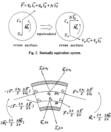
Let the force and torque on the cross section of the shaft be ~ and ~t~ with

-F = Vx~ + V,-?2 + NT3 (3)

where Vx, Vy are shearing forces, and N is the tension.

If the shearing forces V~TI + VrT2 do not act through the shear center Ss, it can be replaced by a statically equivalent system shown in Fig. 2 [30]. We obtain

~ e = ~ + s, Cs

x

(v j , + vj2)

(4)

where Cs is the centroid.

Applying the Bernoulli-Eulerian theory yields

(5)

The shaft behavior of BTA deep hole drilling tool

F = V,t, +V~te + N ts

equivcLten

~ -

v~r,+ v~7

cross seet~,o~z cross sect{,on

Fig. 2. Statically equivalent system.

465 At6Sl qt6s 1

\

/

- {r

-

~

a

s! 1

/

- ~u~ -~ ~ ~'J ~. ~s A.6S

Fig. 3. The small element cut from the shaft.

where k and k' are the component of curvature of the strained central line, z is the twist of the shaft and C, is the torsional with

C, = GJ.

2.2. Effect of fluid flow

Consider a small element of the shaft, with length 6s s (see Fig. 3). The corresponding mass of the enclosed fluid is 6my. p f is the density of fluid. Then

6m s = P s A s b s s .

The rate of change of momentum Ls can be written as:

d-i I

(02~

02~

U2 02~ OU

c~ I'~

dt = P s A f f s J ; \ O t 2 + 2 U o - ~ s / + --~-s} +-~-~sL]

(6)

dLfd___t_

_{= p~A~s~}

( ~

_{+ U ~}

0 ) 2

_{~(s~, t).}

₍₇₎

The results agree with the papers by Blevins [20], Paiduossis and Issid [22], Yoshizawa,

et al. [23], Lundgren et al. [25]. 2.3. Small defection

A small elements cut from the shaft is shown in Fig. 3. Coordinate transformation yields:

02y_

02X-

~-~Y3

A-t, = - Elx, ~s2 t, + EIy~ -~s2 tZ + GJ . (8)

(6)

466 Jih-Hua Chin e t al.

Let (~o)s and (~o)s be the rates of change of the angular momentum about O, and O r respectively. If the shaft deflection is small, the following equation can be obtained:

, 633y_ .1 633X- 1 6330- (]~o)s = - l~s at-~astl + l r s ~t--~st2 + I~ ~ - t 3 where l~s, I~, I~ denote the principal centroidal moments of inertia and

I~ = psI,~,6s; l~s = pslrsgs; I~s = psl:s6S.

Let

then

Similarly,

and the tension is:

- - 6 3 3 y - - 633 X - - 632 0 ~ h~ = - I~ ~ - 7 ~ t , + I , ~ - ~ s t ~ + h~ ~i-~t~. 633y _ a3X -- 6320_

her

= - I ~ I ~.-'2~'7-_ t ' + l r y ~ - ~ t 2 + I , I

-b-gt3

o r e s I o t v s I (9) (10)

The force equation is:

where where

632y

q~ = - p~,4~ ~i ~ + p s , 4 j + q~

The moment equation is:

t3 ×~ +~'3 ×~ + - ~ -

s

As = - p~hg, + Aes

AI

= -

P$ hoy + Ael.

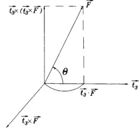
The following relations can be established from Fig. 4:

~'=NV~+T~x\ 63s

+ X , + X ~ .

dE s 63 2_

-~ = P I A s 6 s ( ~ t - U ~ s ) r(s,t).

63F 63P

63s

+ N +~; + ~ =°

(12)

(13)

(14)

2.4.

Equations of motion of BTA drill shaft with stationary cutting tool

In BTA drilling processes, the shaft is of uniform annular cross section, the points C,, C s, Ss are of the same location, and the points Os, O I become identical. So we can take:

l x s = I r s = I s ; I~ I = l y I = I I

and the flow velocity U is opposite to the direction defined earlier, so the rate of change of momentum

i f

of BTA drill becomes:

63w

(7)

?-

I

LL r

~3

Fig. 4. The relationship of the force in rectangular coordinates.

Substituting Eqn (14) into Eqn (12), the following general force equation can be obtained

+ x

(pd, + p/y) ~t-rAa~l t, +

(o,I, + o/y) ~tT~sJ t2

+-~S ( N - - P A f ) N - p s A s - ~ - p y A f + U-~s ~

+ (Ps As + pf Ay)g + -qe, + -qef dl- L aS 1'-73 X (~kes + ~kef)] = O. (15)

If we do not consider the twist z, the gravity ~, the external force, the external moment, the rate of the change of the momentum ~(p~l, o3x~ _{c~t2 ~M}_•""_'it is the same as the equation in Refs 1,,25] and 1,,26]. If we also neglect the kn, it is the same as the equation in Ref. 1,,20].

From i-'- in Eqn (15) the following form can be obtained by neglecting the high order terms

Os 2 8s2) Os ( P ' I ' + p y l Y ) ot2OsA+-~s

a2x

(a

a) 2

-- p, A~ ~ -- p y AS ~ -1- U-~s X - (Ps A, + pf Af)g

a 1' ~3 x ~es + mey)] = O. ( 1 6 )

If we do not consider the twist ~, the gravity-~, the external force, the external moment, the pressure P of the fluid flow, it is the same as the equation in Refs 1,,18] and 1,,19].

FromT3.in Eqn (15) the following equation is obtained

280s

(El~)k~ + EI= N ~ k,, +Ta'~s

(GJ z ~s x Os 2 ,]

~s 8U _ 827 .

+ (N -- PAy) -- pyAy - ~ -- (p~A. + pyAy)t3" 8t 2

+ (psAs + pfAf)~3"g+T3"(qes "[--qef)

-~---t3 "-'~S 1' t3 X (me, + "mef)] = 0 (17)

(8)

468 Jih-Hua Chin

et aL

(i z

]

;//A

k~

't

kT.

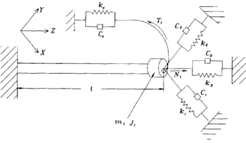
m z J, / /

Fig. 5. Boundary condition on the tool head.

If E, I,, U are constant and the twist z, gravity 0", external force, external moment are neglected, it is the same as the equation in Refs [25] and [26].

2.5.

Boundary conditions

The boundary conditions are constructed as that shown in Fig. 5. The condition at location s = l can be expressed by two models.

Model

1. The boundary condition contains the mass m~, the moment of inertia of mass J1, the forces, the torque, the springs and the dampers.

Model

2. The boundary condition at s = l is free while the mass m~, the moment of inertia of mass J~, the forces, the torque, the springs and the dampers are replaced by concentrated forces and torques.

3. THE SOLUTIONS OF EQUATIONS OF MOTION

The solutions of equations of motion of the BTA drill shaft will be given for the following general cases:

q-'~= = - c - ~ + f i (s,

t)i +f2 (s, t)j

+ f 3 (s, t)k" (18) - c ~ denotes viscous damping force and fl, f2, f3, are the external forces per unit where

length.

~'of = 0 (19)

- 80_

Ae= = - ct 8 t t2 +f4(s, t)k" (20)

where - c, ~ denotes viscous damping torque and f4 is the external torque per unit length.

A e f = 0. (21)

3.1. Lateral motion of the shaft

The equation of motion for lateral motion can be derived from Eqn (16):

~4X

84X

8 [

8X]

-- EI= ~ + (psi, + pflf) ~ + ~ (N - eAf) ~s

- - p=A=

-~-

- p f A f ~ t -4- ~,s X -- (Ps A s "k-

pfAf)g

8X

(9)

The shaft behavior of BTA deep hole drilling tool 469 B.C.'s ~X s = 0 , X = 0 , - ~ s - - 0 ~2X s = l , EIs--~s2 = 0 ~aX ~2X aX ~X s = l, EI~ -~-s3 = - m, - - ~ - - c t - ~ - k l X - N, -~s .

If m~, Cl in boundary condition are neglected it is similar to the equation in Ref. [ 2 2 ] . I.C.s t = 0 , X = g x l ( s )

dX

t = 0 , = xs(s).

Assume the solution of Eqn (22) is of following form:

X(s, t) = X~(s, t) + X2(s).

We first find Xs(s) by applying model 1 of the boundary conditions. Suppose

X2 = Xs~ + X2p

where Xzh is the homogeneous solution and X2j, is the particular solution. We have

s2(ps As + pfaf)g

X2p = - 2 ( _ N 1 + P t A f + p f A f U 2 ) "

Because N~ < 0 which is a compressive force we have

b~ = - Nt + P t A f + p f A f U 2

EI~

Xzh = d, sin bvs + d2 cos bvs - dlbvs - d2

where dl, d2 can be obtained from the following two linear equations:

~2X2(l) = - d~ b 2 sin bol - ds b~ cos bvl - (psAs + p f A f ) o = 0

as s -- Nt + P t A f + p t A f U s

- EI,( - dtb~ cosb~/+ dsbav sin b,,l) =

kl[dl(sin bvl - bd) + d2(cos b,,l - 1)

l 1

- 2( - Nt + P~A: + o : A : U2i - Nl dl(b~ cos b J ) - d2b~ sin b~l l(p~As + p : A / ) g ]

- _ p - ; - A s V 2 - j .

It is convenient to introduce the dimensionless quantities for X~:

X1 s

2,= T,

1 (.p Els_.. ~1/2

i = t-~ , A , + p f A y ) + p : l : _{U =}_UI_{( P f A f ~ 1/2} ip = 12(p~A ~ + p : A : ) ' \ E l , )

(10)

470 Jih-Hua Chin et al. p f a r p~A~ + p/A/)' m! fill = l(psA, + pfAf)' ~ = c 12 [EI~(psA~ + p/A/)] 1/2 I cl = c~ [El~(psA~ + p y - )j 12 Pt = PIAf l 3 12 13 gx3

0 3= T

Fix,, = gx41 (p,A, + p f A f ~ 1/2

_)'

and the equation is rearranged

as:

04 YG 04 X1 d g 4 lp Of 2 Og 2

0XI

- - + N t 6 ( g - 1) dg

02Xi

02.,~" 1 0 2 X I + 02 02X1 0X1 0221

+ e - y i - + m,a

1)

+ 5,6(g - 1) ~ + fq6(g - 1)S, = fl(g, F) (23) with B.C.'s

g=O, 21=0, --021=0

Og

0221

0321 O.

g=l, --~--=0,

Og----T=

The Galerkin method is used to find X1. Suppose that

M

)~,(g, i ~) = ~ ~b.,(g)q.,(t) ra=l

where q~.. (g) satisfy all the boundary conditions of the system. We take

~b,.(g) = cosh fling- cos fl,. g - a,.(sinh #,. g - sin fl,.g) where fl,. satisfies the equation

cos fl,. cosh fl,. + 1 = 0 and

(24)

(25)

(26)

sinh fl,. - sin fir. a,. cosh fl,. + cos fl,.

By the Galerkin method, the following equation in matrix form can be obtained: Aq + B(1 + Cq = f f f )

where A, B, C are M x M matrices and q, f, • are M x 1 matrices. We can write:

X , ( s , f) = (1)T(s)q(t)

(27)

(11)

where qff) is of the following form [31]:

q(~) = W=p e ~z J o e - ' s W ~ ~ A - t f ( z ) d z + W=p e ~J W -~ ~q~O)~, (29)

t" l x "~t

(4(0)

j

where J is the Jordan matrix, W = [W,~, W,o] T, W - ' = {-W~' W ~ ' ] , W = eigencolumn

matrix.

The matrices q(O), 4(0) are found by using I.C. and the orthogonality of ~b,(g) as follows: q,n(0) = ~ c~m(g)gxa(g)dg

4.(0) = f ' ~.(~)~,(~)d~.

d0 Finally, we obtain Xl(s, t) = Xl(,~, f ) l ---- ldpT(g)q(t) X(s, t) = X,(s, t) + X2(s).

This completes the solution of equations for lateral shaft motion. Y(s, t) can be obtained in a similar way by neglecting gravity.

3.2. Longitudinal motion of the shaft

The equation of motion for longitudinal motion can be derived from Eqn (17):

d2w d2w dw

EAs ~ - P d A : -- (psA~ + p : A:) - ~ - -- c ~ - +fs(s, t) = 0 (30)

Op 8~U w h e r e Pd ---- ~'~ = - - ~ [32]. B.C.'s: s = 0 , w = 0 dw t~2w aw s = l, EAs -~s = - ml -- ~ - - kaw - c3 --~ + N 1 I.C.'s t = 0 , w ( s , O ) = O l ( S ) t = 0, ~(s, 0) = 0z(S). Assume the solution of Eqn (30) is of following form:

wts, t) = w~(s, t) + w2(s).

We first find the static solution w2(s) by solving the following reduced equation:

t~2W2

EA~ ds 2 Pd A / = O.

It leads to

w 2 ( s ) = ~ - L s - ~ 2(EA~+k31) s 4 E A s + k a l S "

w,(s, t) is governed by the following reduced equation:

d2w, d2wl t~wl

EA~ ~ - (p~A~ + p: A:) - ~ - c - ~ - + f3(s, t) = 0

B.C.'s s = 1, EAs s = 0 , w, = 0 dwl ~2wl dw, ~s = --m~ ~ - - c 3 ~ - - k3Wl" (31)

(12)

472 Jih-Hua Chin et al. I.C.'s

t = O, w~(s, O) = g3(s) = gl(s) - w2(s) t = O, . q ( s , O) = g4(s) = e~(s).

It is convenient to introduce the following dimensionless quantities

b = ~ 1 1 + --psAs p~As b t ( EA, ~1/2 f = t ~ = -l \ p , A , + p / A / , ] l ( = C [EA~(p, As + p f A f ) ] 1/2

1

C3 = C3 [EA~(p~A, + pfA:)] t/2 l g3 (74 f a = f a ~-~,, O 3 = - f , g,, = --~ o~ = f~l (p,A~EA,

+ P/ A(~l/2J

and the equation is normalized as

~2W 1 ~2W 1 02W1 ~21~ 1

- a - - T + ~ + e ~ +

,~, -~- a(~

- 1) - ~ w l ~ . -

+

ca'--~-ots - 1) + k3#~a(g - 1) =fa(s, f) with B.C.s

g = 0 , ~ 1 = 0 g = 1, - 0 .

Again the Galerkin method is used to find Wl. Suppose that

M

~1(~, t-) = ~, Ckm(g)qmff) m = |

where ~bm(g) satisfy all the boundary condition of the system. We take

~bm(g) = sin 2m s, where 2~ = (2m - 1)n ₂ _{, m = 1 , 2 ....} The ~m(s) are orthogonal over the span of the cantilever.

By following operation similar to that in Section 3.1, we can obtain Aij + Bd 1 + Cq = f ( f )

where A, B, C are M x M matrices and q,f, • are m x I matrices. Using

q,(0) =--m,,l[f~¢,(~)g3(g)dg

1

dq,(O)d_t = mi--~-l[f2 O,(g)g,(g)dg]

(32)

(33)

(13)

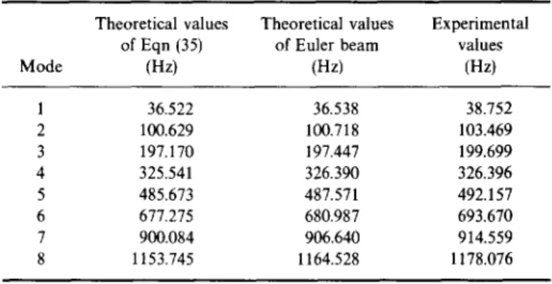
Table 1. The natural frequencies of lateral vibration of the shaft of BTA drill (hanged horizontally with no fluid)

Mode

Theoretical values Theoretical values Experimental of Eqn (35) of Euler beam values

(Hz) (Hz) (Hz) 1 36.522 36.538 38.752 2 100.629 100.718 103.469 3 197.170 197.447 199.699 4 325.541 326.390 326.396 5 485.673 487.571 492.157 6 677.275 680.987 693.670 7 900.084 906.640 914.559 8 1153.745 1164.528 1178.076

where mii = ½, the q(t-) can be found by the same method is Section 3.1. Finally, we obtain

w,(s, t) = g'l(g, f)l = lq~(g)q(f)

w(s, t) = ~l(s, t) + w~(s).

This completes the solution of equations for longitudinal shaft motion.

4. SYSTEM SIMPLIFICATION

The foregoing equations of motion were established in a general sense. They could be simplified to cope with the practical engineering features.

F o r example, the tool shaft is of steel material so that the deformation is small and the effect of rotatory inertia could be neglected. This leads to an Euler Beam. In order to m a k e system simplification the following two preliminary system analyses are performed.

4.1. System eigenproperties--solid shaft

The equation of motion in lateral direction can be derived from Eqn (22) as follows:

~*X ~2X ~X c~*X

EI, ~ + psAs ~ + C ~ - psi, 0s--5~ = 0. (35)

This equation can be further simplified to become an Euler beam equation:

?,*X ~2X ~X

EI, ~ + p, As ~ + C ~ - = 0. (36)

The following b o u n d a r y conditions are used to investigate the shaft eigenproperties. d2X ~3X

s---0, ~-~-32 - (~$3 - 0

?,2X daX = 0 .

The natural frequencies of modes 1-8 of the two theories and of experiment are listed in Table 1 which reveals that theoretical values of Euler Beam are closer to the experimental values than those predicted by Eqn (35).

4.2. System eigenproperties--solid shaft with static fluid

The purpose of this analysis is to examine the system under the influence of the static fluid.

The equation of motion can be rewritten from Eqn (22) for lateral shaft motion as follows:

~4X c~2X ~X ~4X

(14)

474 Jih-Hua Chin

et al.

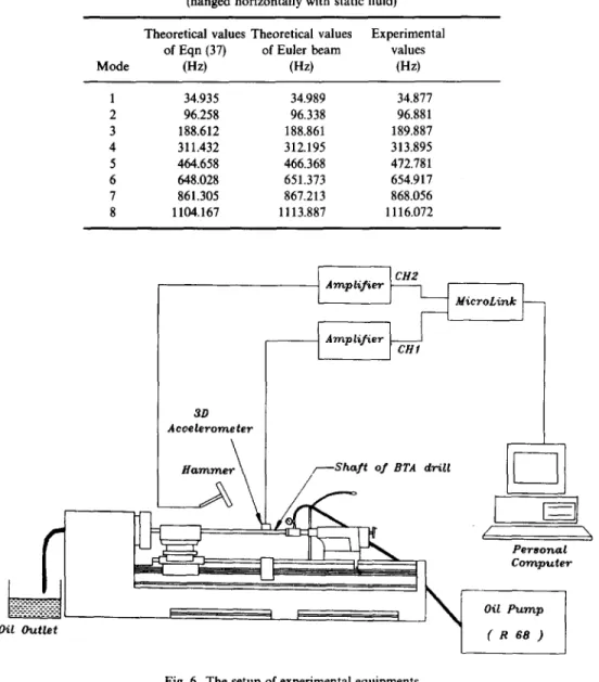
Table 2. The natural frequencies of lateral vibration of the shaft of BTA drill (hanged horizontally with static fluid)

Mode

Theoretical values Theoretical values Experimental of Eqn (37) of Euler beam values

(Hz) (Hz) (Hz) 1 34.935 34.989 34.877 2 96.258 96.338 96.881 3 188.612 188.861 189.887 4 311.432 312.195 313.895 5 464.658 466.368 472.781 6 648.028 651.373 654.917 7 861.305 867.213 868.056 8 1104.167 1113.887 1116.072

t Amplifier ~ 1

~

Amplifier]CHf

MieroL irtk

Oil

Outlet 39

Acvelerometer

tlammer\

/~Shaft of BTA drill

- / PeTso'n~.[

Compufer

Oil Pump

( R 6 8 )

\

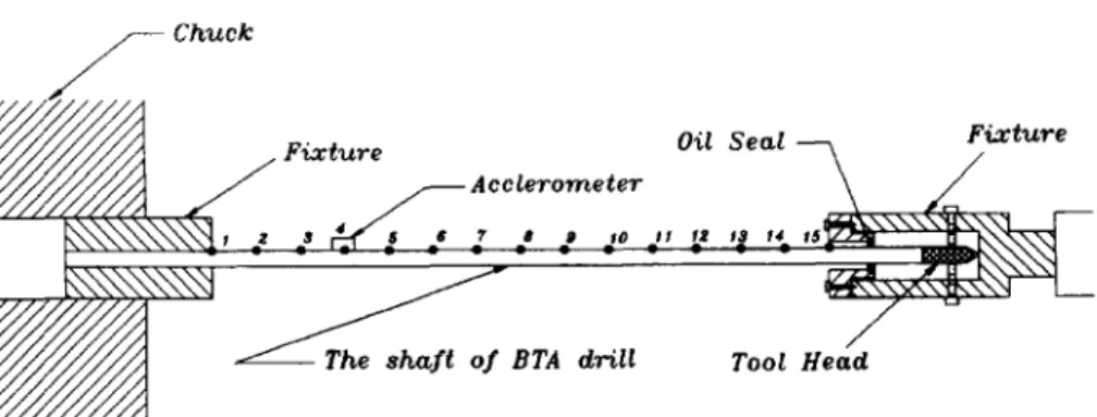
Fig. 6. The setup of experimental equipments.

The equation of motion of an Euler Beam is:

b4X ~ZX 8X

El, ~ + (psA~ + p/A:) - ~ - + C ~ = 0. (38) Both system equations are subjected to the same boundary conditions as that in Section 4.1.

Comparing the theoretical values of natural frequencies of modes 1-8 with those of experiment in Table 2, it is seen again that the theoretical values of an Euler Beam are closer to the experimental values than those predicted by Eqn (37).

Based on the results of the above two series of preliminary analyses, the proposed equations of motion can be simplified and the shaft of the BTA drill be taken as an Euler Beam. In the following studies only the simplified equations of motion will be used.

5. T H E E X P E R I M E N T A L A R R A N G E M E N T S

The experimental arrangements are shown in Fig. 6, in which a heavy duty lathe is equipped with self-designed fixtures to hold the drill on both ends. The experiments which involve generally modal testing techniques 1-33, 34] are divided into two parts:

(15)

The shaft behavior of BTA deep hole drilling tool

Chuel¢

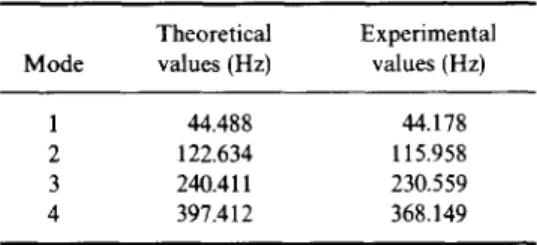
Fig. 7. The arrangements of experiment (shaft without fluid, both ends are clamped).

475

(1) The shaft of the BTA drill is installed on the machine without introduction of oil. (2) The shaft of the BTA drill is installed on the machine with both ends fixed and oil is

supplied.

Details of the experimental arrangements are as follows:

1. Lathe:

SAN S H I N G SK26120 HEAVY DUTY P R E C I S I O N LATHE. (Distance between chuck center and tailstock center: 3m) 2. Hammer:

Hammer: PCB 086B05 SN5163 (range: 0-5000 lb) Amplifier: PCB model 4801906 power unit. 3. Accelerometer:

accelerometer: TEAC 601Z (weight: 0.3 g) amplifier: TEAC SA620.

4. Data acquisition system:

MicroLink: four independent channels, stand-alone type with 64k samples per channel on-board memories. 5. The deep hole drill:

a. drill head:

Type: SANDVIK 420.6-0014D 18.91 70 Mass: 0.030205 kg

Mass moment of inertia J~: 1.420 x 10- 6 kg. m 2. b. drill tube: Type: S A N D V I K 420.5-800-2 Length: 1.6 m Internal diameter: 11.5 mm External diameter: 17.0 mm Material: JIS S N C M 21 Density p,: 7860 kg/m 3 Young's modulus E: 2.06 x 1011 Pa Shear modulus G: 8.1 x 10 l° Pa 6. Fluid: Type: R68 Density Ps: 866 kg/m 3 Absolute viscosity #: 0.383 kg/m. s. 6. T H E S H A F T B E H A V I O R I N I N S T A L L E D C I R C U M S T A N C E S

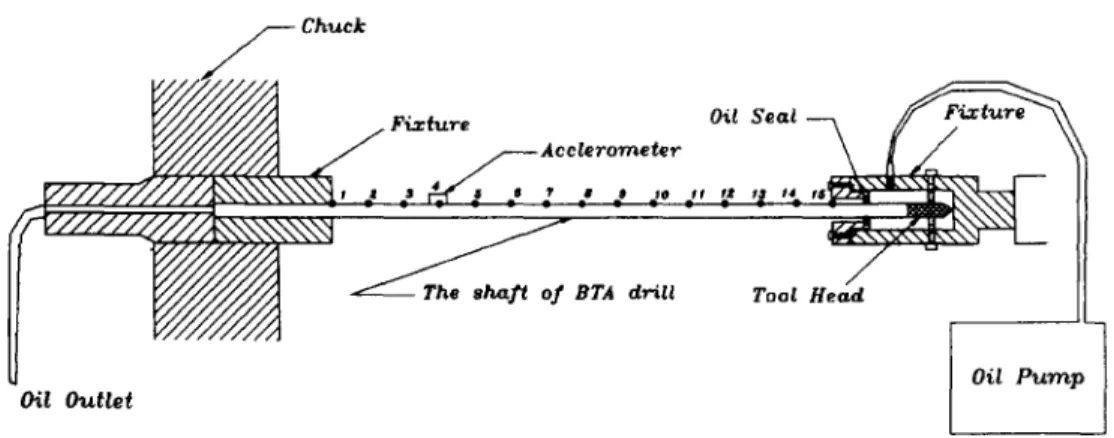
The shaft is installed on the lathe by the fixtures and the shaft behavior in installed circumstances is investigated in this section. The arrangements of this experiment are shown in Fig. 7.

The equation of lateral motion is"

O*X 0 2 X OX EIs ~ + Ps As - ~ - + C ~ = 0 (39) with B.C.'s dX s = 0 , X - - 0 Os ~ 2 X 03X s = l, t3s2 - ~ = 0. MS 3E:5-B

(16)

476 Jih-Hua Chin et al.

Table 3. The natural frequencies of lateral vibration of the shaft of BTA drill (both ends clamped horizon-

tally with no fluid)

Mode Theoretical Experimental values (Hz) values (Hz) 1 44.488 44.178 2 122.634 115.958 3 240.411 230.559 4 397.412 368.149 Let X(s, t) = X~b(s) q(t).

The mode shape function q~j(s) can be obtained from the boundary conditions: ~bj(s) - cosh fijs - cos flis - ~j(sinh fljs - sin fljs)

and

(40)

The theoretical natural frequency is equal to

1 . ~ _ ~ EI~

f" = ~ ~/ psA-~ " (42)

The frequency response function is

M

14(s,, s , w) = y~ 4~/s,) 4~j(s,) haw).

j = l

a. Natural frequency

In this experiment, the tool head is fixed with two bolts and an oil seal ring is present which makes the practical boundary condition complex and not ideal. The comparisons between the theoretical and the experimental values of natural frequencies of modes 1-4 are listed in Table 3 in which the agreement can be seen, but the discrepancies are somewhat larger than that in Tables 1 and 2.

b. M o d e shape

The mode shape function of the shaft is

q~j(s) = cosh fi~s - cos fljs cosh fir - cos fir

- sinh fljl sin fir (sinh fljs - sin fljs). cosh fir - cos fl)l

~tj = sinh fir -- sin fir cosh f i r . c o s fir = O. Giving an impulse to the shaft yields

~4X ~2X ~ X

El~-~s4 + P s A ~ - - ~ + C ~ - [ = h(t).

By doing the Fourier Transform of the above equation and solving for the closed form, the solution yields

(17)

The shaft behavior of BTA deep hole drilling tool 477 Normalized

displacement

1 0.8

f

0.6 0.4 0.2 0 -0.2 -0.4 - 0 . 6 - 0 . 8 -1 D

o.2 o.4 o.e o.a 1 1.2 1.4

Length of the shaft (m)

1,6

- - T h e o r y - - a -

Experiment

Fig. 8. The shape of mode 1 for lateral vibration (shaft without fluid, fixed-fixed).

Normsllzed

displacement

1 0.8 0.6 0.4 0.2 0 E - 0 . 2 - 0 . 4 - 0 . 6 - 0 . 8 - 1 0 [3 O 0.2 0.4 0.6 0.8 1 1.2 1.4

1.6

- - T h e o r y ~

Experiment

Fig. 9. The shape of mode 2 for lateral vibration (shaft without fluid, fixed-fixed).

Normalized

displacement

1 o 0.8 0.8 0.4 0.2 O= - 0 . 2 - 0 . 4

-0.6

- 0 . 8 ., I I I ; I ~ I O 0.2 0.4 0.6 0.8 1 1.2 1.4 1.6

- - T h e o r y ~

Experiment

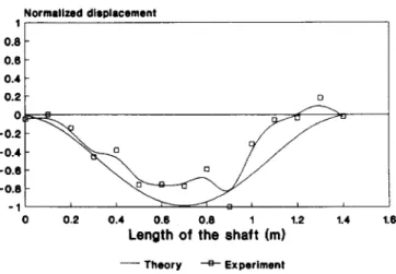
Fig. 10. The shape of mode 3 for lateral vibration (shaft with fluid flow, fixed-fixed).

The mode shape of modes 1-3 according to the above equation are compared with the experimental result in Figs 8-10. We find all the theoretical mode shapes are in agreement with the experimental counterparts.

Although some discrepancies due to the practical clamping and sealing are seen, the experiments conducted in this section have confirmed the general agreement between the

(18)

478 Jih-Hua Chin et al.

~

Chuck j Fixture//~-~-AeelerOITteter ~ / / / / / ~ . \ \ \ \ \ \ \ \ ? , 7 - t / / / / / / / / / / / / A , , ~ , q fill Outlet Oil S~a~ - ~

~

BTA

drill

Toot

Hea(

Oil Pump

Fig. 11. The arrangements of experiment (shaft conveying fluid).

practical fixture effects and the ideal boundary conditions. This is very encouraging for future research since mathematical tools are obtained for this conventionally empirical area.

7. THE SHAFT BEHAVIOR OF THE BTA D R I L L WITH C U T T I N G F L U I D

In this section, the behavior of the shaft conveying fluid is investigated. The arrangements of this experiment are shown in Fig. 11.

The fluid pressure on the tool head Pt is read from a pressure gauge to be:

Pt = 3.92 x 106 N / m 2.

Due to the limit of the available hydraulic system the flow rate cannot be changed. We have

Flow rate = 1.2 x 10 -4 ma/s Flow velocity = 1.155 m/s. The equation of motion is:

d4X _dX 02X EI~ (N - PAy) - U ~ X + C = 0 (43) with B.C.'s OX s = 0 , X - - 0 Os OX s = l , X = - - = 0 . Os

In this experiment, the axial force N is zero. Rearranging the above equation yields

(~4X ~2X (~2X O2X C t~X

E l , - ~ s , + ( P t A I + pyAIU2)-~s2 - 2 p f A f U ~ s & + ( p , A , + pyAy)-~-fi-s2 + - ~ - = 0 . (44) Let

X(s, t) = X dp(s)q(t)

the mode shape function ~bj(s) is

(19)

The shaft behavior of BTA deep hole drilling tool 479 Table 4. The natural frequencies of lateral vibration

of the shaft of BTA drill (both ends clamped horizontally, conveying fluid)

Theoretical Experimental Mode values(Hz) values(Hz)

1 43.424 43.015

2 119.689 112.382

3 234.634 220.889

and

cosh fl jl - cos tiff

% - sinh fljl - sin tiff

cosh fljl. cos tiff = 1.

Giving an impulse to the shaft, the equation of motion becomes

c~4X c~2X c~2X t32X c~X

EIs ~S-dS , + (Pt AI + Ps As U2) ~ - 2Ps Af U ~sOt + ( P2 As + Ps As) ~ - + C --~ = h(t). By doing the Fourier Transform of the above equation and solving for the closed form solution, we can obtain

Hi(w) = 1 1 w 2 p A U2) O2A'' EI~fl~(o + (PtAr + y y vs w (psA~ + pfAy)(o ) - i ( - E l s f l ~ P + ( P J A ? + p f A f U 2 ) f l 2 $ " ) " \cTc~---2--pfA - ~

The theoretical natural frequency is equal to

X/

g2) R%"

1 EIs l~jq~ + (PrAy + py Af ,'J f" = ~ (p,A, + pyAf)c~ The frequency response function is

a. (46) (47) M H(s~, s,, w) = ~ ckj(s~) (pj(s,) H~(w). j = l Natural frequency

Comparing the theoretical values of natural frequencies of modes 1-3 with those of experiment in Table 4, we can find the theoretical values of natural frequencies being close to the experimental values.

b. Mode shape

The mode shape function of the shaft is

4aj(s) = coshfljs - cosfljs cosh fljl - cos fljl

- sinh fljl sin tiff (sinh f l j s - fljs).

The theoretical and experimental mode shapes are compared in Figs 12-14. It is seen that the agreements are satisfactory, but the fluid has caused even larger discrepencies.

(20)

480 Jih-Hua Chin et al. Normalized displacement 0.8 0.6 0.4 0.2 0 -0.2 -0.4 -0.6 -0.8 I I I I I I I 0 0.2 0.4 0.6 0.8 1 1.2 1.4 1.6

- - Theory ~ Experiment

Normalized displacement 1 0.8 0.6 0.4 0.2 0 ~ - 0 , 2 - 0 . 4 -0.6 -0.8 - 1 0 I I I 0.2 0.4 0.6 1.6 Length o f t h e s h a f t ( m ) 0.8 1 1.2 1.4 - - T h e o r y ~ E x p e r l m e n t

Fig. 13. The shape of mode 2 for lateral vibration (shaft with fluid flow, fixed fixed).

Normalized displacement 1 o 0.8 0.6 0.4 0.2 0 - 0 . 2 - 0 . 4 - 0 . 6 - 0 . 8 I -1 t I I l I I I 0 0.2 0.4 o.s o.e J t.2 1.4

1.6

- - Theory --R- Experiment

8. C O N C L U S I O N

The shaft behavior of deep hole drilling is important in the cutting process but rarely studied. This paper studied the tool shaft of deep hole drilling by treating the shaft as a pipe and using the Bernoulli-Eulerian theory. The general equations of motion for the BTA drill shaft are rigorously derived which can be reduced to different specific equations of former

(21)

works. The constructed general equations govern the lateral, longitudinal and torsional motion of a tool shaft conveying pressurized fluid.

The solutions for lateral and longitudinal motion are obtained by combined analytical and Galerkin methods.

A preliminary comparison between theoretical and experimental results shows that the

I ~4x

rotatory inertia effect is negligible and the term p ex2~ in the shaft dynamics can be deleted. The shaft can be treated as an Euler Beam.

Two series of experiments are performed to verify the lateral shaft dynamics for an installed tool with and without cutting fluid. Although the boundary conditions of fixture damping are not ideal, the comparisons of natural frequencies and shaft mode shapes between theoretical and experimental results are satisfactory. Since the natural frequencies are lower than those of usual cutting tools, and the rotating workpiece might worsen these values, it can be predicted that the shaft dynamics are not negligible in the cutting process. The constructed general equations of motion for a tool shaft build a foundation of knowledge about it and pave the way for future studies concerning correlation between cutting process and shaft behavior.

Acknowledgement The authors thank the National Science Council of the Republic of China for the support of this study under the Grant Number NSC-81-0401-E4)09-13.

R E F E R E N C E S

1. E. Flegel, Deephole drilling machine and tools for economic drilling operations. Industrial Prod. Engng 9, pp. s22, s24, s26, s28 (1985).

2. P. Rudd and 1. Hetherington, Advances in precision holemaking. Manuf Engng 102, 87-89 (1989). 3. P. K. R. Rag and M. S. Shunmugam, Accuracy and surface finish in BTA drilling. Int. J. Prod. Res. 25, 31-44

(1987).

4. P. K..R. Rag and M. S. Shunmugam, Investigation: stress in boring trepanning association machining. Wear 119, 89-100 (1987).

5. P. K. R. Rag and M. S. Shunmugam, Analysis of axial and transverse profiles of holes obtained in B.T.A. machining, lnt. J. Machine Tools Manuf 27, 505-515 (1987).

6. P. K. R. Rag and M. S. Shunmugam, Wear studies in boring trepanning association drilling. Wear 124, 33 43 (1988).

7. M. M. EI-Khabeery, M. M. Saleh and M. R. Ramadan, Some observations of surface integrity of deep drilling holes. Wear 142, 331-349 (1991).

8. J. Corney and B. Griffiths, A study of the cutting and burnishing operation during deep hole drilling and its relationship to drill wear. Int. J. Prod. Res. 14, 1-9 (1976).

9. K. Sakuma, K. Taguchi and A. Katsuki, Study on deep-hole-drilling with solid-boring tool the burnishing action of guide pads--and their influence on hole accuracies. Bull. J S M E 23, 1921-1928 (1980).

10. K. Sakuma, K. Taguchi and A. Katsuki, Study on deep-hole boring by BTA system solid boring tool--behavior of tool and its effect on profile of machined hole. Bull. Japan Soc. Precision Engng 14, 143 148 (1980).

11. A. Katsuki et al. The influence of tool geometry on axial hole deviation in deep drilling: comparison of single- and multi-edge tools. J S M E 30, 1167-1174 (1987).

12. M. G. Yumshtyk and S. S. Kedrov, Gun drill vibration in deep drilling. Machines & Tooling 39, 34-36 (1968). 13. K. Sakuma, K. Taguchi and A. Katsuki, Self-guiding action of deep-hole-drilling tools. Ann. CIRP 30, 311 315

(1981).

14. Catalog, Drilling Tools, HV-1200:2-ENG, SANDVIK Coromant (1983).

15. J. H. Chin, J. S. Wu and R. S. Young, The computer simulation and experimental analysis of chip monitoring for deep hole drilling. ASME, J. Engng Indust. 115, 184-192 (1993).

16. J. H. Chin and J. S. Wu, Mathematical models and experiments for chip signals of single-edge deep hole drilling. Int. J. Machine Tools Manuf 33, 507 519 (1993).

17. J. H. Chin and S. A. Lin, Dynamic modelling and analysis of deep hole drilling process, Proc. Pacific-Rim Int. Conf. Modelling, Simulation and Identification, IASTED, Vancouver, pp. 131 134 (1992).

18. S. Chandrashekhar, T. S. Sankar and M. O. M. Osman, A stochastic characterization of the machine tool workpiece system in BTA deep hole m a c h i n i n ~ P a r t I. Mathematical modelling and analysis. Adv. Manuf Processes 2, 37-69 (1987).

19. S. Chandrashekhar, T. S. Sankar and M. O. M. Osman, A stochastic characterization of the machine tool workpiece system in BTA deep hole m a c h i n i n ~ P a r t II. Response analysis and evaluation of the tool tip motion. Adv. Mant~ Processes, Vol. 2, 71 104 (1987).

20. R. D. Blevins, Flow-Induced Vibration, Chapter 10. Krieger Publ. (1986).

21. M. P. Paidoussis, Dynamics of Tubular cantilevers conveying fluid. J. Mech. Engng Sci. 12, 85 103 (1970). 22. M. P. Paidoussis and N. T. Issid, Dynamic stability of pipes conveying fluid. J. Sound Vibr. 33, 267 294 (1974).

(22)

482 Jih-Hua Chin et al.

23. M. Yoshizawa et al. Buckling and postbuckling behavior of a flexible pipe conveying fluid. Bull. J S M E 28, 1218-1225 (1985).

24. J. M. T. Thompson and T. S. Lunn, Static elastic formulations of a pipe conveying fluid. J. Sound Vibr. 77, 127-132 (1981).

25. T. S. Lundgren, P. R. Sethna and A. K. Bajaj, Stability boundaries for flow induced motions of tubes with an inclined terminal nozzle. J. Sound Vibr. 64, 553-571 (1979).

26. W. S. Edelstein, S. S. Chen and J. A. Jendrzejczyk, A finite element computation of the flow-induced oscillations in a cantilevered tube. J. Sound Vibr. 11)7, 121-129 (1986).

27. J. L. Hill and C. P. Swanson, Effects of lumped masses on the stability of fluid conveying tubes. A S M E J. Appl. Mech. 494-497. June (1970).

28. Y. Sugiyama et al. Effect of a spring support on the stability of pipes conveying fluid. J. Sound Vibr. 100, 257-270 (1985).

29. A.E.H. Love, A Treatise on the Mathematical Theory of Elasticity, 4th Ed. Chapter XVIII. New York (1994). 30. J. M. Gere and S. P. Timoshenko, Mechanics of Materials, 2nd Ed. Wadsworth (1984).

31. D. E. Newland, Mechanical Vibration Analysis and Computation. John Wiley (1989). 32. R. W. Fox and A. T. McDonald, Introduction to Fluid Mechanics, 3rd Ed. John Wiley (1989). 33. D. J. Ewin, Modal Testing: Theory and Practice. Research Studies Press (1986).

34. H. Goldstein, Classical Mechanics, 2nd ed. The Southeast Book Co. (1989). 35. E. A. Brandes, Metal Reference Book, 6th Ed. Butterworths (1983).

36. W. F. Chen and T. Atsuta, Theory of Beam-Columns, Vol. 2. Space Behavior and Design, Chapter 2. McGraw-Hill (1977).

37. J.H. Chin and L. W. Lee, A study on the tool eigenproperties of BTA deep hole drill theory and experiments. Accepted by Int. J. Machine Tools Manuf. (1994).

38. D. J. Gorman, Free Vibration Analysis of Beams and Shafts. John Wiley (1975). 39. Japanese Standards Association, JIS 1987-1988 Ferrous Materials and Metallurgy. 40. R. B. Ross, Metallic Materials Specification Handbook, 4th Ed. Chapman & Hall (1992).

41. R. H. Sabersky, A. J. Acosta and E. G. Hauptmann, Fluid Flow a First Course in Fluid Mechanics, 3rd Ed. Macmillan (1989).

42. W. T. Thomson, Theory of Vibration with Applications, 3rd Ed. Prentice-Hall (1988).

43. F.S. Tse, I. E. Morse and R. T. Hinkle, Mechanical Vibrations Theory and Applications, 2nd Ed. The Southeast Book Co. (1979).