Pergamon
Computers & Geosciences Vol. 22, No. 9, pp. 1033-1049, 1996 Copyright IQ 1996 Elsevier Science Ltd PII: SOO98-3004(96)00042-8 Printed in Great 0098-3004/96 St500 + 0.00 Britain. All rights reserved
A XERION-BASED PERL PROGRAM TO TRAIN A NEURAL
NETWORK FOR GRID PATTERN RECOGNITION
JEHNG-JUNG KAO
Institute of Environmental Engineering, National Chiao Tung University, Hsinchu, Taiwan 30039, R.O.C.
e-mail: [email protected]
(Received 27 April 1995; revised 5 December 1995)
Abstract-Neural network training with the back propagation algorithm is an important artificial intelligence technique for grid pattern recognition. The training is time-consuming however and generally requires a trial-and-error procedure to configure the network. A Per1 program executed with Xerion is presented to relieve the training burden. Statistical reports such as computation time, learning performance, and validation performance are generated automatically by the program. A case study applying the program for training networks to determine a drainage pattern from Digital Elevation Model data is demonstrated and discussed. Manually determining drainage patterns from topographical maps for a grid-based model is tedious and subjective. The neural network has a self-learning capability that can replace human judgment involved in the conventional approach. Copyright 0 1996 Elsevier Science Ltd
Key Words: Neural network, Grid pattern, Digital Elevation Model, Drainage pattern.
INTRODUCTION
Human judgment to determine a grid pattern for a geographical feature from a topographical map, image, or aerial photograph, involves not only the attributes of a grid cell but also the spatial distribution of adjacent grid cells. Such a manual approach is time-consuming and generally subjective. A program in a conventional language (e.g. C or FORTRAN) or an expert system is used typically to replace such a manual determination. The spatial distribution and relationships among grid attributes, however, introduce complexity for a program or expert system to consider numerous variants of grid patterns. Such complexity may make the program or expert system inefficient compared to the conven- tional manual method. A neural network method thus is explored for its potential applicability.
Several difficulties may occur during implemen- tation, even though the neural network method is now studied widely. Training a network to learn from a set of training data may require extensive computation before convergence to an optimum. Local optima instead of the global optimum may occur in determining a set of weights for network links during training. Another major difficulty is that no theory is available yet to construct an appropriate network configuration for a general problem, even though the optimum number of hidden nodes in the training cycle have been determined in previous research (e.g., Mirchandani and Cao, 1989). The optimal configuration of a neural network is still an important research issue. A trial-and-error procedure is employed generally by applying various learning
methods and testing several different configurations. Such a process is however time-consuming and tedious. Preparation of training reports from numerous results obtained by applying different network training strategies and configurations are also cumbersome.
This paper presents a program written in Per1 (Wall and Schwartz, 1992) to apply Xerion (Camp, Plate, and Hinton, 1993), a neural network package, for training neural networks with various methods and network configurations in a batch fashion. The user can leave the program as a background job and results are summarized automatically. Intermediate training progress is reported to the user through an electronic mailer. It is believed that a neural network study can be implemented effectively with the program. A case study applying the program to train and to find a neural network for determining a drainage pattern from Digital Elevation Model (DEM) data is demonstrated.
OVERVIEW OF BACK PROPAGATION NEURAL NETWORKS AND XERION
An artificial neural network is made up a number of layers of highly interconnected simple processors. A neural network generally is trained with a set of training patterns of which both input stimuli and corresponding output response are known. Once the network is trained completely, it is then applied as a transfer function to provide desired output patterns from given untrained external inputs. The advantages of a neural network include generalization, massive 1033
parallel processing, self-organization, etc. A good network trained from a proper set of training cases is capable of giving the appropriate response to a given input pattern, even if a certain degree of noise exists within the input pattern. A well-trained network can make generalizations from learned training patterns similar to an unfamiliar input pattern to produce a desired output response without user intervention or supervision. These advantages make it attractive to build a neural network for grid pattern recognition.
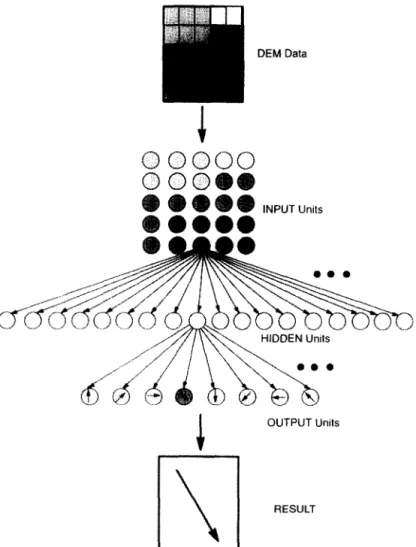
In this study, the popular three-layer network, as shown in Figure 1, with input, hidden, and output layers is used. Nodes are interconnected with numerous links whose strengths are expressed by numerical values named weights. Each node is activated from a function of the sum of the inputs received from other nodes through the weighted links. For a neural network to learn a set of training patterns involves modifying the weights via a learning algorithm. The back propagation approach applied frequently for this learning purpose was used in this study.
As this approach is described in detail by Rumelhart and others (1989), only a brief description follows. The implementation includes two stages. In the first stage, the output vectors obtained from a neural network according to the input vectors of a given training set are determined based on an initial weight set. Comparison of output vectors with the desired output (“target”) vectors is made at the end of the first stage. A back propagation learning procedure, the second stage, is then initiated if differences (or “errors”) result from the comparison. The differences are used as error signals to propagate backward through the network to correct the weights. This two-stage procedure is repeated until all the given training patterns are learned correctly.
The following summed square function is used to measure the error:
E =
CEp
=
C&p,
- op.)’
P P I\ 1
where p ranges over all input patterns, i ranges over output nodes, E,, is the error on pattern p, r,, is the
DEM Data
INPUT Units
OUTPUT Units
RESULT
A neural network for grid pattern recognition 1035
target value of a node, and Opi is the output (activation) value of a node. A direct method such as steepest descent then can be applied to find the set of weights that minimizes this function. For example, the weight on each link (between nodes i and j) can be modified on the basis of the error signal and the output value, A, y, = $,o,, where 6 is the step size factor, p is the input pattern number, and 6 is the error. For an output node, 6 is computed with S,, = (r,, - o,,)J(ner,,), wherex(ner,,) is the derivative of an activation function, such as the logistic equation shown subsequently in this section. For a hidden node, however, there is no desired target, and the error signal is determined from hp, =_f~(net,,)Z&,~~~,, where 6, are the error signals of the nodes to which the hidden node directly connects and M’~, are the weights of the connections. This procedure is based on the method of steepest descent with a fixed step size. This method, however, may not perform well and other algorithms for nonlinear optimization such as the conjugate gradient method are applicable also.
Xerion is a publicly accessible neural network package developed by Camp, Plate, and Hinton (1993). A collection of C libraries is provided to implement many neural network paradigms. Besides the back propagation network, the package provides also the Boltzmann machine, the mean-field-theory machine, hard and soft competitive learning, the Kohonen, cascade correlation, and recurrent back propagation networks. The user interface, which is built on X-windows, provides a friendly environment for either a novice or an experienced user to implement interactive training. The bp module of the Xerion (Camp, Plate, and Hinton, 1993) system implements the back propagation learning algorithm. Other than the steepest-descent method, the package also provides the methods of momentum descent, conjugate gradient, Rudi’s conjugate gradient, and others, described by Camp, Plate, and Hinton (1993); only a brief description follows.
Momentum-descent method
This method sets the direction to be the steepest descent with a momentum term. The momentum term is the previous direction multiplied by a decay factor, u, as shown in Equation (2).
Aw,j(n + 1) = q(6,0,,) + aAw,(n). (2)
This method is intended to decrease the amount of wandering in ravines of the error surface.
Conjugate-gradient method
This method, based on the method described by Press and others (1992), is expressed according to Equation (3):
s “**
= s
(G,,. - Wk.
_
GG.G “0”’ 3 (3)
where S.,, is the new search direction, S is the previous search direction, G,,.. is the current gradient, and G is the previous gradient.
Rudi’s conjugate-gradient method
This method modified by Rudi Mathon (Camp, Plate, and Hinton, 1993) from the previous method is expected to provide rapid convergence. The search direction is expressed as:
S.G.,,,
” =
(Gn,,,
- ‘XG,,,, - G)
(Cm - GWn,.
2SG>,
‘* =
(G,,..-
G).(G.,,,-
G)-
(G.,,.-
G)SSm,, = u,*(G.,, - Cl + u,*S - u,*G,,,,
Step methods
(4)
Once the search direction is determined, the step size should then be determined. Two types of step methods were provided by Xerion: a fixed step and a line search. The former uses a fixed size of step. A line search method is intended to find the minimum value of a function along a given search direction. For example, if W is the current weight set (starting position) and S is the search direction vector, the line search should find q that minimizes the error function E(W+ f) S).
THE PERL SCRIPT PROGRAM
Per1 (Wall and Schwartz, 1992) is a freely available script language to manipulate text, files, and computational processes that were implemented previously with complex programming in C, AWK (Aho, Kerninghan, and Weinberger, 1988) or a shell script language. The script program is written in Per1 to operate with Xerion in a batch fashion. Although the interactive display provided with Xerion is useful for learning and monitoring training strategies, it is tedious to manipulate inputs and reports for massive training strategies using various learning methods, network configurations, and numbers of nodes in each layer. The pseudocode listed in Table 1 describes the execution flow of the script program listed in the Appendices. The user must provide a file including all training cases and a validation file including all testing cases to verify the results obtained from a trained network. Two other files must be provided also by the user to specify formats for reporting the result and validation outputs, shown in Appendices 2 and 3. The script program frequently is executed as a background job on a UNIX workstation. A typical command to run the script is listed next, although other commands such as crontab can be used also.
nohup per1 doNet demRnet dem.train dem.velid > & /dev/null &where doNet is the
Table I. Pseudocode of Per1 script program, doNet
Usage: doNet netName trainingFileName validationFileName [#_ofinput-nodes #_of_output_nodes] main program:
Set user-defined variables (or use default values): #_of_hiddeuodes, email address, etc. Initialization for this run, netsame:
create a directory named by netName for keeping information for this run. link files (use ‘In’ instead of ‘cp’ to save space).
Disable the Xerion X-window display.
If the user provides a user specified reporting file, ‘report. sub, include it into the script program. for each specified #_ofL_bidden_nodes do
(
l.set learning method and related parameters.
2.call function doNet to implement a training and validation path. 3. repeat 1. and 2. until all desired learning strategies are implemented. )
Function doNet:
Set a unique identification for current training and validation path. Set input and output file names.
Create a tag for monitoring the training progress.
If the user’s email address is provided, the tag is sent to the user. Implement the training stage:
Write Xerion bp input command files by calling function writeNetIn. Implement the training by Xerion bp module in batch mode.
Computation time is logged to a time report file. Implement the validation stage:
Write Xerion bp input command files by calling function WriteNetIn.
Implement the validation stage by Xerion bp module in batch mode with weights obtained in the training stage. Computation time is also logged to a time report file.
Implement the user specified reporting function (reportsub) to generate statistical summary report. Function reportsub:
General steps:
Extract computation time summary from the time report file created by doNet. Extract the first iteration and last iteration information from Xerion bp output. Problem dependent steps for the case study: (implemented by function compare) Report the summary of validation result for the training set.
Reoort the summarv of validation result for the validation set.
script file name, demNnet is the name of the current run, dem. train is the name of a training file, and dem.valid is the name of a validation file. Several such commands can be executed simultaneously for separate training or validation sets. A tag file is sent automatically to the user’s e-mail address, if provided, to report training progress. Several files are created at each stage of training and validation including a summary report for CPU-time usage and learning performance.
A CASE STUDY
A case study to apply the program for training neural networks to determine drainage patterns from DEM data is described. The example is used primarily to demonstrate how the program works; for the complete results see Kao, 1992a. The drainage pattern of a watershed is an important parameter in non-point-source water quality modeling to deter- mine hydrological runoff paths within a watershed. Manual preparation of this pattern from topographic maps is tedious and subjective. DEM data are obtained normally from stereoscopic aerial photo- graphs, although a ground survey or radar scanning can provide alternative data sources. The altitude matrix (Burrough, 1986) of the point model is used in this research. The use of DEM data to determine micro-drainage patterns has been explored previously by other researchers (e.g. Band, 1986; O’Callaghan and Mark, 1984). These algorithms, although
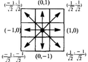
demonstrated successfully for generating a micro- drainage network from a set of DEM data, are unsuitable for generating drainage directions for a grid-based model such as AGNPS (a non-point source pollution model, described by Young and others, 1994), because approximating macro-scale trends from micro-variation data is difficult. For example, the DEM data used here have a pixel resolution 40 m x 40 m. Grid-based models, such as those used for water quality and regional planning, do not require such detailed topographical infor- mation. A typical cell size for AGNPS is 10 acres, which includes roughly 5 x 5 DEM pixels. The drainage direction of a grid cell is illustrated in Figure 2 is restricted to one of eight directions. Each direction points to an adjacent grid cell. The DEM data for micro-scale areas (pixels) are processed for approximating drainage trends of larger area, model grid cells. Unlike the research undertaken for a micro-scale drainage network, the micro-scale DEM
(2* (0,-l) (k* Figure 2. Possible drainage directions.
A neural network for grid pattern recognition 1037
(8 x
to,-
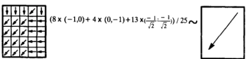
Figure 3. Micro-scale variation vs. macro-scale trend (vectorial average method).
data in this research are converted into macro approximations of drainage trends. An example of applying the vectorial average method (Kao, 1992b) is provided in Figure 3, in which a grid drainage direction was approximated from 25 pixel directions. Some difficulties may be encountered during such approximations. For example, Figure 4 shows two grid cells with the same vectorial average but with different spatial distributions of micro-scale pixel directions. The drainage directions of the two grid cells, if manually determined, obviously differ. Methods developed previously for determining micro-scale drainage network cannot be used directly for macro approximations because of such difficulties. The detail of micro-variation vs. macro- scale trend is discussed by Kao (1992a, and 1992b). Human judgment involved in determining the drainage directions from a topographic map is difficult to model mathematically or with a computer code. Therefore the neural network method with self-learning capability was explored.
Six methods were developed by Kao (1992a, and 1992b) to approximate a drainage pattern with a FORTRAN program. The drainage network method is demonstrated to be superior to other methods. The following discussion is focused therefore on compari- son of results obtained from the manual, drainage network and neural network methods. A subwater- shed within Chi-Mei Creek in North Taiwan serves as the test area. The area is divided into 1962 200 m x 200 m grid cells. All DEM pixels within the test area are divided into groups of 5 x 5 pixels; each group represents a typical model grid cell used for AGNPS.
Manual method
A manual method for creating a drainage pattern from topographical maps based on visual inspection was first imnlemented before testing other methods.
J
(A) (B)
Figure 4. Two grid cells with same vectorial average.
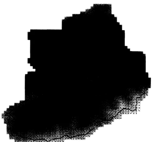
The manual method was performed using two approaches. One was carried out by placing grid cell boundaries on the maps, and grid cells were examined sequentially so as to determine their drainage directions manually. This process was, however, time consuming. In the second method a three-dimen- sional display, a contour figure, and an elevation- based figure were provided, and for each grid cell the major drainage direction was determined from the local grid cells. Inherent bias exists during the application of this method (see discussion in Kao 1992a, and 1992b). The drainage pattern so determined is illustrated in Figure 5. The darker area in the figure indicates lower ground, and vice versa. The three dark grid cells are outlets of the subwatershed. The subwatershed is encircled with a darkest line, which was digitized from topographical maps.
Drainage-network method
Each grid cell, in using this method, is treated as a small watershed. The first step is to determine the drainage direction of each DEM pixel. Allowing the drainage direction to drain towards the adjacent pixel with the lowest elevation is the simplest way to determine the pixel drainage direction. The outlet pixel is then determined on the basis of all pixel drainage directions within a composite grid cell. The drainage direction of the outlet pixel is then used as the drainage direction of the whole grid cell. If no outlet is found due to a depression pixel existing at a pixel within the grid cell, the pixel is then filled by re-setting its elevation to be slightly greater than that of the adjacent pixel with minimal elevation. This process is repeated until an outlet is found. This process was adopted from the Apparent Elevation method proposed by Yuan and Vanderpool (1986). The outlet pixel, however, may not be unique; having more than one outlet pixel within a grid cell is possible. If such a problem arises, the outlet pixel into which the greatest number of upstream pixels drain is chosen as the outlet. Discussion of the differences among the results obtained from this method and others are provided later.
NEURAL NETWORK DEMONSTRATION BY THE PROGRAM
Network configuration and hidden nodes
The neural network configuration tested (Fig. 1) is constructed of three layers: 25 input nodes, several hidden nodes, and eight output nodes. Each input
Figure 5. Manually determined drainage pattern
node is associated with a DEM pixel of a grid cell, and each output node is associated with one of eight drainage directions shown in Figure 2. Networks with 2, 3, 5, 8, 10, 13, 15, 18, 20, 23, 26, 29, 32, 35, 38, 41, and 44 hidden nodes were tested, as defined by the Per1 array @hiddenSet in the program.
Preparation of training sets
The selection of an appropriate training set is important for learning convergence and neural network performance. Of 1959 manually determined grid patterns, 160 grid patterns (less than 10%) were selected as a training set for the network. Training patterns were prepared in two sets as follows:
1. the entire grid cell set was divided into eight pools; the manually determined drainage direction of each grid cell in the same pool is the same;
2. grid cells are deleted from each pool if their drainage directions determined according to the manual and drainage network methods are not the same;
3. to form training set Dl, 20 grid cells were selected randomly from each pool;
4. repeat step (3) to form training set D2.
grid pattern. Other training sets such as those generated randomly from the entire grid cell set were tested also, but are not demonstrated here.
Normalization of input patterns
The normalization function shown in Equation (5) was used to compute the input value for each input node based on the associated DEM pixel elevation. Input values are between zero and unity.
I, = n1 - nmm *0.9 + 0.1
nmsr - nmin (5)
where I, is the final input value to an input node, n, = (e, - e~,.)/(e~,, - eP,,,)*O.9 + 0.1, e, is the el- evation of the current DEM pixel, ef,, is the minimum elevation of all pixels within the tested area, einx is the maximum elevation of all pixels within the area, n;,, is the minimum of n, and nkpx is the maximum of q’s
of the 25 pixels within the current grid cell. The network was sometimes not completely trained with the normalized value n,. Several obvious patterns, but with a small elevation, were observed to not be learned during many learning cycles. The magnitude The output node values lie between zero and unity. of the elevation appeared to be learned by the Only one output node of each training grid pattern network. The drainage pattern is governed primarily is set to unity; all others are set to zero. The node with by the pixel elevation variation rather than by the a nonzero output is associated with the drainage magnitude. The normalized function (Eq. 5) is thus direction assigned for the input pattern of the training proposed to enlarge the variation of a flat area.
A neural network for grid pattern recognition 1039
Direction and step methods
Direction and step methods in various combi- nations were tested (see the end of the program in Appendix 1 after START JOBS). The steepest descent method was tested for a step size equal to 0.1, 0.3, or 0.5 and the momentum-descent method was tested with a step size 0.1, 0.3, or 0.5, and decay rate 0.5, 0.7, or 0.9. In total 442 (2 training sets x 17 numbers of hidden nodes x 13) cases were tested according to steepest- and momentum-descent methods with fixed step sizes. Because these methods failed to learn the training set completely within 2000 iterations, the results are not reported here. These two methods were not tested further, because finding a good fixed step size is arbitrary, requires an extensive iterative procedure, and because the optimal solution may be missed. Only the methods of steepest descent (SD), conjugate gradient (CG), and Rudi’s conjugate (RC) gradient with line search generated satisfactory results.
Network training and results
Each input value is computed by the normalized function (Eq. 5). All training grid patterns are fed through the network once, and the link weights are modified at the end of each epoch. The values of
weights are not constrained. The network is trained in at most 2000 iterations (training stage). The 1959 grid drainage patterns of the test area are then determined by the trained network (validation stage). The drainage direction of each grid cell is set to be that associated with the output node with the maximum output value. All neural network training for this study was implemented with Xerion on a Sun Spare workstation with the following two commands.
nohup per1 doNet demNnet dem.trainDl dem.valid >& /dev/null&nohupperldoNet
demNnet1 dem. trainD2 dem.valid > & /dev/ null &
where dem. trainD1 and dem. trainD2 are names of files for the two sets of training cases, and dem.valid is the file name for the validation set. Several intermediate and summary files are created for each training and validation stage. The files include an input file to operate the Xerion bp module, a Xerion bp output file, a file to store link weight values, validation reporting files for training and validation sets, and a summary file. Table 2 shows an example of the Xerion bp input file created by the program for both training and validation stages. Table 3 shows a sample of the summary file for learning performance, validation performance, and CPU time usage. The summary file is created mainly Table 2. Sample Xerion bp input file created by program
# sample input for demNnetDI_12_cg.in used for the training stage. addNet “demNnetD1”
useNet “demNnetD1”
addGroup -type INPUT input 25 addGroup -type HIDDEN hidden 12 addGroup -type OUTPUT output 8 disconnectGroups “Bias” “input” ConnectGroups input hidden ConnectGroups hidden output
addExamples -type TRAINING dem.trainDl seed 120
randomize 1
set currentNet.extension.zeroErrorRadius = 0 minimize -tolerance l&e-IO -iter 5 -cg -epsilon 0.3 saveweights wt/demNnetDl_llcg.wt
exit
# sample input for demNnetDl_lLcg.inV used for the validation stage. open demNnetD1 > validate/demNnetD1_1Icgvalidate
format UnitRec.target “%7.4f’ format UnitRecoutput “%7.4f’ addTrace doExamples “print ”
(trace.fmt listed in Appendix 3 is included here.) @demNnetDl”
addNet “demNnetD1” useNet “demNnetD1”
addGroup -type INPUT input 25 addGroup -type HIDDEN hidden 12 addGroup -type OUTPUT output 8 disconnectGroups “Bias” “input” ConnectGroups input hidden ConnectGroups hidden output
addExamples -type TRAINING dem.trainDl loadweights wt/demNnetD1_12_cg.w addExamples -type VALIDATION dem.test doExamples -t VALIDATION
close demNnetDI
deletestream -quiet demNnetD1
open demNnetD1 r vaIidate/demNnetDl_ILcg.train doExamples -type TRAINING
close demNnetD1 exit
1040 J.-J. Kao
Table 3. Sample list of summary file created by program
Report for demNnetDL02steepestRay on 941025232212 TIME user = 188.3 sys = 2.3 real = 21 I .9
TIMEV user = 65.4 sys = 7.2 real = 78. I
iter= OnFE= If= 380.65738u= 1.2e+02d= -1,33e+O4dr= 1 iter = 2000 nFE = 2061 f = 65.805695 /g! = 0.77 d = - 0.741 dr = - 0.23 TDiff 0:124 45:35 9O:l 135:O 180:0 - > 160
VDiff 0:1032 45:785 90:106 135:32 180:4 _ > 1959...OK’?... Report for demNnetD1_02_cg_Ray on 941025232520
TIME user = 82.2 sys = 0.8 real = 88.5 TIMEV user = 65.4 sys = 5.9 real = 79.5
iter= OnFE= 1 f= 380.65738u= 1.2e+02d= -1.33e+04dr= 1 iter = 525 nFE = 893 f = 61.628765 u = 0.32 d = - 0.00542 dr = 1 TDiff 0:122 45:35 90:3 135:0 180:0 - > 160
VDiff 0:998 45:751 90:144 135:47 180:19 - > 1959...OK?... Report for demORG_OS_cgrudiRay on 941026000227
TIME user = 99.4 sys = 1.4 real = 107.3 TIMEV user = 64.8 sys = 5.8 real = 77.5
iter= 0 nFE= 1 f= 315.37115 I@1= 1.3e+02 d = - 1.62e+04 dr= 1 iter = 471 nFE = 689 f = 2.0000029 u = 3.5e - 05 d = - 9.3e - 07 dr = 1 TDiff 0:158 45:2 90:0 135:0 180~0 - > 160 Hmmm...Try further...
VDiff 0:1180 45:590 90~109 135:50 180:30 - > 1959...OK?...
by a user provided function call reportsub. A sample of reportsub for the case study is listed in Appendix 2 and its pseudocode is shown at the end of Table 1. The function compare called by reportsub is a problem-dependent function and must be modified if the problem is altered. This function compares the result from the validation stage with the desired one based on a comparison method provided by the user. The function appears complicated for this example because comparison of the results is not straightforward and requires data conversion from a numeric value to an angular value (unit: degree). For most problems that require direct comparison of numeric values, the function can be simplified significantly.
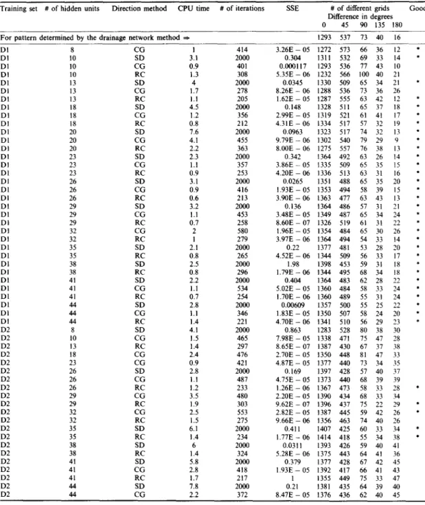
In total 102 (2 training sets x 3 methods (SD, CG, and RC) x 17 numbers of hidden nodes) cases, were trained. Table 4 shows all completely trained cases for each training set and method. A completely trained case is one that learns all the given training patterns within 2000 iterations. Cases with 2, 3, or 5 hidden nodes were unable to learn any of the tested training sets completely, consistent with the concept that more hidden nodes are required in learning a complex problem. The computation time and final errors for training the completely trained cases are summarized in Table 4. Comparisons are made on the basis of the difference between the computed and manual results reported according to the difference in the number of grid directions matching or 45“, 90’, 135”, or 180”. 1293 grid cells exactly match the manually determined ones, 573 grid cells have a 45’ difference, 73 grid cells have a 90” difference, 40 grid cells have a 135” difference, and sixteen grid cells have a 180” difference. Grid cells at a 45’ difference from the manually determined results may arise because during the manual process one or two alternative adjacent directions are observed frequently. Grid cells
with a 45” difference from manual ones therefore are considered acceptable. There are 36 cases in which the computed and manual methods were different. However, this number was reduced greatly if directions off by 45” were considered acceptable.
CONCLUSION
Researchers seek automated methods for imple- menting conventional modeling tasks. A neural network with self-learning and self-organization capability is a promising technique to replace tasks that involve human judgment. The Per1 program developed in this work is intended to relieve the burden on an analyst from implementing the conventional iterative neural network training pro- cedure and research result reporting. A complex test such as the study demonstrated here can be implemented with a small number of nohup commands.
The result obtained from the neural network method applied to a case study is satisfactory in comparison to the manually determined drainage pattern, and is superior to other previously developed numerical methods. The selection of appropriately balanced training sets, sufficient hidden nodes, a suitable normalization method, and the best direction methods are the major factors in building an efficient neural network. These factors are explored readily with the program which can be executed in a background mode. With slight modification the program can be applied to explore neural network research of other types. All programs, including several data and report processing scripts developed in this work are available for public accesses. Information for obtaining them can be requested by e-mail addressed to [email protected]., or by anonymous FTP from IAMG.ORG.
A neural network for grid pattern recognition 1041 Table 4. Completely trained cases
Training set # of hidden units Direction method CPU time # of iterations SSE # of different grids Good Difference in degrees 0 45 90 135 180 For pattern determined by the drainage network method *
- DI DI Dl DI Dl DI DI Dl DI Dl Dl Dl DI DI Dl DI DI DI Dl DI Dl DI Dl DI Dl Dl Dl Dl DI Dl Dl DI Dl DI D2 D2 D2 D2 D2 D2 D2 D2 D2 D2 D2 D2 D2 D2 D2 D2 D2 D2 D2 D2 D2 8 CG IO SD IO CG IO RC I3 SD I3 CC 13 RC 18 SD I8 CG 18 RC 20 SD 20 CG 20 RC 23 SD 23 CG 23 RC 26 SD 26 CG 26 RC 29 SD 29 CG 29 RC 32 CG 32 RC 35 SD 35 RC 38 SD 38 RC 41 SD 41 CG 41 RC 44 SD 44 CG 44 RC 8 SD 10 CG 13 RC I8 CG 23 CG 26 SD 26 CG 26 RC 29 CG 29 RC 32 CG 32 RC 35 SD 35 RC 38 SD 38 RC 41 SD 41 CG 41 RC 44 SD 44 CG I 3.1 0.9 1.3 4 1.7 I.1 4.5 I.2 0.8 7.6 4.1 2.2 2.3 1.1 0.9 3.1 0.9 0.6 3.2 1.1 0.7 2 1 2.1 0.8 2.5 0.8 2.2 1.1 0.7 2.8 1.1 I.4 4.1 1.5 1.4 2.4 0.9 2.8 1.1 1.2 3.5 1.9 2.5 1.5 6.1 1.4 6 1.4 5.8 2.8 1.7 7.8
Acknowledgments-The author thanks Mr C. H. Tsai and Mr S. F. Bau for assistance in determining drainage pattern from DEM data manually, the National Science Council of Taiwan R. 0. C. for providing partial financial support (NSC 82-0410-E-009-18), and to Camp, Plate, and Hinton (1993) for providing Xerion; without it, complicated research such as the case study could not be achieved with only two simple nohup commands.
REFERENCES
Aho, A. V., Kerninghan, P. J., and Weinberger, P. J., 1988, The AWK programming language: Addison-Wesley, Massachusetts, 210 p. 414 2000 401 308 2000 278 205 2000 356 212 2000 455 363 2000 357 253 2000 416 213 2000 453 258 580 279 2000 265 2000 296 2000 534 254 2000 346 221 2000 465 297 476 421 2000 487 233 480 303 553 275 2000 234 2000 324 2000 418 217 2000 372 1293 537 73 40 16 3.26E - 05 1272 573 66
69
36 I2 0.304 1311 532 33 14 0.000117 1293 536 77 43 IO 5.358 - 06 1232 566 loo 40 21 0.0345 1330 509 65 34 21 8.26E - 06 I288 536 73 36 26 1.62E - 05 I287 555 63 42 12 0. I48 1328 511 65 37 I8 2.99E - 05 1319 521 61 41 17 4.31E - 06 I334 517 57 32 19 0.0963 1323 517 74 32 13 9.79E - 06 1302 540 79 29 9 8.OOE - 06 1275 557 76 38 13 0.342 I364 492 63 26 14 3.86E - 05 I335 509 65 35 I5 4.20E - 06 1336 513 63 31 I6 0.0265 1351 488 65 35 20 l.93E - 05 1353 494 58 39 15 3.90E - 06 I363 477 63 43 13 0.136 1364 486 51 31 21 3.488 - 05 I349 487 65 34 24 8.60E - 07 I326 519 61 31 22 1.96E - 05 I354 484 65 30 26 3.97E - 06 1364 494 54 33 14 0.22 1377 481 53 28 20 4.52E - 06 1344 509 56 33 17 1.98 I398 453 59 31 18 1.79E - 06 1344 495 68 34 18 0.404 1364 483 62 28 22 5.02E - 05 1360 484 58 33 24 I .70E - 06 1360 489 55 31 24 0.00609 1357 500 55 25 22 l.83E - 05 1350 507 58 24 20 4.70E - 06 1341 510 56 29 23 0.863 1283 528 80 38 30 7.988 - 05 1338 471 75 47 28 8.658 - 07 1387 430 61 37 38 2.70E - 05 1350 448 81 47 33 4.87E - 05 1377 440 73 34 35 0.169 1397 428 57 40 37 4.758 - 05 1373 440 68 39 39 1.26E - 06 1367 473 58 33 28 2.20E - 05 1390 434 68 33 34 9.628 - 07 1396 437 75 22 29 2.82E - 05 1387 445 59 42 26 9.66E - 06 1356 463 74 40 26 0.411 1407 425 60 33 34 I .77E - 06 1414 418 55 34 38 0.031 I I393 426 59 40 41 5.28E - 06 1375 443 64 41 36 0.379 I377 428 67 42 45 I .93E - 05 1392 417 66 41 43 1355 449 75 33 47 0.21 1381 435 64 39 40 8.478 - 05 1376 436 62 40 45Band, L. E., 1986, Topographic partition of watersheds with digital elevation models: Water Resources Research, v. 22, no. 1, p. 15-24.
Burrough, P. A., 1986, Principles of geographical infor- mation systems for land resources assessment: Clarendon Press, Oxford, 194 p.
Camp, D., Plate, T., and Hinton, G., 1993, The Xerion neural network simulator version 3.1: Department of Computer Science, Univ. Toronto, 43 p.
Kao, J.-J., 1992a, Determining drainage pattern using DEM data for nonpoint source water quality modeling: Final Report to National Science Council, Taiwan, R. 0. C. (NSC 80-0410-E-009-18), 84 p.
Kao, J.-J., 1992b, Determining drainage pattern using DEM data for nonpoint source water quality modeling:
1042 J.-J. Kao Water Science and Technology, v. 26, no. 56, p. 1431-1438.
Mirchandani, G., and Cao, W., 1989, On the hidden nodes for neural nets: IEEE Trans. Circuits and Systems, v. 36, no. 5, p. 661-664.
O’Callaghan, J. F., and Mark, D. M., 1984, The extraction of drainage networks from digital elevation data: Computer Vision, Graphics, and Image Processing, v. 28, p. 324-344.
Press, W. H., Teukolsky, S. A., Vettlerling, W. T. and Flannery, B., 1992, Numerical recipes in C: Cambridge University Press, New York, 994 p.
Rumelhart, D. E., McClelland, J. L., and the PDP research
group, 1989, Parallel distributed processing: MIT Press, Cambridge, Massachusetts, 547 p.
Wall, L., and Schwartz, R. L., 1992, Programming Perl: O’Reilly and Associates, Inc., California, 465 p. Yuan, L. P., and Vanderpool, N. L., 1986, Drainage
network simulation: Computers & Geosciences, v. 12, no. 5, p. 653665.
Young, R. A., Onstad, C. A., Bosch, D. D., and Anderson, W. P., 1994, Agricultural non-point source pollution model, version 4.03, AGNPS user’s guide: US Dept. Agriculture-ARS North Central Soil Conservation Research Laboratory, Morris, Minnesota, 112 p.
APPENDIX 1
Program doNet
#!/usr/local/bin/perl Script name: doNet
Purpose : Implement batch Neural Network trainings using Xerion/bp. Computation time is computed by Unix command ‘time.’ Tested successfully on SunOS4.l.x and HPUX 9.02. Author: Jebng-Jung Kao [email protected]
ftp site: ftp.edu.tw:/misc/environment/NCTU_HV/nnet/doNet evOOs.ev.nctu.edu.tw:/nnet/doNet
Last updated on 03/10/1995.
Variable sets to be predefined by the user. ~hiddenSet~("02~~,"05","08","11","14","17"
# number of nodes in the hidden layer. ’
"20*~ 88231t "2508, 182g8$, "328:. 0035<*, ";*w,) ; ’
Default values for optional user-specified variables. $traceFMTfile="trace.fmt";
$reportsub=flreport.sub'Q. # user defined subroutine for producing reports $reportFile="report/Summary";
Default values for problem dependent variables. $inUnitNum=49;
$outUnitNum=S;
# $rep="l"; # if you need information for every $rep iterations. $iter="2000";
# Problem independent variables(well! you can change them also.) $seed=llO;
$randomize=l.O;
#$weightCost=$l; #if set, minimize error with network cost errors $zeroErrorRadius=O;
$doExamples="VALIDATION"; $doMinimize="yes";
# Command path which may be system-dependent; $MVBIN="/bin/mv"
$MKDIRBIN=*1/bin/mkdir80; $TIMEBIN="time".
SXBRION_BPBIN=~~~~~~; $MAILCMD="/usr/ucb/Mail";
# for hpux, $MAILcMD=q8/usr/bin/mailx"; $RMBIN="/bin/rm";
$LNBIN="/bin/ln";
# Tag character for validation path. $validateTAG='QV't;
$usage="Usage: donet netName trainFile validateFile (in# out#l"; if($#ARGV != 2 && $#ARGV != 4) { print "$usage\n"; exit;} $netName=$ARGV[O]; $trainFile=$ARGV(l]; $validateFile=$ARGV(2]; if ($#ARGV == 4) { $inUnitNum=$ARGV[3]; $outUnitNum=$ARGV(4] ; )
# Check file and directory existence. if (! -s StrainFile) {
print "Error: Training Set file StrainFile does not exiSt.\n$USage\n"; exit;
if (! -s print exit; 1 if (! -d print
A neural network for grid pattern recognition
$validateFile) (
"Error: Validation Set file $validateFile does not exist.\n$usage\n";
$netName) (
"Creating directory SnetName/ . ..\n". ~~~~.
system("$MEDIRBIN SnetName") ; }
chdir($netName) ; if(! -s "$trainFile") {
print "Linking StrainFile to SnetName/ . ..\n". system("$LNBIN -s ../$trainFile StrainFile"); J
if(! -s 08$validateFile") (
print "Linking $validateFile to SnetName/ . ..\n". system("$LNBIN -s ../$validateFile SvalidateFile") ; 1
if(! -s U ../$traceFMTfile") ( $traceFMTfile="";
print "Warning: no trace format file. No trace done.\n"; ) elsif (! -s "$traceFMTfile")(
print "Linking $traceFMTfile to SnetName/ . ..\n". system("$LXBIN -s ../$traceFMTfile StraceFMTfile"); 1
user-provided reporting file. if(-s U ../$reportsub")(
# if you want to keep different version of the report file, pls. # uncomment the following 5 lines.
# if(-s $reportFile) { : $thistime=‘date +%y%m%d%?i%MtS‘; chop($thistime); # # 1
system("$MVBIN $reportFile $reportFile.$thistime"); if(! -s "$reportsub") {
print "Linking Sreportsub to SnetName/ . ..\nl'. \ system("$LNBIN -s ../$reportsub Sreportsub");
I donot want to see display in batch training, # but it is useful for interactive training. $ERV(*DISPLAY')="/dev/null~;
Create a TAG file for which run is being implemented. $home=$ENV{'HOME'};
$hostname=‘hostname‘; chop($hostname);
if ( ! -d "$home/tmp" ) ( system("$MRDIRBIN $home/tmp"); ) $tagFile="$home/tmp/donet$user$netName$hostname";
create required directories.
@needDirs=("in","wt","validate","out","report"); foreach $d (@needDirs)( if (! -d Sd) { system("mkdir $d") ; 1 1 1043
if(-s $reportsub) ( require Sreportsub;}
1044 J.-J. Kao
sub doNet(
# set name=$netName ShiddenUnitNum ($cg($method}[_$epsilon[_$alphall I_$lsl SthisRunName=VS(netNameJ ShiddenUniENum":
if($method eq A;) { # non~momentum and non-steepest-decent method $thisRunName="$(thisRunWame)_$cg";
} else (
$thisRunName="$(thisRunWame} Smethod";
if($epsilon ne "") ( $thigRunName=" $(thisRunName}_$epsilon"; } if($alpha ne "") ( $thisRunName="$(thisRunName)_$alpha"; ) if($ls ne ~~ )($thisRunName="$(thisRunName)_$ls");
# set input/output file names.
$weightFile="wt/$thisRunName.wt"; # weight
$loadWeights=$weightFile; # re-load weight
$validateOutputFile="validate/$thisRunName.validate"; # validation $trainOutputFile="validate/$thisRunName.train"; # training $bpInFile="in/$thisRunName.in"; # bp input $bpOutputFile=~80ut/$thisRunName.bp"; # bp output $timeReportFile=@lreport/$thisRunName.time'D; # time report
# create a TAG to keep track where it is, when running background. system("echo I am doing this case:$thisRunName now. >$tagFile");
# notify the user; NOTE: you may receive too many message. # if you want to reduce, you may move this line after dolet.
system("$MAILCMD -s \O'$thisRunName$hostname\'V $email_address <StagFile"); # training
$validateIt=OV";
&writeNetIn($bpInFile,""J ;
system("$TIMEBIN $XERION BPBIN c$bpInFile$validateIt l>$bpOutputFileSvalidateIt 2>$timeReportFile$validateIt7);
# validation
$validateIt=$validateTAG;
&writeNetIn($bpInFile,$validateIt); system(
8V$~~~~~~ BPBIN <$bpInFile$validateIt i>$bpOutputFileSvalidateIt Z>/dev/null") # In most case, validation is quick and no need to report.
# system("$TIMEBIN $XERION_BPBIN <$bpInFile$validateIt 1~SbpOutputFileSvalidateIt 2>$timeReportFile$validateIt");
# execute user-specified reporting, if provided if(-s Sreportsub) (
&reportsub($thisRunName,$bpOutputFile,$timeReportFile,$trainOutputFile.$validateOut putFile,$reportFile) ;
# This function write a XERION input file. You may consult XERION manual to # modify it to meet your needs.
sub writeNetIn{
local($netInFile,$validateIt)=@_;
#print "Writing $netInFile, please wait...\n"; open(NETIN,">$netInFile$validateIt') 1 )
die "Error:canot open $netInFile$validateIt $!\n"; if($validateIt eq $validateTAG) ( # validation phase
if($validateOutputFile ne "") {print NETIN "open $netName > $validateOutputFile\n';J if($UnitRectarget ne "I') (print NETIN
"format UnitRec.target \"$UnitRectarget\"\n";) if($UnitRecoutput ne 'I") {print NETIN
"format UnitRec.output \"$UnitRecoutput\"\n";} if($traceFMTfile ne "") {
A neural network for grid pattern recognition $count{$diffDegree}++;
)
$test_validEntry=cTEST_VALID>; # ignore blank lines close(TEST VALID);
# report t&al # of cases, if desired. should be = $matchcount # print "TOtal=$totalcount\n";
$matchcount=o;
foreach $d (@degreeList){ Smatchcount += $count($d}; } # set flag for success
$success=~'~8; # best result;
if($count{'O'} == $totalcount){$success== Yu...Hoo...";} # for training set, < 5 untrained case; marginally trained.
elsif(($totalcount-$count('0'j) < 5) ($success=fl Hmmm...Try further...";} # for validation set, 0+45 > 1350 cases is acceptable.
elsif(($count('O')+$count('45')) > 1350)($success=" . ..OK?...".) # report the summary.
print REPORT 8 TDiff\tO:Scount('O') 45:$count{145') 90:$count{190*) 135:$count('135') IBO:$count('l80~) -> $matchcount$success\n";
1045
close(REPORT);
if($success eq "") ( return "0";) # bad case return #'II;
1
# This function extract time information from Unix time command output. sub timeOSdep (
local($OSNAME,$timeReportFile)=@ ; local($systime,$realtime.Suserti~e); open(TIME,"$timeReportFile');
# SunOS's and HP-UX's 'time' while (<TIME>) (
commands produce slightly different output. if ($oSNAME eq "SunOS") (
if(/^[ \t]+([\w.]*) [ \tl+realI \tl+(I\w.l*) [ \tl+user[ \tl+([\w.l*) 1 \tl+sYs/) I $realtime=$l;
$usertime=$2; $systime=$3; )
) elsif ($OSNAME eq "HP-UX") (
if(/^sys[ \tl+([\w.l*) [ \tl*/) ($systime=Sl) if(/^real[ \tl+([\w.l*) [ \tl*/) if(/^user[ \tl+([\w.l*) [ \tl*/) 1 I $realtime=$l $usertime=Sl I else {
print "Hmmm... I donot know your OS: SOSNAME\n"; return (-1,-1,-I);
1
\ # YOU may add other OS dependent code here, if applicable system("$RMBIN -f $timeReport"); #NOTE SRMBIN is defined in doNet )
return ($systime,$realtime,$usertime);
# Function called by doNet for user-specified reporting. sub reportsub(
# get OS name for 'time' command output format. if ($uname eq "")(
$uname=‘uname -a‘; chop($uname); 1
if ($uname =-/^([\w-I*) [ \tl+/) { $thisOS=Sl)
0~633 (REPORT, ">>$reportFile"); # get system date/time.
$thistime='date +%y%m%d%H%M%S‘; chop($thistime); print REPORT "Report for SentryName on $thistime\n*;
# if $timeReport file exists, extract time and add it into the summary. if(-s "$timeReport") (
($systime,$realtime,$usertime~=&timeOSdep~$thisOS,$timeReport~;
print REPORT 'I TIME\tuser=$usertime\tsys=$systime\treal=$realtime\n~~; I
# if time report file for validation phase exists, summary it also.
#In most case, validation is quick, and no need to report it. see doNet. #NOTE: $validateTAG is defined in doNet.
if(-s "$timeReport$validateTAG") (
($systime,$realtime,$usertime)=&timeOSdep~$thisOS,"$timeReport$validateTAG"~; print REPORT " TIMEV\tuser=$usertime\tsys=$systime\treal=$realtime\n~1; )
# try to get 1st and last Iter lines.
# YOU may edit function getIter for this purpose. if( -s $bpOut) {
&getIter($entryName,$bpOut) ; $firstIter='head -1 $bpOut';
if($firstIter ne "") ( print REPORT ' $firstIter";} $lastIter=‘tail -1 $bpOut‘;
if($lastIter ne "") ( print REPORT ' $lastIter";}
system("$RMEIN -f $bpOut"); #NOTE: $RMBIN is defined in doNet. system("$RMBIN -f $bpOut$validateTAG");
I
# ________-_---Specific steps for DEM case _--__--__--__ # check training results.
# if the Nnet configuration produce acceptable result, return ""; # otherwise $lastFlag will return "D"
$lastFlag=hcompare($trainOut,$reportFile) ;
$lastFlagl="D"; # kill all files, anyway, to save space if($lastFlag == "DW) { system("$RMBIN -f $trainOut"); system('$RMBIN -f in/$entryName.in"); system("$RMBIN -f in/$entryName.in$validateTAG"); system(19$RMBIN -f wt/$entryName.wt"); I
# check validation results.
# if the Nnet configuration produce acceptable result, return ""; # otherwise $lastFlag will return "D"
$lastFlagl=&compare($validateOut,$reportFile) ; $lastFlagl="D"; # kill all files
if($lastFlagl == "D'@) ( I anyway. to save space system(81$RMBIN -f $validateOut"); if( $lastFlag eq "") { system(3'$RMBIN -f $trainOut") ; system("$RMBIN -f in/$entryName.in"); system("$RMBIN -f in/$entryName.in$validateTAG"); 1 system("$RMBIN -f wt/$entryName.wtt8); I
A neural network for grid pattern recognition APPENDIX 2
Sample report. sub
# --- START of report.sub included by doNet--- # This is a sample file for report.sub for running doNet. # Case description: DEM Drainage Network training. # Author: Jehng-Jung Kao [email protected] # ftp site: ftp.edu.tw:/misc/environment/NCTU_EV/nnet/donet # Last updated on 03/10/95.
# This function keep only lines with ^iter= from Sthefile, XERION/bp output. sub getIter(
local($entryName,$thefile)=@_; local($tmpfile)="/tmp/junk$entryName"; open(THEFILE,"$thefile");
open(TMPFILE,">$tmpfile");
while (<THEFILE>) { if (/^iter= /) {print TMPFILE $_;)} close(TMPFILE); close(THEFILE);
system("$MVBIN $tmpfile $thefile"); #NOTE SMVBIN is defined in doNet
IO47
# List of degrees to be reported for differences. @degreeList=('O','45','90','135','180');
# This function compare training or validating DEM drainage pattern results sub compare{
local($test_validOutFile,$reportFile)=@_; if(! -6 $test_validOutFile) (return;) # Initialization.
open(R~P0~~, ">>$reportFile"); open(TEST_VALID,$test_validOutFile);
$totalcount=O; # count total # of cases. foreach $d (@degreeList){ $count($d)=O; } # Do comparison for reporting difference. while (<TEST-VALID>) (
$totalcount++;
# delete leading blanks
$test_validEntry=$_; chop($test_validEntry) ; $test_validEntry =_ s/* [ \tl*//; # split into a List
@targetList=split(/[ \tl+/,$test_validEntry); # find the target direction, with maximal value. Smax=O.O:
_---- ,
for($i=O; $i < 8; $i++){
if ($targetList [$il > $max) (Smax=$targetList [Sil ; \
$targetDir=$i+l;) .$targetDegree=($targetDir-1)*45;
# find the Nnet determined direction, with maximal value. $test_validEntry=cTEST VALID>; chop($test_validEntry); $test_validEntry =- s/~[ \tl*//; # delete leading blanks. @test_validList=split(/[ \tl+/,$test_validEntry);
$max=O.O;
for($i=O; $i < 8; $i++){
if($test_validList[$il > $max) {$max=$test_validList[$il ; 1
$test_validDir=$i+l;}
$test_validDegree=($test_validDir-1)*45; # compute the difference and count
$diffDegree=$targetDegree-$test_validDegree; if($diffDegree < 0) ($diffDegree=-SdiffDegree;} if($diffDegree > 180) ($diffDegree=360-$diffDegree;-)
1048 J.-J. Kao
if (! -s $traceFMTfile) {print "Error: $traceFMTfile is empty.\n";exit;) print NETIN "addTrace doExamples \"print \I\"';
open(TRACEFMTFILE,"$traCeFMTfile");
while (cTRAcEFMTFILE>) (print NETIN "\t$_";) close(TRACEFMTFILE);
print NETIN "@$netName\"\n"; 1
I
print NETIN "addNet \"$netName\"\n"; print NBTIN "useNet \"$netName\"\n";
if($inUnitNum eq "") ( print "Error: no inUnitNum.\n"; exit} print NETIN "addGroup -type INPUT input $inUnitNum\n";
if($hiddenUnitNum eq "") ( print "Error: no hiddenUnitNum.\n"; exit] print NETIN "addGroup -type HIDDEN hidden $hiddenUnitNum\n";
if($outUnitNum eq "I') { print "Error: no outUnitNum.\n"; exit) print NETIN "addGroup -type OUTPUT output $outUnitNum\n"; print NETIN "disconnectGroUpS \"Bias\" \"input\"\n"; print NETIN flconnectGroups input hidden\n";
print NETIN "coMectGrOUpS hidden OutpUt\n";
if($trainFile ne 'I") (print NETIN "addExamples -type TRAINING $trainFile\n";) fi && $validateIt ne $validateTAG) { # training phase ~:~~~~!$i~?~f)eq "g?nt NETIN "seed $seed\n";}
if($randomize ne ""1 ( print NETIN "randomize $randomize\n";}
if($weightCost ne @'") ( print NETIN "set currentNet.weightCost = $weightCost\n";} if($zeroErrorRadius ne "") { print NETIN
"set currentNet.extension.zeroErrorRadius = $zeroErrorRadius\n";} print NETIN "minimize -tolerance l.Oe-10";
if($rep ne 18t0) ( print NETIN I' -rep $rep";} if($iter ne "I*) ( print NETIN II -iter $iter";) if($method ne "") ( print NETIN 'I -$method";
if($method eq "quickprop" && $1~ eq "")(print NETIN ' -qpEpsilon 0.1";) 1
if($cg ne "") ( print NBTIN 'I -$cg";)
if($epsilon ne "") ( print NETIN 'I -epsilon $epSilOn”;}
if($alpha ne 8t") ( print NETIN " -alpha $alpha";) if($ls ne "") ( print NETIN I( -ls$ls";}
print NETIN *'\n";
if($weightFile ne "") ( print NETIN "saveweights $weightFile\n";} 1
if($validateIt eq SvalidateTAG) (
if($loadWeights ne "") ( print NETIN "loadweights $loadWeights\n";} if($validateFile ne "") (print NETIN
"addExamples -type VALIDATION $validateFile\n";}
if($doExamples ne 'I") (print NETIN "doExamples -t $doExamples\n";} print NBTIN 10close $netName\n";
print NETIN "deleteStream -
if($trainOutputFile ne "") print NBTIN 7" iet $netName\n";
"open $netName > $trainOutputFile\n";) if($trainFile ne I"*) (print NETIN "doExamples -type TRAINING \n";}
print NBTIN tOclose $netName\n"; I
print NETIN "exit\n";
close (NETIN);
I
#___________ST~T JOBS_______________________________ foreach Sh (@hiddenSet) (
# repeat for number of hidden nodes = Sh. $hiddenUnitNum=$h;
# START OF USER SPECIFIED TRAINING STRATEGIES # steepest method -epsilon [0.310.5] and -1sRay
$ls=""; # line search method $cg= 1’ ” ;
$method="steepest". $epsilon="0.3"; ’
# only one can be non-null string # for step size 0
&doNetO; $epsilon=*0.5"; &doNetO ;
A neural network for grid pattern recognition $epsilon=""; # for step size 0
$ls=OURayU. &doNetO ;’
# momentum method -epsilon [0.110.3] -alpha [0.9/0.71 $ls~"~~; $method="momentum";
$alpha="0.9"; # for momentum method $epsilon="O.l"; # for step size &doNetO ;
$epsilon="0.3"; # for step size &doNetO ;
$alpha="0.7"; # for momentum method $epsilon="O.l"; # for step size &doNetO ;
$epsilon="0.3"; # for step size &doNetO ;
# Conguate Gradient method
$cg=*@cg81; $method=""; # only one can be non-null string &doNetO ;
# Rudi's Conguate Gradient method
$cg="cg8@; $method=""; # only one can be non-null string $cg=l*cgrudi"; &doNetO ; $cg='tcgRestart"; &doNetO; system("$RMBIN -f StagFile"); 1049 APPENDIX 3 Sample trace. fmt currentNet .group[3l.unit[Ol.target \ currentNet.group[3l.unit[1l.target \ currentNet.group[31.unit[21 .target \ currentNet.group~3l.unit~3l.target \ currentNet.group[3].unit[4l.target \ currentNet.group[31.unit[Sl.target \ currentNet.group[31.unit[6l.target \ currentNet.group[3] .unit[7].target currentNet.group[31 .unit[l].output \ \"\n\" currentNet.group[3l.unitIOl.output \ currentNet.group13l.unit[2l.output \ currentNet.group[3l.unit[3l.output \ currentNet.group[31 .unit[Ql.output \ currentNet.group[3l.unit[Sl.output \ currentNet.groupL3l.unitL61 .output \ currentNet.group[31 .unit[7].output \ \"\n\"\