國立交通大學
電信工程學系
博士論文
交錯耦合微帶線濾波器的調整與診斷
Tuning and Diagnosis of Cross-Coupled Microstrip Filters
研究生:廖竟谷 (Ching-Ku Liao)
指導教授:張志揚 博士 (Chi-Yang Chang)
交錯耦合微帶線濾波器的調整與診斷
Tuning and Diagnosis of Cross-Coupled Microstrip Filters
研 究 生:廖竟谷 Student:Ching-Ku Liao
指導教授:張志揚 Advisor:Chi-Yang Chang
國 立 交 通 大 學
電 信 工 程 學 系
博 士 論 文
A Dissertation Submitted toDepartment of Communication Engineering College of Engineering
National Chiao Tung University in Partial Fulfillment of the Requirements
in
Communication Engineering June 2007
Hsinchu, Taiwan, Republic of China
交錯耦合微帶線濾波器的調整與診斷
研究生:廖竟谷
指導教授:張志揚博士
國立交通大學電信工程學系﹙研究所﹚博士班
摘要
本論文主要在研究如何萃取交錯耦合濾波器之等效電路參數,進而調整濾波器使其 達到預先設定之響應。一般而言,交錯耦合濾波器之等效電路參數可由一個耦合矩陣來 表示,文中將對耦合矩陣的萃取與合成方法有詳盡的討論。同時文中也提出了系統化的 設計與調整濾波器的步驟。而這樣的方法與步驟可有效地用來分析微帶線濾波器中的交 錯耦合效應、共振腔頻率校正等問題。其中,對於具有源級與負載相耦合(source-load coupling)的四角互耦(quadruplet)結構有詳盡的討論。此外,文中也提出了如何快速 設計具高止帶頻率選擇性的串接三角互耦(cascade trisection)濾波器。除了在單模濾 波器的應用外,文中也深入探討了如何混用單模與雙模共振腔來實踐具廣義查比雪夫響 應之似盒狀(box-like)耦合濾波器。另外,文中也提出了一種新的參數萃取法,此法可 以從濾波器的響應同時萃取出耦合矩陣與無外加負載之品質因子(unloaded quality factor)。此種參數萃取法可以實際用於有損濾波器的分析與調整。Tuning and Diagnosis of Cross-Coupled Microstrip Filters
Student: Ching-Ku Liao Advisor: Dr. Chi-Yang Chang
Department of Communication Engineering
National Chiao Tung University
Abstract
This Dissertation presents how to extract the equivalent circuit parameters of cross-coupled filters. From the extracted parameters, one can decide how to tune a filter to achieve the prescribed response systematically. In most cases, the cross-coupled filters can be described by a coupling matrix. Thus, how to extract and synthesize a coupling matrix with a given response would be discussed in detail. Besides, a systematical procedure for filter design and tuning is given. With these developed methods, one can effectively analyze the effect of cross couplings and asynchronous resonant frequencies of resonators in microstrip filters. As an example, the quadruplet filters with source-load coupling are discussed in detail. And a cascade trisection filter with high selectivity in upper stopband is proposed. In addition to the design of single-mode resonator filters, we investigate how to utilize the dual-mode resonator with single-mode resonators to realize box-like filters with generalized Chebyshev response. To extract a coupling matrix and an unloaded quality factor of a filter from a simulated/measured response simultaneously, a novel parameter extraction method is proposed. This parameter extraction method can be used to analyze and tune lossy filters.
誌
謝
生命中,總有要做決定的時刻。當然,有些事情容易決定,有些則很困難。對我, 選擇讀博士班並不是個容易的決定。選擇讀博士班是對研究的憧憬、對未知事物的好 奇。但在現實的生活中,研究會有困難,親人也未必支持自己走研究這條路。周遭不少 人對我說過:『幹嘛念博士啊?』,『你做這有啥用,還不如去賺錢。』之類的話。但對 我而言,念博士班的人總有一個夢,有著對未知事務的好奇,而這樣的好奇心與想做出 點新奇的東西的想法驅動著自己去做研究。拿到博士學位並不是夢想的實現,而是一個 小里程的結束。 我要特別感謝張志揚教授的指導。張教授的開朗與耐心以及對專業知識的熟稔,對 於研究工作的進展有莫大的助益。在新竹的這幾年,叔叔嬸嬸的照顧以及可愛的堂弟堂 妹們的陪伴,讓我在研究之餘有精神上的調劑。在佛羅里達大學的期間,常志、政寧、 明旗、天宇的友誼,讓身在美國的我能快樂度日。在美國的期間,何雲幫了我許多忙、 教了我許多事情,他的幫助讓我能很快適應在美國的生活。Bruce 帶我認識了美國同時 拜訪了很多地方。 Linsay 則是最樂於糾正我的破英文的一位,我英文如有進步多要歸 功於他。林仁山教授夫婦熱心的幫忙與招待讓身在異鄉的我倍感溫暖。很高興有這麼多 人陪我走過這個里程。 廖竟谷 於交大 民國九十六年六月
Contents
Abstract (Chinese)………..Ⅰ Abstract (English) ………Ⅱ Acknowledgements………Ⅲ Contents………Ⅳ List of Tables………..Ⅵ List of Figures………Ⅶ Chapter 1 Introduction……….11.1 Review of the Design of Cross-Coupled Resonator filters………..2
1.2 Motivation………4
1.3 Literatures Survey………6
1.4 Contribution……… 9
1.5 Organization………10
Chapter 2 Design and Optimization of Microwave Filter Based on Coupling Matrix 2.1 Filter Model in the Normalized Domain ………13
2.2 The Position of Finite Transmission Zeros……….15
2.3 Synthesis Methods for Cross-Coupled Filters………17
2.4 Obtaining a Initial Design for a Microwave Filter………... 21
2.5 Tuning Procedures………..22
2.6 The Optimization Flow of Cross-Coupled Microwave Filters………...25
2.7 Limitations of the Proposed Design Flow………...28
Chapter 3 Cross-Coupled Filters with Source-Load Coupling 3.1 Introduction………... 29
3.2 Asymmetric Frequency Responses………32
3.3 CAD Methods for Filter Diagnosis……….35
3.4 Filter Design Examples………...38
Chapter 4 Modified parallel-coupled filters with two independently controllable upper stopband transmission zeros 4.1 Motivation ………...49
4.2 Circuit Description and Design Feasibility……….52
Chapter 5 Microstrip Realization of Generalized Chebyshev Filters with Box-Like Coupling Schemes
5.1 Introduction……….56
5.2 Circuit Modeling……….59
5.3 Design Examples and Experimental Results……….72
5.4 Discussion ………..76
Chapter 6 Parameter Extraction Method Based on Vector Fitting Formulation 6.1 Introduction……….78
6.2 Review of the Vector Fitting Technique……….81
6.3 Applying Vector Fitting to Parameters Extraction……….82
6.4 Example………..84
Chapter 7 Summary and Future Work 7.1 Summary……… 87
7.2 Future work……….88
List of Table
Table 2.1. Coupling topologies and the position of their corresponding finite transmission zeros………..…17
Table 5.1. Electrical parameters corresponding to box-section filters shown in Fig. 7(b).
Here,ϑC1 =90o,
o C2 =60
ϑ , Z1 =50ohm, Z2 =50ohm. All of the electrical lengthes are corresponding to the center frequency of the filter.
Design 1: in-band return loss RL=20dB, Ω=−2.57, and FBW=5% Design 2: in-band return loss RL=20dB, Ω=2.57, and FBW=5%
List of Figures
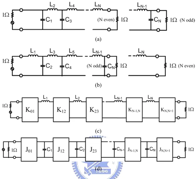
Figure 1-1 (a), (b) Lowpass prototype networks for “all-pole” filters. (c), (d) Alternative
lowpass prototype networks using inverter……….2
Figure 1-2 A cross-coupled resonator filter………...………...3
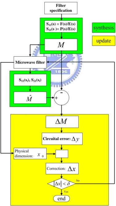
Figure 1-3 Flow diagram of the filter optimization algorithm………..7
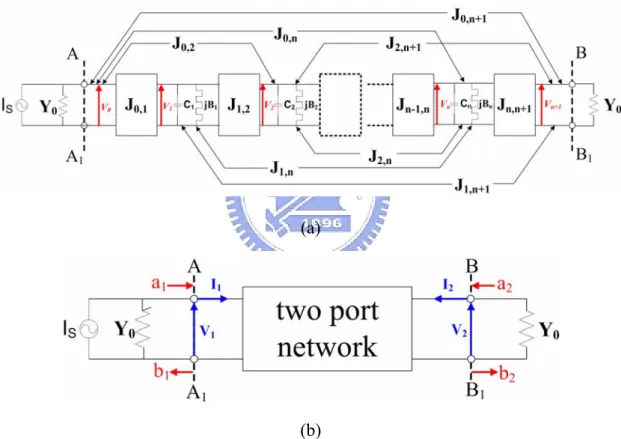
Figure 2-1 (a) Equivalent circuit of n-coupled resonators in low pass domain. (b) its network representation………...11
Figure 2-2 The coupling route of the example filter..…..………..16
Figure 2-3 Coupling route of a transversal filter..………..20
Figure 2-4 The flow of the optimization algorithm………27
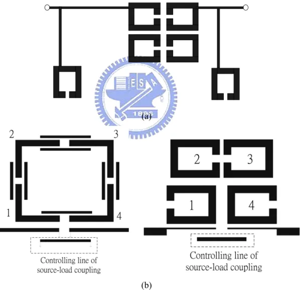
Figure 3-1 Microstrip implementation for (a) sixth-order quasi-elliptic filter with linear phase response using extracted-pole technique (b) proposed quadruplet filter with source-load coupling……….30
Figure 3-2 Coupling and routing scheme of symmetric cross-coupled quadruplet filter with source-load coupling (a) ideal case, (b) including the unwanted diagonal cross cuplings………32
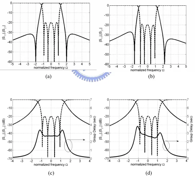
Figure 3-3 Quadruplet filters with (a) ideal quasi-elliptical response, (b) including unwanted cross coupling, (c) ideal flap group delay response, and (d) including unwanted cross coupling……….34
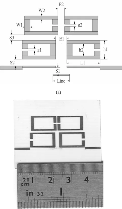
Figure 3-4 (a) quadruplet filter with the capacitive S/L coupling controlled by the controlling line (b) photograph of the fabricated filter with dimension (in mils) S1=4, S2=8, S3=41, E1=90, E2=20, W1=64, W2=30, h1=310, h2=250, g1=42, g2=26, Line=160……….40
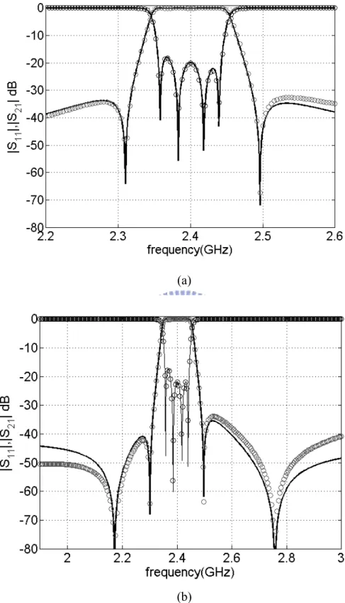
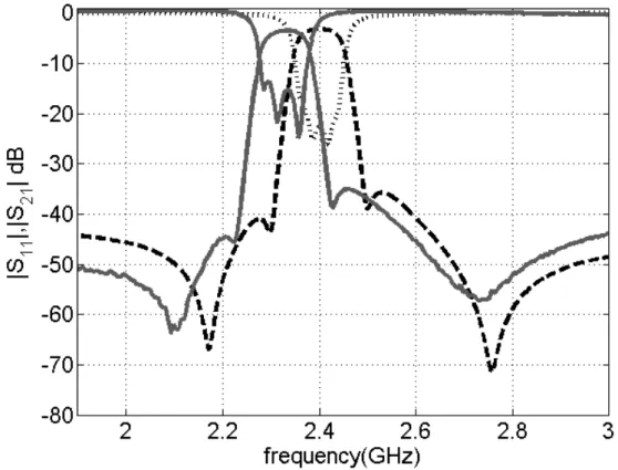
Figure 3-5 (a) response of quadruplet filter (b) response of quadruplet filter with controlling line of source-load coupling. Circle: EM simulated results; solid line: circuit model……….42
Figure 3-6 Experimental and circuit model results. Solid line: experimental results, dashed line: circuit model including loss term……….43
Figure 3-7 (a) quadruplet filter with the inductive S/L coupling controlled by the controlling line (b) photograph of the fabricated filter with dimension (in mils) d=20, Line=800, s=4, L3=575, L1=940, L2=770, L3=575, h1=340, h2=304…………44
Figure 3-8 Response of quadruplet filter with controlling line of source-load coupling. Circle: EM simulated results; solid line: circuit model………46 Figure 3-9 Experimental and circuit model results (a) return loss and insertion loss (b) group
delay. Solid line: experimental results, dashed Line: circuit model including loss term………..48 Figure 4-1 (a) The conventional parallel-coupled filter. (b) The modified filter. (c) The
coupling route of the modified filter………51 Figure 4-2 The layout of the fabricated filter (unit: mil). L1=354, L2=354, L3=354, L4=354,
S1=11, S2=35, W1=19, W2=21, K1=19, K2=20, T1=87, T2=39. The line with of coupling/shielding lines is 8mil………53 Figure 4-3 Simulated and measured responses. Solid line: measured results. Dashed lines:
EM simulated results………54 Figure 4-4 EM simulated results of three different cases. The dimensions of the simulated
filter are the same as these shown in Figure 4-2 except T2 is set to different values………55 Figure 5-1 Basic box-like coupling schemes for generalized Chebyshev-response filters
discussed in this paper. (a) doublet. (b) extended doublet (c) box-section. ( The gray area is realized by the proposed E-shaped resonator)……….57 Figure 5-2 A doublet filter (a) the proposed layout (gray area indicate the E-shaped resonator)
(b) the corresponding coupling scheme………58 Figure 5-3 Responses generated from the coupling matrix and from electrical network
shown in Fig. 2(a) with synthesis parameters………..63 Figure 5-4 A layout of extended-doublet filter and its corresponding coupling scheme. The
design is for flat group delay response………64 Figure 5-5 A layout of extended-doublet filter and corresponding coupling scheme. The
design is for skirt selectivity response………64 Figure 5-6 The extended-doublet filter with in-band return loss RL=20dB, normalized
transmission zeros at Ω=±2. (a) its coupling matrix (b) Responses of extended doublet filter and responses contributed by doublet only………66 Figure 5-7 A Box-section filter. (a) filter’s coupling scheme. (b) the proposed layout….68 Figure 5-8. A fourth order box-section filter: (a) its coupling matrix (b) the responses of the
box-section filter and ideal responses of the asynchronous tuned third-order hairpin-like filter calculated by M1 matrix………..70
Figure 5-9 Responses of the box-section filters. (a) Responses obtained by electrical parameters of design #1 in TableⅠ and its coupling matrix respectively. (b)
Responses obtained by electrical parameters of design #2 in Table Ⅰand its
coupling matrix respectively………73 Figure 5-10 Fabricated extended-doublet filter (a) layout(unit:mil) (b) simulated and
measured response………74 Figure 5-11 Fabricated box-section filter (a) layout (unit:mil) (b) simulated and measured
response. (c) the measured wideband response………75 Figure 5-12 A possible filter layout that can be modeled as a doublet configuration………..76 Figure 6-1 Canonical transversal array. (a) N—resonator transversal array including direct
source–load coupling MSL. (b) Equivalent circuit of the kth “low-pass resonator” in the transversal array………..80 Figure 6-2 The simulated and extracted results of the cross-coupled quadruplet filter under
Chapter 1 Introduction
Microwave filters are essential component in a microwave system. Thus, there are lots of literatures concerning with the designs and implementations of microwave filters applied in different wireless communication systems. Concerning with the development of the microwave filters, Ralph Levy et al. [1], [2] and Ian C. Hunter et al. [3] give a clear historical review of the development of microwave filters. Among these papers, different kinds of microwave filters are introduced and discussed, and important references are also given. Among different kinds of microwave filters, this dissertation would focus on the design and tuning of microwave filters which can be described by coupling matrices.
The design of microwave filters normally starts from the synthesis of a low-pass prototype network, regardless of the eventual physical realization in transmission line, waveguide, or other media. Low pass prototype networks are two-port network with an angular cutoff frequency of 1 rad/s and operating in a 1-Ω system. A typical prototype network is shown in Figure 1-1. The ladder network prototype in Figure 1-1(a) and (b) is an all-pole network with all its transmission zeros at infinity. The alternative network shown in Figure 1-1(c) and (d) are also used. The networks in Figure 1-1(c)(d) are very useful for the design of narrow band bandpass filter since it only use the series or shunt resonator. Besides, the network in Figure 1-1(c) or (d) can be described by a coupling matrix. To achieve more selective frequency response, like generalized Chebyshev response [1], finite transmission zeros in the complex plane have to be introduced, and the corresponding prototype circuit usually can be expressed by a cross-coupled network. Filters which can be modeled by a cross-coupled network are called cross-coupled filters. Cross couplings are usually generated by either putting resonant/non-resonant circuits or introducing couplings between nonadjacent resonators.
(a)
(b)
(c)
(d)
Figure 1-1. (a), (b) Lowpass prototype networks for “all-pole” filters. (c), (d) Alternative lowpass prototype networks using inverter.
1.1 Review of the Design of Cross-Coupled Resonator filters
The cross-coupled filters have been used since 1940’s [1]. An example is given following to explain the basic idea behind cross-coupled filters. A filter, utilizing the cross couplings between nonadjacent resonators, is shown in Figure 1-2. These cross couplings give a number of alternative paths which a signal may take between input and output ports. The multi-path effect causes transmission zeros to appear in the transfer function, which, depending on the phasing of the signals, may cause transmission zeros at finite frequencies or group delay flattening, or both simultaneously.
Figure 1-2. A cross-coupled resonator filter (clipped from Figure 9 in [1] )
Synthesis technique and implementation methods for the cross-coupled filters have been developed for couples of decades. Among those related works, the most significant development took place in the 1970’s in COMSAT by Atia and Williams [4]-[7]. The COMSAT work on elliptic function and linear-phase waveguide filters using dual-mode cavities with cross coupling was particular significant. The dual-mode cavity filters introduced by Atia and Williams have set the virtual standardization of these designs for satellite transponders. Actually, Atia and Williams have published a series of papers concerning on the synthesis, design, implementation, and tuning of the cross-coupled resonator filters. All those papers are well-written and introduce original concepts. It is highly recommended for one who is interested in the design of cross-coupled resonators filter to read the series of papers by Atia and Williams.
The most recent progress in the synthesis of cross-coupled filter is done by Richard Cameron. In 1999 and 2003, Richard Cameron published two papers focused on generalizing the synthesis technique for the cross-coupled resonator filter with the generalized Chebyshev function [8] [9]. With his work, a cross-coupled filter with N resonators can have at maximum N finite transmission zeros. Based on Cameron’s
work, many researchers have developed different methods to transfer the synthesized coupling matrixes into desired forms. The details of the related synthesis techniques will be discussed in Chapter 2.
The cross-coupling concept was originally used in the waveguide filters but not applied to the microstrip filters before 1990’s. But with the increasing power of computation of computers, the story was changed. Electromagnetic (EM) simulators are capable of simulating complex physical structures within a reasonable time now. Thus, it is feasible to get the S-parameters of the designed structure through the EM simulator instead of doing experiments. Hong and Lancaster took the advantage of the computer’s power to calculate the external quality factor and coupling coefficients, originally experimental method, to design the microstrip cross-coupled resonator filters [10], [11]. The related works done by Hong and Lancaster are clearly described in the book [12] written by them.
1.2 Motivation
The computer-aided diagnosis and tuning of cross-coupled resonator filters have been an active topic in the filter society for several decades. The main driving force to the art is the continuous demand on reducing the manufacturing cost and development time for various filters with different specifications. The core task in filter tuning is to diagnose the filter coupling status that corresponds to the current filter response. By comparing the desired circuit model parameters (i.e., coupling matrix) to the extracted ones, the tuning direction and magnitude can be decided.
Tuning is an essential process for optimizing filters’ responses in both the simulation stage and production line. On the simulation, even though a great variety of EM simulators are commercially available, it is generally impossible to optimize microwave filters on the basis of field simulators alone because the computer
simulation time for it is huge, especially for higher order filter with generalized Chebyshev response. Moreover, on the production line, fabrication of high performance filters is a constant trade-off between the manufacturing cost and the accuracy required in the process. In reality, the variation in raw material and manufacturing process leads the filters’ response deviate from the designed ones, which means post tuning is always required. The need of tuning on both EM simulation and fabrication urges filter designers to develop CAD tool to shorten the design period in recent decades.
In the design of cross-coupled resonator filter, especially for microstrip filter, the spurious couplings between resonators always exist. However, the method proposed by Hong and Lancaster only gives initial dimensions of microstrip cross-coupled filters [12]. The effect of spurious couplings between resonators and how to tune a filter to achieve a prescribed response were not mentioned. Thus, parameter extraction methods and tuning algorithm is needed to obtain the strength of spurious couplings and tune a filter.
1.3 Literatures Survey
The existing computer diagnosis techniques can be basically divided into two catalogues: by optimization technique and by analytical methods. There are pros and cons for the diagnosis techniques based on optimization methods and analytic formula, respectively. In the following, we will discuss them individually.
Basically, all the diagnosis and tuning procedures involving three basic elements 1. Filter synthesis
2. Curve fitting of a simulated or measured S-parameter, 3. Update of a filter’s physical dimensions.
These three basic elements in the procedure determine how good a procedure is. A simplified design flow of the filter tuning process is shown in Figure 1-3 to clarify the basic elements involved. The implementation of the flow shown in Figure 1-3 will be discussed in Chapter 2 in detail.
The methods based on nonlinear optimization are like that in [13]-[15] where different optimization strategies and schemes for parameter extraction are explored. In [13], the optimization technique is used to find a coupling matrix with the goal that the resulted response fitting well with the simulated response. However, there are many variables (coupling coefficients) involved in the optimization process, which makes the method only applicable for the cases where the order of filter is less than 6. The methods in [16], [17] are based on analytical method. Those methods extract the coupling matrix from the locations of system zeros and poles. The existing analytical models provide a recursive procedure to determine individual resonant frequencies and inter-resonator couplings. However, those analytical methods are only valid for highly restricted filter topologies. In addition, to get analytical formula for the calculation of the coupling matrix, one must derive different formula for different topologies, which is not easy even for an expert in this filed. Furthermore, the
S-parameters corresponding to an extracted coupling matrix usually can not so well fit the simulated or measured response as one can obtain by the optimization method because of the existence of dispersion effect. As we know, poles and zeros of a system determine the systems response. Moving one of the poles or zeros will change the response over all frequency. On the other hand, methods based on optimization can fit the simulated response better than the method based on analytical methods because sampling a lot of different frequency points over the interest band can average the dispersion effect. Filter specification S11(s) = F(s)/E(s) S21(s )= P(s)/E(s) Microwave filter S11(si), S21(si)
Mˆ
M
+-M
Δ
Circuital error: Physical dimension:y
Δ
0 x Correction:Δ
x
end δ < Δx No Yes synthesis updateFrom the above discussion, some observations are summarized. First, optimization technique should not be directly applied to obtain the coupling matrix as that in [13] since this approach limited the method only applicable to lower order filter. Second, reconstructing the coupling network from poles and zeros of system by analytical formula may not be accurate enough and be topology-limited.
In the procedure provided in [18], the Cauchy method is applied to obtain the approximated rational polynomials of reflection and transmission function,
) (
11 s
S andS21(s), which is suitable for filter synthesis. After getting the approximated rational polynomial of S11(s) andS21(s), a variety of synthesis techniques can be applied to get the coupling matrix. The synthesis technique used in [19] is based on optimization technique and can be applied to get a coupling matrix with arbitrary topology with the order smaller than 14. In practical, most cross-coupled resonators filters have the order smaller than 14. Thus, the procedure provided in [19] is highly recommended. Besides, there is no need to calibrate the reference plane when using the Cauchy method to get the approximated S11(s) andS21(s).
The formulation based on Cauchy method in [18] is only valid for lossless case. For lossy filters, the modified Cauchy methods are proposed in [20]. However, the method in [20] is incorrect in the sense that the generated rational polynomials,
) (
11 s
S andS21(s), are not suitable for the filter synthesis. The author in [21] indicated the theoretical error in [20] and proposed a modified formulation suitable for filters with low and moderate losses. It should be noted that even the formulation in [21] can not tell how lossy a filter is. So, how to model a lossy filter and extract related parameters is still a problem under investigate.
1.4 Contribution
The main contributions of this dissertation are described in the following.
First, an optimization procedure as shown in Figure 1-3 is developed in this dissertation. The optimization procedure is used to design all the circuits presented in this dissertation. It is also applied to investigate the effect of spurious couplings in the cross-coupled microstrip filters. Coupling matrices are extracted in the course to optimize the quadruplet filter with source-load coupling. With the developed optimization methods, quadruplet filters with various responses are designed, built, and tested.
Second, a microstrip cross-coupled filter with two independently controllable transmission zeros on upper stopband is presented. The initial filter structure is a conventional Chebyshev-response parallel-coupled filter that can be easily realized by the analytical method. The newly proposed coupling/shielding lines effectively control the cross and main couplings without changing the original filter layout. With this approach, designer can eliminate tedious segmentation method for the filter design.
Third, an E-shaped dual-mode resonator is proposed to implement coupling topologies such as doublet, extended doublet, and box-section in a unified approach. The doublet and box-section filter exhibit the zero-shifting properties which can not be achieved by trisection cross-coupled filters. The extended-doublet filter can generate two finite transmission zeros to improve selectivity or flatten in-band group delay. The correspondence between the E-shaped dual-mode resonator and a coupling matrix is established, which make it possible to design those filters in a systematical way.
Finally, the formulation which is applicable to extract the loss term and a coupling matrix simultaneously from a simulated or measured response is proposed.
With this method, no matter the device under test is lossy or lossless, one can extract the coupling matrix from the simulated or measured response.
1-5 Organization
This dissertation is mainly concentrated on the design and tuning of cross-coupled resonator filters, especially for the microstrip filters.
In Chapter 2, each step taken in the flow diagram of filter optimization in Figure 1-3 is discussed in detail. The model of the cross-coupled resonator filter in low pass domain is given. From the model, the relation between a coupling matrix and S-parameters is derived. Then, how to directly relate the position of finite transmission zeros to a given coupling matrix is given. Some simple topologies such as trisection, quadruplet, doublet, extended doublet, and box-section are taken as examples, and the equations relating the position of finite transmission zeros and coupling coefficients are given. In addition, a variety of synthesis methods are discussed, and the method for updating the physical dimension is given.
In Chapter 3, the quadruplet filters with source-load coupling are presented. The effect of spurious cross couplings between resonators is discussed. The parameter extraction method is applied to extract the coupling matrix corresponding to simulated response. The examples include the quadruplet filters designed for improving skirt selectivity and in-band group delay flatness.
In Chapter 4, a cascade trisection filter with source/load to multi-resonator couplings is proposed. The initial dimension of the filter is obtained from the conventional parallel coupled line filter. The filter exhibiting two finite transmission zeros which can be independently controlled to improve the selectivity.
In Chapter 5, generalized Chebyshev microstrip filters with box-like coupling schemes are presented. The box-like portion of the coupling schemes is implemented by an E-shaped resonator. Synthesis and realization procedures are described in detail.
In Chapter 6, a parameter extraction method based on vector fitting formulation is proposed to identify the unload quality factor of resonators and coupling matrix of a filter from the simulated/measured response simultaneously.
Chapter 2 Design and Optimization of Microwave Filter
Based on Coupling Matrix
In this chapter, the design flow of cross-coupled resonator filters is given and discussed in detail. To facilitate the discussion, the cross-coupled resonators network is analyzed in the normalized frequency domain at first. The relation between the normalized network parameters and S-parameters is derived. How to obtain the position of finite transmission zeros from coupling topologies is also given. With the necessary background, each step shown in Figure 1-3 is given.
(a)
(b)
Figure 2-1 (a) Equivalent circuit of n-coupled resonators in low pass domain. (b) Its network representation.
2.1 Filter Model in the Normalized Domain
A prototype filter of degree n in the lowpass domain is shown in Figure 2-1 (a). The prototype filter consists of frequency independent impedance inverters Jijs, capacitors Cis and susceptances Bis. The values of all the capacitors and the
terminated admittances Y0 are set equal to one. The capacitors in the low-pass domain correspond to the resonators in the bandpass domain. Thus, the frequency invariant susceptances Bis represent the frequency shift of resonators in the bandpass domain. The values of Bis are zero for the synchronously tuned filters and nonzero for the asynchronously tuned filters.
According to the current law, which is one of the Kirchhoff’s two circuit laws and states the algebraic sum of the currents leaving a node in a network is zero, with a driving or external current of I , the node equations for the circuit of Figure 2-1(a) s
are 1 ) 2 ( 1 ) 2 ( 1 1 0 ) 2 ( ) 2 ( 0 1 , 1 , 1 1 , 0 1 , 2 , 1 2 , 0 1 , 1 2 , 1 1 1 , 0 1 , 0 2 , 0 1 , 0 0 0 0 0 × + × + + + × + + + + + + + ⎥ ⎥ ⎥ ⎥ ⎥ ⎥ ⎦ ⎤ ⎢ ⎢ ⎢ ⎢ ⎢ ⎢ ⎣ ⎡ = ⎥ ⎥ ⎥ ⎥ ⎥ ⎥ ⎦ ⎤ ⎢ ⎢ ⎢ ⎢ ⎢ ⎢ ⎣ ⎡ ⎥ ⎥ ⎥ ⎥ ⎥ ⎥ ⎦ ⎤ ⎢ ⎢ ⎢ ⎢ ⎢ ⎢ ⎣ ⎡ + Ω + Ω n s n n n n n n n n n n n n n n I V V V V Y jJ jJ jJ jJ jB j jJ jJ jJ jJ jB j jJ jJ jJ jJ Y M M L M M M O L L (2-1)
where Ω is the normalized frequency.
To derive the two-port S-parameters of a coupled-resonator filter, the circuit of Figure 2-1(a) is represented by a two-port network of Figure 2-1(b). Comparing Figure 2-1(a) and Figure 2-1(b), we can find that V1=V0, V2=Vn+1, and I1=Is-Y0V0.
And 2 1 s I a = , 2 2 0 1 s i V b = − 0 2 = a , b2 =Vn+1 Thus, s a I V a b S 0 0 1 1 11 2 1 2 + − = = = (2-2) s n a I V a b S 1 0 1 2 21 2 2 + = = = (2-3)
From equation (2-1), we can obtain
[ ]
1 1 , 1 0 = Y − I V s (2-4)[ ]
1 1 ), 2 ( 1 − + + = n s n Y I V (2-5) Take (2-4) into (2-2), we can obtain1 1 , 1 11 1 2[ ] − + − = Y S (2-6) Take (2-5) into (2-3), we can obtain
1 1 , 2 21 2[ ] − + = Y n S (2-7)
In the literatures, the matrix
⎥ ⎥ ⎥ ⎥ ⎥ ⎥ ⎦ ⎤ ⎢ ⎢ ⎢ ⎢ ⎢ ⎢ ⎣ ⎡ + + + + + + 0 0 1 , 1 , 1 1 , 0 1 , 2 , 1 2 , 0 1 , 1 2 , 1 1 1 , 0 1 , 0 2 , 0 1 , 0 n n n n n n n n n J J J J B J J J J B J J J J L M M M O L L is called the
normalized coupling matrix and denoted as matrix [M].
⎥ ⎥ ⎥ ⎥ ⎥ ⎥ ⎦ ⎤ ⎢ ⎢ ⎢ ⎢ ⎢ ⎢ ⎣ ⎡ = 0 0 ] [ 1 12 2 1 12 11 1 2 1 nL L SL nL nn S L S SL S S M M M M M M M M M M M M M M M L M M M O L L
Where Mij =Ji,j , Mii =Bi. To translate the equation (2-6) and (2-7) to the expressions in the literatures, let
(
[ ] [ ] [ ])
[ ] ] [ ] [ ] [ ] [Y =s I + j M + G = j Ω U 0+ M − j G = j A , where ][A]=Ω[U]0+[M]− j[G , ( 2)( 2) 0][U ∈Rn+ ×n+ is identical to the identity matrix, except for the element [U0]11=[U0]n+ n2, +2 =0, and [G]∈R(n+2)×(n+2) is also a diagonal matrix, [G]=diag{1,0,L,0,1}. The equations (2-6) and (2-7) can be rewritten as
1 1 , 1 11 1 2 [ ] − − − = j A S (2-8) S21=−2 j
[ ]
A−(n1+2),1 (2-9) Similarly, we can derive1 2 , 2 22 1 2 [ ] − + + − − = j A n n S (2-10)
The equations (2-8), (2-9) and (2-10) directly related the normalized coupling matrix to the S-parameters.
2.2 The Position of Finite Transmission Zeros
From the equations (2-8) and (2-9), we can express S11 and S22 as a rational functions, ) ( ) ( ) ( 11 Ω Ω = Ω E F S (2-10) ) ( ) ( ) ( 21 Ω Ω = Ω E P S (2-11) Obviously, the finite transmission zeros are the roots of the equation
P(Ω)=0 (2-12)
Solving the equation (2-12) can help us understand the dependence between the coupling coefficients and finite transmission zeros, which help us get more insight to control the finite transmission zeros. To illustrate that, let us take an example with the coupling matrix M1 ⎥ ⎥ ⎥ ⎥ ⎥ ⎥ ⎥ ⎥ ⎦ ⎤ ⎢ ⎢ ⎢ ⎢ ⎢ ⎢ ⎢ ⎢ ⎣ ⎡ = 0 0 0 0 0 0 0 0 0 0 0 0 0 0 0 0 0 0 0 0 0 0 0 0 4 4 34 14 34 23 23 12 14 12 1 1 1 L L S S M M M M M M M M M M M M M (2-13)
The topology of M1 is known as cross-coupled quadruplet and the graphical representation of it is drawn in Figure 2-2. This kind of graphical representation has
been widely used in literatures recently.
Figure 2-2 the coupling route of the example filter
By solvingP(Ω)=0, we can find the roots can be expressed as 14 34 23 12 2 23 2 M M M M M Ω = − (2-14)
The cross-coupled quadruplet filter is a perturbation version of the original direct-coupled Chebyshev filter. Thus, compared to the values of M12, M23 and M34, the value of M14 is relatively small. That is
14 34 23 12 2 23 M M M M M < .
For the design where the shape skirt selectivity is required on both side of the pass band, the finite transmission zeros should be put on the real frequency axis, which means Ω2 >0. On the other hand, for the group delay flattening, the finite transmission zeros should be put on the imaginary frequency axis, which means
0 2 <
Ω . From the equation (2-14), we can tell that if M12M23M34M14 <0 , thenΩ2 >0 and if 0 14 34 23 12M M M > M , then Ω2 <0.
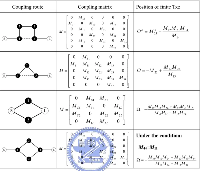
The coupling topologies: quadruplet, trisection, doublet and box-section, are given in Table 2-1. The corresponding position of finite transmission zeros of these topologies are given in Table 2-1 as well.
Coupling route Coupling matrix Position of finite Txz ⎥ ⎥ ⎥ ⎥ ⎥ ⎥ ⎥ ⎥ ⎦ ⎤ ⎢ ⎢ ⎢ ⎢ ⎢ ⎢ ⎢ ⎢ ⎣ ⎡ = 0 0 0 0 0 0 0 0 0 0 0 0 0 0 0 0 0 0 0 0 0 0 0 0 4 4 34 14 34 23 23 12 14 12 1 1 L L S S M M M M M M M M M M M M M 14 34 23 12 2 23 2 M M M M M Ω = − ⎥ ⎥ ⎥ ⎥ ⎥ ⎥ ⎦ ⎤ ⎢ ⎢ ⎢ ⎢ ⎢ ⎢ ⎣ ⎡ = 0 0 0 0 0 0 0 0 0 0 0 0 3 3 33 23 13 23 22 12 13 12 11 1 1 L L S S M M M M M M M M M M M M M M 13 23 12 22 M M M M Ω=− + ⎥ ⎥ ⎥ ⎥ ⎦ ⎤ ⎢ ⎢ ⎢ ⎢ ⎣ ⎡ = 0 0 0 0 0 0 2 1 2 22 2 1 11 1 2 1 L L L S L S S S M M M M M M M M M M M L s L s L s L s M M M M M M M M M M 2 2 1 1 1 1 22 2 2 11 + + − = Ω ⎥ ⎥ ⎥ ⎥ ⎥ ⎥ ⎥ ⎥ ⎦ ⎤ ⎢ ⎢ ⎢ ⎢ ⎢ ⎢ ⎢ ⎢ ⎣ ⎡ = 0 0 0 0 0 0 0 0 0 0 0 0 0 0 0 0 0 0 0 0 4 4 44 34 24 34 33 13 24 22 12 13 12 11 1 1 L L S S M M M M M M M M M M M M M M M M M
Under the condition:
M44=M11 34 13 24 12 34 13 22 24 12 33 M M M M M M M M M M + + − = Ω
Table 2-1. Coupling topologies and the position of their corresponding finite transmission zeros
2.3 Synthesis Methods for Cross-Coupled Filters
Filters may be classified into categories in several ways, one being into different classes of response functions, defined in terms of the location of poles of the insertion-loss function and of the zeros within the passband. The zeros are usually spaced throughout the passband to give a Chebyshev response since this is far more optimum and superior to the maximally flat or Butterworth response, which is rarely used. As far as the poles are concerned, the most common type of filter response has these located all at dc and infinity and is often described as an all-pole Chebyshev
filter. When one or more poles are introduced into the stopband at finite frequencies, a filter is called a generalized Chebyshev filter or a pseudo-elliptic filter.
From the discussion in section 2.1 and 2.2, we know cross-coupled filters exhibit finite transmission zeros (attenuation poles), which means the responses of cross-coupled filters may correspond to the generalized Chebyshev response. In fact, how to generate the S11(s) and S21(s) corresponding to the generalized Chebyshev function and find the corresponding coupling matrix are well-established [4]-[9]. The method about how to generate rational functions, S11(s) and S21(s), corresponding to the generalized Chebyshev response are given in [8]. The generated S11(s)and
) (
21 s
S are in the form
) ( ) ( ) ( 11 s E s F s S = (2-15) ) ( ) ( ) ( 21 s E s P s S = (2-16)
Synthesis methods about how to get the coupling matrix corresponding to the specified response in (2-15) and (2-16) may be divided into three categories.
1. Direct optimization
In 1998, Atia first proposed that with suitable cost function defined with positions of poles and zeros of a transfer function, we can set coupling coefficients of a filter as variables and apply the optimization method to get a coupling matrix [22] corresponding to that transfer function. Later, Amari extended Atia’s work to include the source-load coupling [23]. The drawback of this kinds of method is that they are only effective for the filter with order smaller than 6. On the other hand, this kind of method is easy to follow and implement in a circuit simulator, like ADS.
2. Analytical method
The analytical method for the synthesis of cross-coupled filters was originally presented by Atia and Williams in [5]. Recently, Cameron has extended the analytical method to generate a generic matrix corresponding to a generalized Chebyshev response [8]. The generic matrix is n×n matrix having the form
⎥
⎥
⎥
⎥
⎥
⎥
⎦
⎤
⎢
⎢
⎢
⎢
⎢
⎢
⎣
⎡
=
nn n n n n n nM
M
M
M
M
M
M
M
M
M
M
M
M
M
M
M
M
L
M
O
M
M
M
L
L
L
3 2 1 3 33 32 31 2 23 22 21 1 13 12 11where Mij=Mji. The external coupling between the first resonator to source or last resonator to load is not shown in the matrix but expressed by two additional parameters R1 and R2. Since the source-load coupling is not included in the formulation, this kind of synthesis method can only apply for nth order filter with maximum of (n-2) finite transmission zeros. Besides, the matrix in generic form has to be further reduced since the coupling route is too complicated to achieve practically.
In 2003, Cameron further generalized the synthesis technique to cover the cases where source-load and source/load to multi-resonator couplings are involved. Follow the analytical formula in [9], we can get a transversal matrix with size(n+2)×(n+2). To distinguish coupling matrix with size (n+2)×(n+2) to that with size n×n, we usually call a coupling matrix with size (n+2)×(n+2)an extended coupling matrix. A transversal coupling matrix is an extended coupling matrix with the following form
⎥
⎥
⎥
⎥
⎥
⎥
⎦
⎤
⎢
⎢
⎢
⎢
⎢
⎢
⎣
⎡
=
0
0
0
0
2 2 1 11 1 2 1 Ln L LS nL nn S L S SL S SM
M
M
M
M
M
M
M
M
M
M
M
M
L
M
M
M
M
L
O
L
L
The corresponding coupling route of the transversal topology is shown in Figure 2-3
Figure 2-3. Coupling route of a transversal filter
The transversal matrix need to be further transformed into other coupling routes since the coupling route in transversal configuration is too sensitive to realize when the order of filter exceeds 2 [24]. From the above discussion, we know that both the generic and transversal coupling matrix are impractical. Thus, how to annihilate some couplings to make a coupling matrix simpler and keep the same electrical performance is important.
The technique of annihilating some specific couplings in a coupling matrix is called matrix reduction. The method for matrix reduction has been studied for several
decades. In principle, we can apply a sequence of similarity transforms to a generic or transversal matrix until more convenient form with a minimal number of couplings is obtained [5], [8], [9]. The similar transformation would not change the eigenvalues and eigenvectors of the coupling matrix, which means a transferred coupling matrix would exhibit the same response as the original coupling matrix. There are only a few patterns of coupling matrix can be achieved in a predetermined way, and most of them are proposed by Cameron [8], [9]. The analytical method is very powerful in the sense that the order of filter is not limited. However, how to transfer the generic or transversal coupling matrix into suitable topologies is not easy at all.
In view of the difficult of determine the rotation angles of the sequence of similar transformation, optimization method is introduced [25]. The method in [25] is reported to be effective for filter with order below 12. Another power optimization method based on the conservation of eigenvalues is proposed in [19], which is effective for filter with order under 14 and taken in this dissertation.
2.4 Obtaining a Initial Design for a Microwave Filter
With the information of a coupling matrix, we may obtain the initial dimension of microwave filters. A widely applied method to get the initial dimension of a filter is the segmentation method. In the segmentation method, the coupling strength between resonators is tested pair by pair to obtain the approximated coupling strength. The external coupling, the coupling between the first/last resonator to the source/load, is calculated by excluding other resonators. The detail of segmentation method formulated in low-pass domain is provided in Chapter 4 in the book [26]. In addition, formulation in the bandpass domain is given in the chapter 8 in the book [12]. In principle, it is better to do the calculation in the low-pass domain since the formulas are much simpler.
2.5 Tuning Procedures
The tuning of a microwave filter consists of two major steps. First, extract the coupling matrix from the simulated or measured response. Second, decide how to adjust the geometrical dimension of the filter under test by comparing the difference between extracted coupling matrix and the wanted coupling matrix.
A. parameter extraction
As we discussed in section 2.2 and 2.3, it is feasible to express the S-parameters of a filter as a rational polynomials in normalized frequency domain. So, if we can identify the S-parameters in rational polynomials in normalized frequency domain from the simulated or measured response, we can use the synthesis technique to obtain a coupling matrix. For S-parameter identification, an effective method, called Cauchy method, is proposed. The detail of the method is given in [18]. Here, we just give a brief review of the Cauchy method and point out some important characteristics of it.
The purpose of Cauchy method is to obtain the approximated rational polynomials of S~11(s) and S~21(s) in the following form
∑
∑
= = = = n k k k n k k k s b s a s E s F s S 0 0 ) 1 ( 11 ) ( ~( ) ~ ) ( ~ (2-17)∑
∑
= = = = n k k k n k k k s b s a s E s P s S z 0 0 ) 2 ( 21 ) ( ~( ) ~ ) ( ~ (2-18)In the Eq. (2-17) (2-18), n is the order of filter and nz is the number of finite transmission zeros. Note that the S~11(s) and S~21(s) have common denominator. Instead of directly fitting the simulated or measured data into the rational polynomial
) ( ~
11 s
) ( ~ / ) ( ~ ) (s S11 s S21 s
K = . In this step, one can obtain the F~(s) and P~(s). The second step is to reconstruct the polynomial E~(s) by the Feldtkeller’s equation:
F~(s)F~*(−s)+P~(s)P~*(−s)=E~(s)E~*(−s) (2-19) Note that there is no need to calibrate the reference plane before applying the Cauchy method, which makes the Cauchy method a perfect CAD tool. After obtaining the approximated rational polynomials in (2-17) and (2-18), the synthesis method given in section 2.3 can be directly applied to obtain the coupling matrix M~ . The M~ represents the equivalent electrical parameters of the filter corresponding to the present geometrical dimensions.
B. Update the geometrical parameters
The cross-coupled network shown in Figure 2-1 can be treated as a surrogate model. The status of the surrogate model is represented by a coupling matrix. The object of filter diagnosis is to decide how to adjust the geometrical dimension of a filter by comparing the extracted coupling matrix M~ to the object coupling matrix
obj
M , where Mobj correspond to the desired response.
In a coupling matrix, only the nonzero elements are significant since they represent either the coupling coefficients or the shifting of resonant frequencies. To facilitate the discussion, we collect those nonzero elements to form a vector y and collect the geometrical parameters of the filter to form a vector x . The relation
between vector y and vector x can be denote as y= f(x). The object surrogate parameters can be denoted as yobj. The present geometrical parameters of the filter can be donated as x0 and its corresponding significant surrogate parameters can be donated as y0. The goal of optimization is to find an optimal geometrical parameter
opt
x to let the corresponding yopt approach yobj So, updating the vector x from
0
x to xopt is the core of the optimization. The update method used in [13] is taken in this dissertation and outlined in the following.
Before the surrogate model can be optimized, the sensitivities of the parameters with respect to the geometrical parameters must be determined. This is done by using finite difference approximation as described in the following four steps:
1. Calculate S-parameter of the filter structure in basis (non-ideal) position using the field solver and extract the characteristic parameters : basis
ii basis
ij M
M~ , ~
2. Change first geometry parameter to x1+Δx1, and repeat step 1ÎM~ijx1+Δx,M~iix1+Δx
3. Repeat step2 for all other geometry parameters x2,x3,....,xn
The above information is to construct the first order Taylor expansion with respect to the initial design (the initial design must be near the solution, otherwise the convergence is not guaranteed).
4. The surrogate model can be approximated as
k n k k basis ij x x ij n basis ij k n k k k k basis ij x x ij n basis ij n n surrogate ij d x M M x x x M d x x x M M x x x M d x d x d x M k k k k
∑
∑
= Δ + = Δ + Δ − + = − Δ + − + = + + + 1 2 1 1 2 1 2 2 1 1 ) ~ ~ ( ) ,..., , ( ~ ) ) ( ~ ~ ( ) ,..., , ( ~ ) ,...., , ( ) ,..., , ( 1 2 n basis ij x x x M , and ) ) ( ( k k k basis ij x x ij x x x M M k k − Δ + − Δ +are determined in the first three steps. The object of optimization is to determine the set {d1,d2,...dn} which minimize the difference between coupling matrix of surrogate model and object coupling matrix get from standard filter synthesis. The cost function is defined as
∑∑
∑
− + + + + − + + + = j i obj ij n n surrogate ij i obj ii n n surrogate ii n M d x d x d x M M d x d x d x M d d d U 2 2 2 1 1 2 2 2 1 1 2 1 ) ) ,...., , ( ( ) ) ,...., , ( ( ) ,..., , (The termination condition can be set by the value of cost function U(d1,d2,...,dn) or by the value of dr 2, where dr=(d1,d2,L,dn). If the updated geometric parameters do not exhibit the desired response, repeat the step1 to step 4 until the termination condition is achieved. It usually takes several times for the optimization since in most case the parameters of surrogate model are not a linear function of the geometry parameters. However, this method is attractive since the step can easily be followed in practice. Besides, testing the sensitivity is crucial since it not only give the information of how to update the filter but also give a measure of how sensitive a filter is.
2.6 The Optimization Flow of Cross-Coupled Microwave Filters
In this section, the step by step optimization algorithm is given. The flow of the optimization algorithm is shown in Figure 2-4. Each step is numbered.
1. Give a specification.
2. Generation of the ideal characteristic polynomials,F(s),P(s),E(s)which satisfy specifications.
3. Synthesis of the ideal coupling matrix M which would be the object matrix we want to achieve in the optimization process.
The methods for the first three steps are given in section 2.3.
4. Computation of the initial dimensions of the microwave filter from the information of the ideal coupling matrix by segmentation method. Detail is given
in section 2.4.
5. Simulate the circuit in an EM simulator. Then, acquire N samples points of S-parameters, )S11(si S21(si) from the simulated response to reconstruct the rational model, S~11(s) and S~21(s), by Cauchy method. The detail is given in section 2.5.
6. Synthesize the coupling matrix corresponding to the rational functions S~11(s) and S~21(s). The obtained coupling matrix is M~. The synthesis technique is the same as that used in step 3.
7. Calculate the difference between the object coupling matrix Mobjand extracted coupling matrix M~ . ΔM =M~−Mobj.
8. Do the sensitivity test
9. Generate the correction vector,dr, for the geometric parameters of the filter. The methods for Step 7 to step 9 are given in section 2.5.
10. If the change of the geometric dimension is small enough (depending on the limitation of the fabrication), then stop the optimization procedure. Otherwise, change the geometric dimension to be x0 +Δx and repeat step 4 to step 10.
2.7 Limitations of the Proposed Design Flow
The diagnosis and tuning process presented in this Chapter is only true for filters which can be described by the cross-coupled network shown in Figure 2-1(a). Thus, the correspondence between a physical layout and a cross-coupled prototype network, served as surrogate model, must be tested at first. This kind of test can be achieved in the process of sensitivity test. By observing the shift of the resonant frequencies or variation of coupling coefficients as the physical dimension is changed, we can tell whether the correspondence between the physical layout and surrogate model exists.
The surrogate model used in this dissertation can only apply for narrow band filters. The maximum fractional bandwidth may range from 10% to 40% depending on the type of resonators and coupling methods. The diagnosis and tuning process is not a “black box” process, which means knowing more about the design process would help do the parameter extraction and diagnosis. For example, when doing the design, the formula for lowpass to bandpass transformation may differ from design to design. When doing the diagnosis, we must map the frequency response from bandpass domain to lowpass domain by the bandpass to lowpass transformation. Definitely, the bandpass to lowpass transformation is the reverse operation of the lowpass to bandpass transformation used in the design. Thus, knowing the lowpass to bandpass transformation used in the design is important for the process of filter diagnosis.
Chapter 3 Cross-Coupled Filters with Source-Load Coupling
In this chapter, quadruplet microstrip filters with source-load coupling are proposed to achieve similar skirt selectivity and/or in-band flat group delay as that of a sixth-order canonical form or an extracted pole microstrip filter. Diagnosis method of unwanted effects such as asynchronous resonant frequencies and unwanted couplings, which often occurs in microstrip’s open environment, is described in detail. A systematic design flow to implement a quadruplet microstrip source-load coupled filter with proper filter response is also provided. Two trial filters exhibited quasi-elliptical and flat group delay response are designed and fabricated. Both theoretical and experimental results are presented.
3.1 Introduction
High performance microstrip filters with high selectivity and linear in-band phase response has been studied over the last two decades [12]. Additional cross coupling between nonadjacent resonators are often used to generate finite transmission zeros for high selectivity, or linear phase. Naturally, the topology of the coupling network determines the number of finite transmission zeros, whereas the relative signs and magnitudes of the different coupling coefficients control the positions of finite transmission zeros. Some well-known topologies such as canonical form, cascade quadruplet (CQ), cascade trisection (CT) [12], and extracted-pole [27] have been successfully realized using microstrip. For instance, Jokela [28] has shown that sixth-order canonical form filter can achieve both high selectivity and linear phase, which is attractive when comparing the passband insertion loss with the CQ filter. In the CQ configuration, a minimal of eighth order is required to generate the real-frequency transmission zeros pair for selectivity, and real-axis transmission zeros
pair for linear phase. An eighth-order CQ filter introduces more insertion loss than that of a sixth-order canonical form filter, but it gains the independent control of transmission zeros where the design and tuning becomes easy. However, there are some disadvantages attached to the canonical structure as mentioned in [27]. Besides, according to Jokela’s paper [28], the in-band flat group delay and skirt selectivity can be obtained simultaneously but a requirement of M25=0 should hold for easy implementation. This requirement simplifies the coupling routine but greatly constrains the freedom of choice of filter response.
(a)
(b)
Figure 3-1 Microstrip implementation for (a) sixth-order quasi-elliptic filter with linear phase response using extracted-pole technique (b) proposed quadruplet filter with source-load coupling.
To avoid the disadvantage of the canonical form filter, Yeo et al. [27] proposed the extracted-pole microstrip filter as shown in Figure 3-1(a) where the concept is originally used in a waveguide filter. The extracted-pole filter depicts better control of finite transmission zeros than that of canonical form filter, but it is relatively large due to the need of phase shifters. Here, we propose the fourth-order filter with source-load coupling, as shown in Figure 3-1(b), to generate two pairs of transmission zeros as sixth-order canonical form or eighth-order CQ filter does. The synthesis methods of the symmetric resonator filters with source-load coupling are well documented in literatures [23, 29]. Coupling diagram of the symmetric fourth-order filter with source-load coupling is shown in Figure 3-2(a). However, in realistic implementation of microstrip filter, the unwanted cross couplings always exist and lead the coupling route becomes complicated as shown in Figure 3-2(b). To identify all parameters corresponding to unwanted cross couplings, frequency alignment, and source-load coupling, powerful CAD tools are needed. Recently, an elegant diagnosis method is proposed to help designing of symmetric coupled-resonator filters [17]. However, the method in [17] has not taken the source-load coupling into account. In this chapter, we propose a diagnosis scheme, which is applicable to arbitrary topologies with or without source-load coupling.
This chapter is organized as follows. In section 3.2, the phenomenon of asymmetric responses of quadruplet filter is discussed and design guidelines are provided. In section 3.3, the CAD method is introduced to extract the coupling matrix with prescribed topologies. In section 3.4, the diagnosis method is applied to designing the proposed filter. Both theoretical and experimental results are presented for comparison.
(a) (b)
Figure 3-2 Coupling and routing scheme of symmetric cross-coupled quadruplet filter with source-load coupling (a) ideal case, (b) including the unwanted diagonal cross couplings.
3.2 Asymmetric Frequency Responses
The fourth order cross-coupled quadruplet filter is the well-known building block for generating a pair of finite transmission zeros, which can improve skirt selectivity or in-band group delay flatness. The conventional coupling diagram of quadruplet filter is similar to Figure 3-2(a) except source-load coupling is excluded. The explicit relation between the finite transmission zeros and the coupling coefficients of it can be expressed in lowpass domain as follows
14 34 23 12 2 23 2 M M M M M Ω = − (3-1)
In Eq. (3-1),Ω is the normalized frequency and Mij are the coupling coefficients in lowpass prototype. The relation between Ω and actual frequency f is
) / / )( / (f0 Δf f f0 − f0 f =
Ω , where f0 is the center frequency of the filter, and Δ f
is the bandwidth of the filter. For improving the skirt selectivity of the filter, the finite transmission zeros are put in real frequency axis and the relation M12 M23 M34 M14 < 0 must be satisfied. On the other hand, to generate the imaginary frequency transmission zeros for in-band group delay flatness, M12 M23 M34 M14 > 0 must hold.
However, the unwanted diagonal cross couplings always exist in the microstrip cross-coupled filter due to microstrip’s open environment. Both unwanted diagonal cross couplings and asynchronous resonant frequencies of resonators would distort the ideal symmetric response of the reflection coefficient |S11| and transmission coefficient |S21|. In [17, 30], the authors have shown how to extract the unwanted diagonal cross couplings and to adjust the resonant frequencies of resonators to compensate the distortion of return loss for a skirt selectivity filter. However, in the case of flat group delay filter we find that the unwanted cross couplings seriously degrade the flatness of in-band group delay and should be suppressed to a negligible level. Figure 3-3 shows some examples to demonstrate the phenomena. In Figure 3-3(a), an ideal response of the synchronous-tuned quadruplet filter with symmetric finite transmission zeros at Ω=±2 is shown. If the values of unwanted cross couplings M13 and M24 are equal to –0.06, the frequency response after adjusting the resonant frequencies is shown in Figure 3-3(b). It can be observed that the transmission zeros drift slightly and the height of |S21| bumps tilts. In many practical applications this change of |S21| is acceptable. However, in the case of flat group delay filter as shown in Figure 3-3(c), the finite transmission zeros are located at
55 . 1 j ± =
Ω . Set M13=M24=-0.06, which is similar to the previous case, and adjust the resonant frequency to optimize the in-band return loss, we would get the results as shown in Figure 3-3(d). It is obvious that the response of |S21| has negligible change but the in-band group delay tilts seriously. In most of linear phase filter applications this tilting of group delay is not allowed.
From the above discussion, some observations are summarized as follows. First, higher order symmetric filters in folded form are hard to design since tuning of resonant frequencies is needed for compensating the in-band return loss distortion. Besides, controlling more than one pair of finite transmission zeros and keep the
return loss good is even more difficult. On the contrary, the source-load coupling has extremely small contribution to the passband response and is much easier to implement extra pair of transmission zeros. In other words, we can control the additional pair of finite transmission zeros and keep the original finite transmission zeros nearly unchanged by merely adjusting source-load coupling without fine-tuning other portion of the filter. Second, the unwanted cross coupling is surprisingly harmful to the performance of in-band flap group delay response. The only way to implement a good in-band flap group delay filter is to avoid the unwanted cross coupling.
(a) (b)
(c) (d)
Figure 3-3. Quadruplet filters with (a) ideal quasi-elliptical response, (b) including unwanted cross coupling, (c) ideal flap group delay response, and (d) including unwanted cross coupling.