Many human exposure and epidemiologic studies have investigated associations between pollutant exposure and disease risk and their potential consequences (Aickin 2002; Chen et al. 2004). For studies on ambient air pol-lutants, because of the substantial cost and logistic constraints, personal exposure moni-toring can be used only for a small number of study participants, thus resulting in low statis-tical power to detect small effects (Ozkaynak et al. 1996). Most air pollution epidemio-logic investigations use individual health data sets at nationwide or regional scales to assess the subtle risks of pollution exposure. In these cases, ambient air-quality monitor-ing networks, such as the Air Quality System (AQS) operated by the U.S. Environmental Protection Agency (EPA), constitute impor-tant and useful environmental data sources concerning the acute and chronic effects of ambient pollutants (U.S. EPA 2002).
Although these environmental monitor-ing data sources provide useful information to estimate human exposure across space and time, environmental epidemiologists and exposure scientists still face several practical
and methodologic challenges in analyzing and modeling the environmental data (Li et al. 2008; Mutshinda et al. 2008).
One challenge is the geographic coverage of the region of interest. Ideally, if the pollu-tion-monitoring stations are located near the residences of the study participants, a partici-pant’s exposure could be easily estimated from neighboring pollutant observations (Maxwell and Kastenberg 1999; Wu et al. 2004). Unfortunately, the AQS monitoring network is relatively scarce compared with the number and geographic distribution of participants considered in large epidemiologic studies, and the geographic locations with direct ambi-ent observations are often at large distances from the places where the study participants reside. To address this issue while assessing individual-level exposures, the geocoding of the subjects’ residential addresses is usually combined with some form of interpolation of likely pollution levels between monitoring locations. Spatial interpolation techniques can be used to estimate large-region pollu tant exposures, including deterministic inverse distance schemes (Michelozzi et al. 2002),
Monte Carlo methods (Kentel and Aral 2005), and kriging techniques (Christakos and Thesing 1993; Liao et al. 2006; Rushton et al. 1996). Kriging techniques, in particular, have been applied with increasing frequency in large-scale epidemiologic studies, including long-term exposure assessment (Brauer et al. 2003; Hoek et al. 2001). However, because of their inherent constraints (estimator linearity, probabilistic normality, and limited interpre-tive features that cannot consider highly rel-evant qualitative knowledge), the mainstream kriging techniques do not always address suc-cessfully important human exposure issues, including the integration of composite space– time dependencies and the assimilation of soft (uncertain) information sources that are prevalent in most human exposure studies.
The second issue relates to the limited sampling frequency of environmental moni-toring networks. For example, the current AQS monitoring database includes particu-late matter (PM) data sampled at 1-, 2-, 3-, 6-, and 9-day cycles (note that most data are sampled at a 6-day cycle). As a result, even if the residences of the study participants are very close to ambient air monitoring stations, some considerable pollution events likely occur during times when the local monitor-ing stations are not operatmonitor-ing. To address this issue, which is often a significant concern to time-series analyses and epidemiologic panel studies of acute health effects, a smoothing technique is often applied to estimate ambi-ent air pollutant levels that were missing during the times of interest (Conceicao et al. 2001; Sagiv et al. 2005). Nevertheless, nei-ther spatial nor temporal analyses have fully accounted for and taken advantage of the exposure variability generated in a composite space–time dependence domain. Remarkably, the temporal domain of AQS air pollution monitoring is considerably more extensive Address correspondence to Hwa-Lung Yu, No. 1 Roosevelt Rd., Sec. 4, Taipei, 10617, Taiwan. Telephone: 886-2-33663454, Fax: 886-2-23635854. E-mail: hlyu@ntu.edu.tw
The research was supported by grants from the National Institute of Environmental Health Sciences (P30ES10126), the California Air Resources Board (55245A), and Taiwan National Science Council (NSC97-2313-B-002-002-MY2).
The authors declare they have no competing financial interests.
Received 12 August 2008; accepted 15 December 2008.
BME Estimation of Residential Exposure to Ambient PM
10and Ozone at
Multiple Time Scales
Hwa-Lung Yu,1 Jiu-Chiuan Chen,2 George Christakos,3 and Michael Jerrett4
1Department of Bioenvironmental Systems Engineering, National Taiwan University, Taipei, Taiwan; 2Department of Epidemiology,
University of North Carolina at Chapel Hill, Chapel Hill, North Carolina, USA; 3Department of Geography, San Diego State University,
San Diego, California, USA; 4Department of Environmental Health, University of California at Berkeley, Berkeley, California, USA
Background: Long-term human exposure to ambient pollutants can be an important contributing or etiologic factor of many chronic diseases. Spatiotemporal estimation (mapping) of long-term expo-sure at residential areas based on field observations recorded in the U.S. Environmental Protection Agency’s Air Quality System often suffer from missing data issues due to the scarce monitoring net-work across space and the inconsistent recording periods at different monitors.
oBjective: We developed and compared two upscaling methods: UM1 (data aggregation followed by exposure estimation) and UM2 (exposure estimation followed by data aggregation) for the long-term PM10 (particulate matter with aerodynamic diameter ≤ 10 µm) and ozone exposure estimations and applied them in multiple time scales to estimate PM and ozone exposures for the residential areas of the Health Effects of Air Pollution on Lupus (HEAPL) study.
Method: We used Bayesian maximum entropy (BME) analysis for the two upscaling methods. We performed spatiotemporal cross-validations at multiple time scales by UM1 and UM2 to assess the estimation accuracy across space and time.
results: Compared with the kriging method, the integration of soft information by the BME method can effectively increase the estimation accuracy for both pollutants. The spatiotemporal distributions of estimation errors from UM1 and UM2 were similar. The cross-validation results indicated that UM2 is generally better than UM1 in exposure estimations at multiple time scales in terms of predictive accuracy and lack of bias. For yearly PM10 estimations, both approaches have comparable performance, but the implementation of UM1 is associated with much lower computa-tion burden.
conclusion: BME-based upscaling methods UM1 and UM2 can assimilate core and site-specific knowledge bases of different formats for long-term exposure estimation. This study shows that UM1 can perform reasonably well when the aggregation process does not alter the spatiotemporal structure of the original data set; otherwise, UM2 is preferable.
keywords: Bayesian, BME, environment, exposure, spatiotemporal, stochastic. Environ Health
Perspect 117:537–544 (2009). doi:10.1289/ehp.0800089 available via http://dx.doi.org/ [Online
than its spatial domain. This suggests that, especially in studies where exposures at multi-ple time scales need to be estimated, extending purely spatial or purely temporal interpolation techniques in a composite space–time context would improve considerably the quality of the information used in exposure estimation (Wang et al. 2008). Not surprisingly, sev-eral case studies have explicitly demonstrated that ignoring space–time cross-effects can lead to larger errors in pollution estimation (Christakos and Serre 2000; Christakos and Vyas 1998; Christakos et al. 2001; Vyas and Christakos 1997).
The third major issue is how to aggregate data and estimate exposure at time scales that are relevant to the study outcome. To study acute effects, the exposure is often assessed at small time scales (e.g., hourly or daily) (Stallard and Whitehead 1995; Tamborini et al. 1990). In chronic disease studies, such as lung cancer or cardiovascular diseases, average exposures at large time scales (e.g., monthly or yearly) are often used to represent the cumu-lative long-term exposures (Katsouyanni and Pershagen 1997; Nyberg et al. 2000). A desir-able feature in defining the exposure time scale is to align or reference the estimated exposure values to the timing of the study outcome, because such an approach allows epidemiologists to explore the temporal rela-tionships between index exposure and event occurrence, while accounting for the pres-ence of induction time or latency period. To achieve this goal in large time-scale pollution estimation, aggregation of exposure data at small time scales is needed because daily expo-sure information is not always available from the existing air monitoring networks. Then, one may first aggregate the environmental monitoring data at small time scales and then apply an interpolation technique to estimate exposure at the large time scale of interest. Alternatively, one may first interpolate the individual-level exposure (e.g., residential exposure) at small time scales, followed by the aggregation of all estimated exposure val-ues from small time scales to derive expo-sure values at large time scales. Because the existing environmental data with aggregated yearly exposure from air monitoring net-work are only indexed to calendar years, both
approaches offer the advantages of avoiding misalignment between estimated exposures at large time scales and the occurrence of study outcomes. They may also be appeal-ing to researchers interested in differentiatappeal-ing the acute health effects from those related to long-term exposures. Remarkably, the rela-tive performance of these two approaches in the upscaling of environmental exposure data used in health and epidemiologic studies has not been evaluated and compared.
In view of the above considerations, in this study we evaluated and compared the relative performance of two upscaling meth-ods in the analysis and estimation of envi-ronmental exposure data at multiple time scales. We also compare the two approaches in the spatio temporal estimation of long-term exposure to ambient air pollutants in the context of the HEAPL (Health Effects of Air Pollution on Lupus) study. In particu-lar, we considered exposures to PM10 (PM with aerodynamic diameter ≤ 10 µm) and ozone ambient concentrations. We used the spatiotemporal Bayesian maximum entropy (BME) reasoning and quantitative techniques (Christakos et al. 2005), because they account for the aforementioned issues of individual-level exposure estimation in a mathematically rigorous and interpretively meaningful man-ner. Numerical implementation of BME in real-world applications is made possible by means of the publicly available SEKS-GUI (Spatiotemporal Epistematics Knowledge Synthesis Model—Graphic User Interface) computer software library (Yu et al. 2007; Kolovos et al. 2006). This software library (SEKS-GUI 2007) was used to analyze the extant AQS data sets in the present study and to derive PM10 and ozone exposure estimates across space–time.
Methods
Air pollution data processing. The residential
locations of the HEAPL study participants are in the Carolinas (states of North and South Carolina), and the time period considered in this analysis is 1995–2002. We obtained PM10 and ozone observations for this time period and geographic locations from the AQS database. Each of the raw AQS data sets provides information about the spatial
coordinates, collection time, sampling dura-tion, sampling frequency, and data duplica-tion indicators (U.S. EPA 2005).
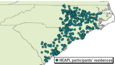
The PM10 (micrograms per cubic meter) and ozone (parts per billion) databases in the study region contained nonuniform data formats and data collection times. A total of 87 PM10 monitoring stations were available during the specified study period (1995–2002). Among them, 75 stations generated observa-tions in terms of 24-hr averages every 6 days, whereas the remaining stations recorded hourly; however, only 15 out of 75 daily and 6 out of 12 hourly monitoring stations were in constant operation during the entire study period. In contrast, all of the 77 ozone moni-toring stations obtained hourly observations, but only 11 stations operated constantly throughout the study period. Figure 1 shows the spatial distribution of the monitoring sta-tions for both pollutants (PM10 and ozone) and the geographic locations of the residences of the study participants.
Residential data source. HEAPL used
extant residential data collected from 620 participants in the Carolina Lupus Study (Cooper et al. 2002). We collected the resi-dential data used in present analyses from the baseline interview that took place in early 1997 to mid-1998 as well as the subsequent interview in 2001. Most participants lived in the eastern and central part of the Carolinas, as shown in Figure 2. To obtain the coor-dinates (longitudes and latitudes), the geo-coding of all study participants’ residential addresses during this period was processed by a specialist at the Cecil G. Sheps Center for Health Services Research at University of North Carolina at Chapel Hill following the standard procedure (Bonner et al. 2003; Ward et al. 2005). The HEAPL study proto-cols have been approved by the Institutional Review Board of the University of North Carolina at Chapel Hill.
BME analysis. The BME theory was
introduced in geostatistics and space–time statistics by Christakos (2000). BME was later considered in a general epistematics con-text and applied in the solution of real-world problems in environmental health fields (Choi et al. 2003; Christakos 2009; Law et al. 2006; Savelieva et al. 2005; Serre et al. 2003). BME analysis can incorporate nonlinear exposure estimators and non-Gaussian probability laws, and it can integrate core knowledge (epide-miologic laws, scientific models, theoretical space–time dependence models, etc.) with multisourced, site-specific information at vari-ous scales (including aggregated variables and empirical relationships). Central elements of the BME method are described below.
A human exposure attribute (e.g., pol-lutant concentration) is represented as a spatiotemporal random field (RF) Xp = Xst Figure 1. Geographic locations of air pollution
mon-itoring stations.
PM10 monitors
Ozone monitors
Figure 2. Geographic locations of HEAPL partici-pants’ residences.
(Christakos and Hristopulos 1998), where the vector p = (s, t) denotes a spatiotemporal point (s is the geographic location and t is the time). The RF model is viewed as the collec-tion of all physically possible realizacollec-tions of the exposure attribute we seek to represent mathematically. It offers a general and math-ematically rigorous framework to investigate human exposure that enhances predictive capability in a composite space–time domain. The RF model is fully characterized by its probability density function (pdf) ƒKB, which
is defined as
PKB[χ1 ≤ Xp1 ≤ χ1 + dχ1,...,χk ≤ Xpk ≤ χk + dχk] = fKB(p1,...,pk)dχ1...dχk, [1] where the subscript KB denotes the “knowl-edge base” used to construct the pdf.
We considered two major knowledge bases: the core (or general) knowledge base, denoted by G-KB, which includes physi-cal and biologiphysi-cal laws, primitive equations, scientific theories, and theoretical models of space–time dependence; and the specifica-tory (or site-specific) knowledge base, S-KB, which includes exact numerical values (hard data) across space–time, intervals (of possi-ble values), and probability functions (e.g., the datum at the specified location has the form of a probability distribution). The total knowledge base is denoted by K = G ∪ S; that is, it includes both the core and the site-specific knowledge bases.
The fundamental BME equation is as follows (for technical details, see Christakos et al. 2005): d χ ∫
(
g − g)
eμTg =0 d χ ξS ∫ eμTg−A fK( )
p =0 ⎫ ⎬ ⎪ ⎭⎪, [2]where g is a vector of gα functions (α = 1, 2, . . . ) that represents stochastically the G-KB under consideration (the bar denotes statistical expectation), µ is a vector of µα-coefficients that depends on the space–time coordinates and is associated with g (i.e., µα expresses the relative significance of each gα function in the composite solution sought), ξS represents the
S-KB available, A is a normalization param-eter, and ƒK is the pollutant or exposure pdf
at each space–time point (the subscript K means that ƒK is based on the total
knowl-edge base that is the blending of the core and site-specific knowledge bases). The vectors g and ξS are inputs in Equation 2, whereas the
unknowns are µ and ƒK across space–time.
The G-KB refers to the entire p domain of interest, which consists of the space–time point vector pk where exposure estimates
are sought and the point vector pdata where site-specific information is available. The G-KB may include theoretical space–time
dependence models (mean, covariance, vario-gram, generalized covariance, multiple-point statistics, and continuity orders) of the expo-sure attribute represented by the RF Xp. Most commonly, however, only the mean and the covariance (or variogram) are used in geosta-tistics studies of human exposure. In addition, the exposure variables of interest are often log-normally distributed. One cannot avoid noticing that there are serious concerns about the biased estimation of the arithmetic mean on the basis of the log-normal assumption (Parkhurst 1998). In our study, we applied the normal score transformation (Deutsch and Journel 1998) to all PM10 and ozone data sets, thus relaxing the log-normal assumption and assuring that the transformed data set is normally distributed.
For practical purposes, the data point vec-tor pdata consists of the hard data point vector phard (where exact measurements are available) and the soft data point vector psoft (where qual-itative/incomplete yet valuable information may be available). For illustration, assume that 32 exact PM10 observations are available at the space–time points phard = (p1,..., p32), that is,
Xp1 = 5.1,..., Xp32 = 9.3 (in suitable units); and that 55 uncertain PM10 data are available at the points psoft = (p33,..., p87), say, of the inter-val form 3.2 < X p33 < 4.1,..., 5.2 < Xp87 < 6.4 (in suitable units). This sort of site-specific information is mathematically expressed by
PS [X p1 = 5.1,..., X p32 = 9.3 ] =1 and PS [3.2
< Xp33 < 4.1,..., 5.2 < Xp87 < 6.4 ] =1, respec-tively. More generally, assume that at point p24 the uncertain datum is expressed by the density function ƒS (p24); then, PS [X p24 < χ ] = ∫χ–∞dχ fS (p24). For several other examples, see Yu et al. (2007).
By incorporating the total K-KB into exposure analysis, the derived pdf ƒK in
Equation 2 describes the distribution of expo-sure values at each estimation point pk. Given
the ƒK at pk, different exposure estimates
(most probable, error minimizing, etc., esti-mates) can be calculated at each spatiotem-poral node of the appropriate mapping grid, depending on the objectives of the study. As mentioned above, in this work the BME method is implemented by means of the pub-licly available SEKS-GUI software library (Kolovos et al. 2006; Yu et al. 2007).
Multiple time-scale exposure. In the
con-text of HEAPL, we considered air pollution exposure at multiple long time scales (includ-ing weekly, monthly, trimonthly, six-monthly, and yearly averages). As described above, the available data sets, which contain either hourly observations or combined daily and hourly observations, are regarded as a realiza-tion of the spatiotemporal RF Xp representing the ambient pollutant, and the space–time dependence of the pollutant is characterized by the joint pdf (1) of the Xp. To estimate
long-term mean exposure, the available short-time-scale data (hourly and daily) should be upscaled to the larger time scale (monthly, yearly, etc.). Spatiotemporal characteristics at short time scales can be also upscaled to rep-resent long-term exposure characteristics that will be incorporated into the BME frame-work, as discussed further below. Spatial and/ or temporal upscaling has been discussed in several environmental health studies (Choi et al. 2003; Christakos and Hristopulos 1998; Gotway and Young 2002).
In the present study, to estimate air pollu-tion exposures at large time scales, we exam-ined two different upscaling methods: daily data aggregation followed by BME estimation at longer time scales (UM1) and daily BME estimation followed by aggregation at longer time scales (UM2).
G-KB. To obtain long-term exposure estimates at the area of interest in terms of the UM1, we first upscaled the data avail-able from the short time scale of observation, (s, t), to the long-time-scale domain, (s, T),
T > t; we then generated estimates of the
upscaled pollutant exposure. Consider the pollutant RF Xp=Xs,t with covariance cX (pi,
pj ) = cX (si, ti; sj, tj) at the (s, t) scale. The
temporally upscaled RF and the correspond-ing covariance at the (s, T) scale are expressed by, respectively,
Xs,T = |T|−1∫T Xs,u du, [3] and
cX(s,T;s´,T ) = (|T|)−2∫T∫TcX (s,u;s´,v)dudv, [4]
where T denotes the time intervals of the upscaled domain within which the original, short-time-scale RF is averaged. Equations 3 and 4 belong to the G-KB of the pollutant. The change of covariance function under a change of support as shown above in spatial analysis is also known as regularization theory (Journel and Huijbregts 1978).
To obtain long-term exposure estimates at the (s, T ) region of interest in terms of the UM2, we first use the BME technique to generate exposure estimates for all locations of interest at the small time scale (s, t), and then obtain the upscaled estimates from the aggre-gation of the short-time-scale estimates. In the UM2 context, the G-KB consists of the mean trend and covariance functions at the short-term time scale (s, t).
S-KB. Daily or hourly observations were aggregated into the multitime scale exposure knowledge base. This upscaled uncertain knowledge base of pollutant concentration is represented in terms of a complete prob-ability distribution rather than a single value. As mentioned above, the sampling frequency generally varies among the monitoring sta-tions. Concerning the raw AQS data set used
in this study, both daily and hourly PM10 observations were available, whereas hourly data were primarily used in the case of ozone. According to the AQS ambient pollutant manual (U.S. EPA 2004), daily observations can be estimated in terms of the arithmetic mean of hourly observations only if the num-ber of these observations is greater than 18 (i.e., ≥ 75% of intended samples); otherwise, we treated them as missing data. Needless to say that, it is not always easy to assure that the long-term exposure information satisfies the 75% criterion above. In fact, the total number of observation days is often less than half the long-term period of interest. Instead of ignoring the scarce observations, as done by the previous methods, in the present study we considered two different avenues toward quantification of the uncertainty of the long-term exposure estimates: (a) for the 25–75% sampling period, data pdfs of various shapes were constructed on the basis of the obser-vation histograms; and (b) for the < 25% sampling period, uniform distributions were generated on the basis of the arithmetic mean. The ranges of the upscaled exposure data were between 0.25 and 1.75 times the arithme-tic mean. If daily and hourly observations coexisted at the same location, the same 24 observed daily values were assigned into the corresponding hours. If daily and hourly observations were collocated, the daily infor-mation was considered to be hard data. In this way, BME was able to account for uncer-tain yet valuable exposure information.
There were 87 (PM10) and 77 (ozone) monitoring stations, but the spatial network of pollution monitors never operated fully during the entire 2,922 days of the study period. In fact, the mean (median) number
of operating stations in any specific day was 15 (8) stations for PM10, and 41 (55) stations for ozone. The maximum (minimum) num-ber of stations per day was 66 (3) for PM10 and 69 (7) for ozone, respectively. Moreover, most of the PM10 stations obtained observa-tions with a 6-day frequency.
Spatiotemporal exposure estimation and
cross-validation. Daily estimation is the
small-est temporal small-estimation unit in this study. The performance of the BME method in daily PM10 and ozone exposure estimation was assessed by cross-validation, using all AQS data available during the study period. Cross-validation allows assessment of the estimation accuracy in different space–time domains and can avoid the potentially biased interpretation of the estimation results induced by purely spatial correlations or purely temporal trends. Therefore, we randomly selected approximately 1,000 observations across space–time to be the estimation points for cross-validation pur-poses. This selection is based on the objective of achieving a balance between three factors: the desirable size of spatiotemporal clusters, the number of clusters (968 for PM10 and 996 for ozone), and the need to reduce the computation burden of the cross-validation of BME estimates at both the daily and the large time scales. The differences of real observations versus BME estimates within each randomly selected spatiotemporal cluster were pooled and assessed across all monitors. For the purpose of comparison, simple kriging with the same spa-tiotemporal structure for BME method, that is, mean trend and covariance, is also applied to the cross-validation at daily scale.
We also applied the cross-validation of large-scale exposure estimation to assess and compare the predictive accuracy by the two
upscaling methods, UM1 and UM2. In UM1, the exposure data were first transformed to the scale of interest, and then the BME technique was applied on the upscaled data, which can be hard or soft, as discussed above, to gener-ate upscaled exposure estimgener-ates. In UM2, on the other hand, the daily exposure G-KB and S-KB were processed, as discussed above, and the daily estimates generated by the BME technique, and then the exposure estimates were upscaled to the domain of interest.
In order to produce the long-term expo-sure estimates, the daily estimates were aggre-gated as follows: Xs,T =T −1 Xs,ti ti∈T
∑
, [5] andσ2X(s,T)=Var T
(
−1∑ti∈TXs,ti)
≈ T−2 σ X 2 s,t i ( )+ σX2(s,T) ⎡⎣ ⎤⎦ ti∈T ∑
{
+2∑ti∈T∑t j ∈TcX(
s,ti;s,tj)}
, [6] where σ2X (s, T) and σ2X (s, ti) are the
vari-ances of Xs,T and Xs,ti, respectively, and cx(s,
ti; s, t j) is the covariance between (s, ti) and
(s, t j). Note that in this study the choice of
the exposure estimation period (T) is differ-ent from that in many epidemiologic studies that followed the calendar temporal units. Instead, we define the exposure period in this study as the period that starts at the time of the epidemiologic survey of the participants and retrospectively defines a specified period of interest, making the exposure time window temporally aligned with the timing of collect-ing health data durcollect-ing the survey.
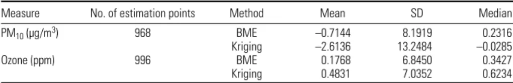
In the case of multiple-time-scale expo-sure, we also conducted two additional cross-validation exercises (one for UM1 and one for UM2) to compare the relative performance of the two upscaling methods at large time scales. The idea of cross-validation is to assess estimation accuracy by comparing the expo-sure estimates with true expoexpo-sure observa-tions. However, the latter are not directly available at long time scales. To overcome this difficulty, statistical hypothesis tests were implemented to detect if the generated soft exposure data are significantly close to the BME exposure estimates. The “distance” between the pdfs of soft data and the BME Table 1. BME and kriging cross-validation results (statistics of estimation errors for daily estimates).
Measure No. of estimation points Method Mean SD Median
PM10 (µg/m3) 968 BME –0.7144 8.1919 0.2316
Kriging –2.6136 13.2484 –0.0285
Ozone (ppm) 996 BME 0.1768 6.8450 0.3427
Kriging 0.4831 7.0352 0.6234
Table 2. Summary statistics of the cross-validation results for the BME long-term exposure estimates derived by UM1 and UM2.
UM1 UM2
Time period Mean Median SD Mean Median SD
PM10 1 Week –2.8944 –3.2590 7.8800 –1.9057 –1.1636 7.9308 1 Month –3.1889 –2.0855 7.2113 –2.4693 –1.2410 7.1029 3 Months –3.2260 –2.1502 6.9366 –2.5038 –1.0816 7.0235 6 Months –3.2732 –2.2481 7.0015 –2.2868 –0.7581 6.8586 1 Year –3.0810 –3.2590 6.5565 –2.2919 –1.3173 6.4123 Ozone 1 Week 1.9795 1.9350 4.9122 2.3559 2.4536 5.1754 1 Month 1.6399 1.6287 4.2774 1.5039 1.8269 4.2932 3 Months 2.1265 2.4236 4.1578 0.7233 1.1856 4.3105 6 Months 2.4861 2.8128 4.0799 –0.5237 –0.2164 4.3031 1 Year 2.4537 2.9891 3.7602 –1.3781 –0.7395 3.8705
Table 3. Percentage of successful cross-validation results of long-term exposure estimation.
Time PM10 Ozone
period UM1 (%) UM2 (%) UM1 (%) UM2 (%)
1 Week 10.16 11.18 74.60 55.89
1 Month 71.49 74.54 54.15 61.71
3 Months 76.11 77.38 64.87 95.78
6 Months 77.66 79.18 81.64 95.41
estimates was assessed in terms of the relative entropy measure:
I p,q
(
)
=∑
k=1n pklog p(
k qk)
, [7] where pk and qk represent the pdfs of theexposure observations and the BME estimates, respectively. The goodness-of-fit test is usually applied to verify if the two pdfs come from the same random variable. Chi-square dis-tribution with n – 1 degrees of freedom can be used in the relative entropy measure tests (Bedford and Cooke 2001). The significance criterion for the tests was set as 95%. Cross-validation for the UM1 and UM2 methods at long time scales was performed at the same temporally-referenced points as in the case for the cross-validation of daily BME estimation.
Finally, we applied both UM1 and UM2 to estimate PM10 and ozone exposures at multiple time scales for all the residential loca-tions of the HEAPL study. The correlation
coefficients for each BME estimate at differ-ent time scales were computed for the UM1 and UM2 methods and compared accord-ingly. We also examined the distribution of the differences between the UM1 and UM2 estimates at different time scales.
Numerical Results and Plots
Table 1 presents the cross-validation results for the daily PM10 and ozone data by BME and kriging methods. The exposure estima-tion error at each test point is defined as error = estimate – observation. In general, both the error mean and median are close to zero, so the error distribution is symmetric around zero. To compare the average exposures at multiple time scales from real observations versus the BME estimates, Tables 2 and 3 show the results from UM1 and UM2. Table 2 summarizes simple statistics of the esti-mation errors given by UM1 and UM2 for both PM10 and ozone, and Table 3, results ofcorresponding comparison on relative entropy at each indicated time scale, showing the percentage of the spatiotemporal estimates that passed the chi-square tests with the null hypothesis: the two pdfs (data and estimates) are the same.
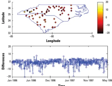
Figures 3–6 show the spatial and temporal distributions of the average estimation errors of the yearly exposure estimates obtained by UM1 and UM2. Figures 3 and 4 show the PM10 estimation performance by means of UM1 and UM2, respectively. Similarly, Figures 5 and 6 show the average error dis-tributions of ozone estimation obtained by UM1 and UM2, respectively.
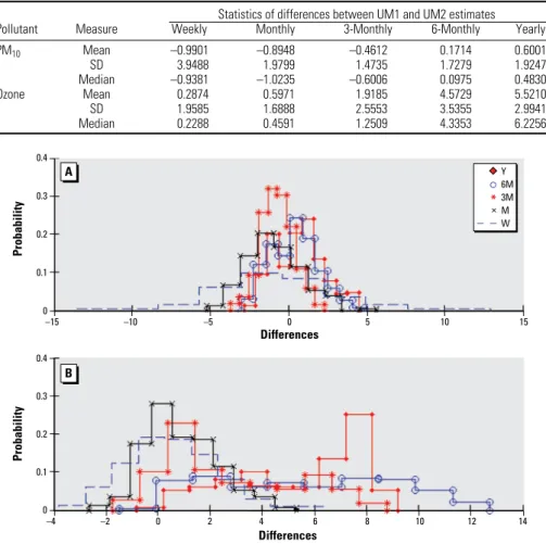
Table 4 presents the summary statistics for the calculated differences in UM1–UM2 that were tabulated, respectively, for PM10 and ozone exposure at each indicated time scale. Figure 7 shows the histograms of these differences for both methods. Table 5 shows the correlation coefficients between the PM10
Figure 3. Spatiotemporal yearly PM10 estimation errors (estimated – observed)
by UM1. 37 36 35 34 33 32 Latitude –85 –80 –75 20 10 0 –10 –20 20 10 0 –10 –20 Differences
Jan 1996 May 1997 Oct 1998 Mar 2000 Jul 2001 Dec 2002 Time
Longitude
Figure 5. Spatiotemporal yearly ozone estimation errors (estimated – observed) by UM1. 37 36 35 34 33 32 Latitude –85 –80 –75 20 10 0 –10 –20 20 10 0 –10 –20 Differences Longitude
Jan 1996 Jun 1996 May 1998
Time
Dec 1996 Jun 1997 Nov 1997
Figure 4. Spatiotemporal yearly PM10 estimation errors (estimated – observed)
by UM2. 37 36 35 34 33 32 Latitude –85 –80 –75 20 10 0 –10 –20 20 10 0 –10 –20 Differences Longitude
Jan 1996 May 1997 Oct 1998 Mar 2000 Jul 2001 Dec 2002 Time
Figure 6. Spatiotemporal yearly ozone estimation errors (estimated – observed) by UM2. 37 36 35 34 33 32 Latitude –85 –80 –75 20 10 0 –10 –20 20 10 0 –10 –20 Differences Longitude
Jan 1996 Jun 1996 May 1998
Time
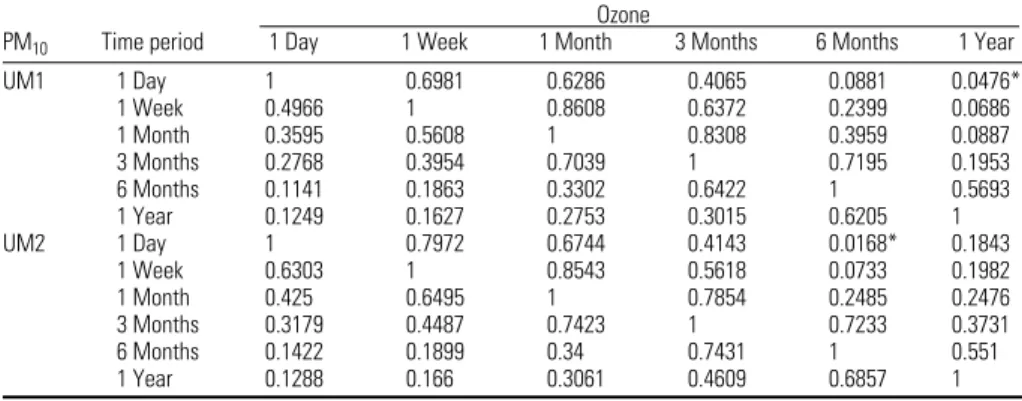
and ozone exposure estimates obtained by UM1 and UM2 within each temporal scale at the study residences.
Discussion
Scale laws and scaling behaviors at multiple time scales are encountered in many human exposure scenarios, although very often such laws are found in an empirical way, because of the lack of fundamental theories allowing us to understand them from fundamental principles (Christakos and Hristopulos 1998). In the case of chronic diseases, the arithmetic mean of long-term (large time scale) partici-pant exposure rather than the on-site exposure is often considered as the appropriate indicator (AckermannLiebrich et al. 1997; Pope et al. 2002). For regulatory purposes, the National Ambient Air Quality Standards (NAAQS) pro-posed by U.S. EPA are also based on the arith-metic mean exposure at different time scales, which range from hourly to annual exposure (U.S. EPA 2006). Many studies have focused on long-term arithmetic mean exposure esti-mates based on small time scale (short-term) observations and assuming lognormal RF to model exposure distributions (Clayton et al.
1999; Wallace and Williams 2005). In general, these studies do not consider important spa-tiotemporal dependencies between short-term observations and cross-dependencies between short- and long-term exposures.
In this article, we present two upscaling methods and compare them for the estima-tion of arithmetic average exposures within the different temporal scales. As described in the introductory remarks, previous data anal-yses often did not consider the uncertainty of the exposure analysis (e.g., by purely spatial or purely temporal analysis or linear assump-tions). For the upscaling problem considered here, this uncertainty may be a significant factor in many human exposure situations; for example, in the case of PM10 data with a distinct trend and a large number of missing values (because most monitors only record every 6 days), the estimation of the long-term exposure averages can be seriously biased.
As mentioned above, the AQS manual suggests that when there is a large number of missing data the accuracy of the upscaled exposure is in doubt, in which case the rest of the observed information should be ignored. Accordingly, mainstream statistics
and geostatistics techniques usually consider incomplete information (qualitative knowl-edge, uncertain secondary records, etc.) as missing data to avoid potentially misleading estimation results. On the other hand, the BME method used in this study has the signif-icant feature that it is able to rigorously incor-porate uncertain information of various kinds and different scales with the minimum num-ber of theoretical assumptions. In other words, the BME method can always express incom-plete information in terms of soft site-specific data that can take the form, for example, of probability functions with arbitrary shapes. In addition, BME can incorporate empirical rela-tions and charts as well as core knowledge in the form of epidemiologic laws and scientific human exposure models, whenever available (Christakos et al. 2005). Because of the abun-dance of missing data, the uncertain (soft) information is available for both PM10 and ozone BME predictions at all concerned time scales in this study. Table 1 provides the cross-validation results of daily PM10 and ozone estimations by BME and kriging methods and shows that the estimation error distribution of the results of BME method is more condensed and symmetric around zero. The improvement of the estimation accuracy by integrating soft data in BME method is more significant as the amount of missing data is greater, such as the case of PM10.
Concerning the comparison of the accura-cies of the two upscaling approaches: based on the cross-validation results (Table 2 and 3), the UM2 is generally better than UM1 in terms of smaller mean and median errors and higher success rates of passing the chi-square tests of uncertain information. Table 2 shows that the standard deviation of the differences between observations and estimates decreases as the estimation time scale increases (for both PM10 and ozone cases). This is because the aggregated hard and soft data (which emerge as the time scale increases) can lead to a reduc-tion of the estimareduc-tion uncertainty and provide more informative exposure estimates. In the case of the PM10 data set, for example, dur-ing the study period of interest about 5,000 more spatiotemporal data are compiled in the yearly database than in the weekly data-base. The UM1 and UM2 methods gener-ally underestimate the real PM10 levels. The preferential sampling of high PM10 values can partially contribute to the biased estimations. Also, some extreme high values in PM10 data set can also bias the estimations at the process of normal score transform.
Geostatistical techniques generate estimates in terms of spatial and temporal interpolation schemes, which rely on linearity and normal-ity assumptions and tend to generate rather smooth PM10 estimates. On the other hand, the UM1 and UM2 use the BME approach Figure 7. Abbreviations: M, 1 month; 3M, 3 months; 6M, 6 months; W, 1 week; Y, 1 year.
Distribution of differences between the UM1 and UM2 exposure estimates for PM10 (A) and ozone (B) at
multiple time scales.
0.4 0.3 0.2 0.1 0 Probability –15 –10 –5 0 5 10 15 Differences Y 6M 3M M W * × 0.4 0.3 0.2 0.1 0 Probability Differences –4 –2 0 2 4 6 8 10 12 14 A B
Table 4. Summary statistics of the differences between UM1 and UM2 estimates of PM10 and ozone given
for all residential locations.
Statistics of differences between UM1 and UM2 estimates
Pollutant Measure Weekly Monthly 3-Monthly 6-Monthly Yearly
PM10 Mean –0.9901 –0.8948 –0.4612 0.1714 0.6001 SD 3.9488 1.9799 1.4735 1.7279 1.9247 Median –0.9381 –1.0235 –0.6006 0.0975 0.4830 Ozone Mean 0.2874 0.5971 1.9185 4.5729 5.5210 SD 1.9585 1.6888 2.5553 3.5355 2.9941 Median 0.2288 0.4591 1.2509 4.3353 6.2256
that does not make any linearity or normality assumption (nonlinear estimators and non-Gaussian distributions are automatically incor-porated) and can rigorously process uncertain yet valuable data sources (e.g., soft data of vari-ous forms), thus providing more informative estimates than the geostatistical techniques.
In the case of highly uncertain data, some extremely high observations may not be com-pletely reproduced. Even though both upscal-ing methods underestimate the actual PM10 exposures, the UM2 performs better than UM1 yielding lower estimation errors. In the case of ozone, the performance of UM1 is sig-nificantly different than that of UM2. UM1 tends to overestimate the long-term exposure level, and the situation worsens as the esti-mation scale becomes larger. Remarkably, the UM2 exposure estimates are not biased, whereas the biased UM1 estimation is likely due to the aggregation of the ozone data set. Because of the seasonal ozone pattern, the dis-tribution of daily ozone data during the study period is positively skewed, ranging from 0 to 70 ppb. However, when temporal aggregation was applied, the mean of the upscaling data generally raised to the annual mean level at each spatial location, which may distort the original spatiotemporal ozone pattern at the smaller time scales. As shown in Figure 8, the distribution of the mean of the aggregated ozone data varies significantly by the degree of upscaling, which is not the case of the PM10 estimation. Moreover, UM2 does not depend on any distorted upscaled data, so more accurate results are obtained. Despite the significant changes in data structure during aggregation, the rigorous consideration of data uncertainty by BME alleviates such effects to produce better quality estimates (Table 2). Table 3 shows that the estimates are gener-ally superior for ozone than for PM10. This is because most PM10 monitors performed air sampling every 6 days, in which case the resulting upscaled long-term exposure is less informative of the exposure situation, espe-cially at the short time scales. Therefore, the shorter the upscaling period considered (e.g., weekly), the more noninformative uncertain data are compared with estimations.
Figures 3–6 plot the spatial and temporal distributions of the UM1 and UM2 results. In the PM10 case, the spatial and temporal patterns of the error distributions obtained by the UM1 and UM2 methods are very similar. These plots offer a better understanding of the performance of the proposed approach in space–time. The conclusion drawn from Table 2 concerning long-term PM10 underestima-tion is also illustrated by the temporal error distributions plotted in figures 3–6. In the case of ozone estimation, these figures also depict a similar conclusion drawn from Table 2 (i.e., UM1 tends to overestimate the long-term
ozone levels). It is noteworthy that spatial locations where the estimates exhibit higher discrepancies from the data values (for both PM10 and ozone) are mostly close to either the boundary between regions of considerable data availability and data scarcity or the metro-politan area where the high variability of PM pollutants and ozone generated from traffic or local industrial emissions may be present.
The mean and median of the differences between the UM1 and UM2 estimates spe-cific to the residential locations in HEAPL at multiple timescales are mostly close to each other and not much departing from zero for both pollutants (Table 4), except in the case of long-term ozone estimation. The estimates obtained by UM1 are biased, so UM1 gener-ates higher ozone levels than UM2, which can be seen more clearly from the histograms at the bottom of Figure 7. In general, the UM1 and UM2 estimates should get closer to each other as the time scale increases under
the condition of the unbiased aggregated data provided. As the time scale increases, the number of daily values increases for both upscaling methods (i.e., more data become available for aggregation purposes in the case of UM1, whereas more estimates are gener-ated for integration purposes in the case of UM2). As a consequence, based on the central limit theorem, the exposure mean is optimally calculated at the longer time scale by both upscaling methods (Figure 8), as shown in the case of PM10 estimation. However, the expo-sure estimation accuracy may also decrease if the data uncertainty resulting from the large proportion of missing data or biased aggre-gated data is large, which is the case of ozone estimation at long time scales. Thus, the mean and median of the differences between the estimation results by UM1 and UM2 can slightly increase with time scale.
In this study, numerical analysis showed that UM2 generally performs slightly better Table 5. Correlation coefficients among multitemporal-scale exposure estimations for PM10 and ozone.
Ozone
PM10 Time period 1 Day 1 Week 1 Month 3 Months 6 Months 1 Year
UM1 1 Day 1 0.6981 0.6286 0.4065 0.0881 0.0476* 1 Week 0.4966 1 0.8608 0.6372 0.2399 0.0686 1 Month 0.3595 0.5608 1 0.8308 0.3959 0.0887 3 Months 0.2768 0.3954 0.7039 1 0.7195 0.1953 6 Months 0.1141 0.1863 0.3302 0.6422 1 0.5693 1 Year 0.1249 0.1627 0.2753 0.3015 0.6205 1 UM2 1 Day 1 0.7972 0.6744 0.4143 0.0168* 0.1843 1 Week 0.6303 1 0.8543 0.5618 0.0733 0.1982 1 Month 0.425 0.6495 1 0.7854 0.2485 0.2476 3 Months 0.3179 0.4487 0.7423 1 0.7233 0.3731 6 Months 0.1422 0.1899 0.34 0.7431 1 0.551 1 Year 0.1288 0.166 0.3061 0.4609 0.6857 1 *p > 0.05.
Figure 8. Distribution of means of upscaled PM10 (A) and ozone (B) data.
0.08 0.06 0.04 0.02 0 Probability 0 20 Concentration (µg/m3) 40 60 80 100 120 140 160 180 0.20 0.15 0.10 0.05 0 Probability Concentration (ppm) 0 10 20 30 40 50 60 70 80 90 100 Daily 3-monthly Yearly × + A B
than UM1 in terms of accuracy. UM2 can also be preferable in theory. Instead of aggregating the data and spatiotemporal dependence at small scales, BME analysis incorporates G-KB and S-KB, including detailed local spatiotem-poral associations and the original short-term observations. In UM1, on the other hand, both general and specific knowledge are upscaled, so the BME estimation uses the more uncertain information. However, despite the better performance of UM2, in practice the UM1 may be sometimes preferable because of its efficiency. The difference of compu-tation burden between the two approaches increases substantially as the estimation time scale increases. As the exposure estimation at residential locations shows, the UM1 can gen-erate biased estimates in the case of ozone but not in the case of PM10. This suggests the cri-terion for the selection of UM1 and UM2 in the long-term exposure estimations. UM1 is preferable as long as the aggregation process does not change the original data structure, that is, mean trend and variance/covariance of the data. In such cases, the loss of informa-tion during the data aggregainforma-tion in UM1 can be neglected compared with the increase of time for the estimations by UM2; otherwise, UM2 is preferable. In this study, because of the strong seasonal ozone trend, an aggrega-tion period exceeding 3 months can distort the spatiotemporal data structure.
Conclusions
To estimate residential levels of exposure to ambient air pollution in a community-based study, in this article we presented and com-pared two BME-based temporal upscaling methods (UM1: data aggregation followed by BME estimation; and UM2: BME estimation followed by aggregation). BME’s flexibility allowed the assimilation of G-KB and S-KB of different formats; for example, BME expo-sure analysis can process scarce and uncer-tain data sets in a probabilistic way, instead of neglecting them, as is the case with most existing quantitative exposure methods. In the context of residential long-term exposure estimation, we showed that the UM1 and UM2 methods produce accurate space–time estimates. By means of cross-validation tests the relative performance of the two upscaling methods was studied in different time scales. We found UM2 to be generally better than UM1, in the sense that the UM2 estimates were unbiased, the differences between the UM2 estimates and the true long-term expo-sures were smaller, and the UM2 exhibited better test-passing rates than UM1. On the other hand, the UM1 can perform reason-ably well when the aggregation process does not alter the spatiotemporal structure of the original data set.
RefeRences
AckermannLiebrich U, Leuenberger P, Schwartz J, Schindler C, Monn C, Bolognini C, et al. 1997. Lung function and long term exposure to air pollutants in Switzerland. Am J Respir Crit Care Med 155(1):122–129.
Aickin M. 2002. Causal Analysis in Biomedicine and Epidemiology: Based on Minimal Sufficient Causation. New York:Marcel Dekker.
Bedford T, Cooke RM. 2001. Probabilistic Risk Analysis: Foundations and Methods. Cambridge, UK:Cambridge University Press. Bonner MR, Han D, Nie J, Rogerson P, Vena JE, Freudenheim AL.
2003. Positional accuracy of geocoded addresses in epide-miologic research. Epidemiology 14(4):408–412.
Brauer M, Hoek G, van Vliet P, Meliefste K, Fischer P, Gehring U, et al. 2003. Estimating long-term average particulate air pollution concentrations: application of traffic indicators and geographic information systems. Epidemiology 14(2):228–239. Chen CC, Wu KY, Chang MJW. 2004. A statistical assessment
on the stochastic relationship between biomarker concen-trations and environmental exposures. Stoch Environ Res Risk Assess 18(6):377–385.
Choi KM, Serre ML, Christakos G. 2003. Efficient mapping of California mortality fields at different spatial scales. J Expo Anal Environ Epidemiol 13(2):120–133.
Christakos G. 2000. Modern Spatiotemporal Geostatistics. New York:Oxford University Press.
Christakos G. 2009. Epistematics: An Evolutionary Framework of Real World Problem-Solving. New York:Springer. Christakos G, Hristopulos DT. 1998. Spatiotemporal Environmental
Health Modelling: A Tractatus Stochasticus. Boston:Kluwer Academic.
Christakos G, Olea RA, Serre ML, Yu H-L, Wang L. 2005. Interdisciplinary Public Health Reasoning and Epidemic Modelling: The Case of Black Death. New York:Springer. Christakos G, Serre ML. 2000. BME analysis of spatiotemporal
particulate matter distributions in North Carolina. Atmos Environ 34(20):3393–3406.
Christakos G, Serre ML, Kovitz JL. 2001. BME representation of particulate matter distributions in the State of California on the basis of uncertain measurements. Geophys Atmos 106(D9):9717–9731.
Christakos G, Thesing GA. 1993. The intrinsic random-field model in the study of sulfate deposition processes. Atmos Environ A Gen 27(10):1521–1540.
Christakos G, Vyas VM. 1998. A composite space/time approach to studying ozone distribution over Eastern United States. Atmos Environ 32(16):2845–2857.
Clayton CA, Pellizzari ED, Rodes CE, Mason RE, Piper LL. 1999. Estimating distributions of long-term particulate mat-ter and manganese exposures for residents of Toronto, Canada. Atmos Environ 33(16):2515–2526.
Conceicao GMS, Miraglia SGEK, Kishi HS, Saldiva PHN, Singer JM. 2001. Air pollution and child mortality: a time-series study in Sao Paulo, Brazil. Environ Health Perspect 109:347–350. Cooper GS, Dooley MA, Treadwell EL, St Clair EW, Gilkeson GS.
2002. Hormonal and reproductive risk factors for development of systemic lupus erythematosus: results of a population-based, case-control study. Arthritis Rheum 46(7):1830–1839. Deutsch CV, Journel AG. 1998. GSLIB Geostatistical Software
Library and User’s Guide [CD]. New York:Oxford University Press.
Gotway CA, Young LJ. 2002. Combining incompatible spatial data. Am Stat Assoc 97(458):632–648.
Hoek G, Fischer P, Van den Brandt P, Goldbohm S, Brunekreef B. 2001. Estimation of long-term average exposure to outdoor air pollution for a cohort study on mortality. J Expo Anal Environ Epidemiol 11(6):459–469.
Journel AG, Huijbregts CJ. 1978. Mining Geostatistics. New York:Academic Press.
Katsouyanni K, Pershagen G. 1997. Ambient air pollution expo-sure and cancer. Cancer Causes Control 8(3):284–291. Kentel E, Aral MM. 2005. 2D Monte Carlo versus 2D fuzzy
Monte Carlo Health Risk Assessment. Stoch Environ Res Risk Asses 19(1):86–96.
Kolovos A, Yu H-L, Christakos G. 2006. SEKS-GUI v.0.6. User’s Manual-06 Ed. San Diego, CA:Department of Geography, San Diego State University.
Law DCG, Bernstein KT, Serre ML, Schumacher CM, Leone PA, Zenilman JM, et al. 2006. Modeling a syphilis outbreak through space and time using the Bayesian maximum entropy approach. Ann Epidemiol 16(11):797–804. Li HL, Huang GH, Zou Y. 2008. An integrated fuzzy-stochastic
modeling approach for assessing health-impact risk from air pollution. Stoch Environ Res Risk Assess 22(6):789–803. Liao DP, Peuquet DJ, Duan YK, Whitsel EA, Dou JW, Smith RL,
et al. 2006. GIS approaches for the estimation of residential-level ambient PM concentrations. Environ Health Perspect 114:1374–1380.
Maxwell RM, Kastenberg WE. 1999. A model for assessing and managing the risks of environmental lead emissions. Stoch Environ Res Risk Assess 13(4):231–250.
Michelozzi P, Capon A, Kirchmayer U, Forastiere F, Biggeri A, Barca A, et al. 2002. Adult and childhood leukemia near a high-power radio station in Rome, Italy. Am J Epidemiol 155(12):1096–1103.
Mutshinda CM, Antai I, O’Hara RB. 2008. A probabilistic approach to exposure risk assessment. Stoch Environ Res Risk Assess 22(4):441–449.
Nyberg F, Gustavsson P, Jarup L, Bellander T, Berglind N, Jakobsson R, et al. 2000. Urban air pollution and lung can-cer in Stockholm. Epidemiology 11(5):487–495.
Ozkaynak H, Xue J, Spengler J, Wallace L, Pellizzari E, Jenkins P. 1996. Personal exposure to airborne particles and metals: results from the particle team study in Riverside, California. J Expo Anal Environ Epidemiol 6(1):57–78.
Parkhurst DF. 1998. Arithmetic versus geometric: means for environmental concentration data. Environ Sci Technol 32(3):92a–98a.
Pope CA, Burnett RT, Thun MJ, Calle EE, Krewski D, Ito K, et al. 2002. Lung cancer, cardiopulmonary mortality, and long-term exposure to fine particulate air pollution. JAMA 287(9):1132–1141.
Rushton G, Krishnamurthy R, Krishnamurti D, Lolonis P, Song H. 1996. The spatial relationship between infant mortality and birth defect rates in a US city. Stat Med 15(17–18):1907–1919. Sagiv SK, Mendola P, Loomis D, Herring AH, Neas LM, Savitz DA,
et al. 2005. A time-series analysis of air pollution and preterm birth in Pennsylvania, 1997–2001. Environ Health Perspect 113:602–606.
Savelieva E, Demyanov V, Kanevski M, Serre M, Christakos G. 2005. BME-based uncertainty assessment of the Chernobyl fallout. Geoderma 128(3–4):312–324.
SEKS-GUI. 2007. Spatiotemporal Epistematics Knowledge Synthesis Model - Graphic User Interface. Available: http:// homepage.ntu.edu.tw/~hlyu/software/SEKSGUI/SEKSHome. html [accessed 10 March 2009].
Serre ML, Kolovos A, Christakos G, Modis K. 2003. An applica-tion of the holistochastic human exposure methodology to naturally occurring arsenic in Bangladesh drinking water. Risk Anal 23(3):515–528.
Stallard N, Whitehead A. 1995. The fixed-dose procedure and the acute-toxic-class method: a mathematical comparison. Hum Exp Toxicol 14(12):974–990.
Tamborini P, Sigg H, Zbinden G. 1990. Acute toxicity testing in the nonlethal dose range—a new approach. Regul Toxicol Pharmacol 12(1):69–87.
U.S. EPA (Environmental Protection Agency). 2002. Technology Transfer Network: Air Quality System (AQS). Available: http:// www.epa.gov/ttn/airs/airsaqs/ [accessed 1 March 2007]. U.S. EPA. 2004. AQS Raw Data Summary Formulas Draft.
Washington, DC:U.S. Environmental Protection Agency. U.S. EPA. 2005. AQS Data Coding Manual v2.12. Washington,
DC:U.S. Environmental Protection Agency.
U.S. EPA. 2006. National Ambient Air Quality Standards (NAAQS). Washington, DC:U.S. Environmental Protection Agency. Vyas VM, Christakos G. 1997. Spatiotemporal analysis and
map-ping of sulfate deposition data over eastern USA. Atmos Environ 31(21):3623–3633.
Wallace L, Williams R. 2005. Validation of a method for estimat-ing long-term exposures based on short-term measure-ments. Risk Anal 25(3):687–694.
Wang JF, Christakos G, Han WG, Meng B. 2008. Data-driven exploration of “spatial pattern-time process-driving forces” associations of SARS epidemic in Beijing, China. J Public Health (Oxf) 30(3):234–244.
Ward MH, Nuckols JR, Giglierano J, Bonner MR, Wolter C, Airola M, et al. 2005. Positional accuracy of two methods of geocoding. Epidemiology 16(4):542–547.
Wu J, Wang J, Meng B, Chen G, Pang L, Song X, et al. 2004. Exploratory spatial data analysis for the identification of risk factors to birth defects. BMC Public Health 4:23; doi:10.1186/1471-2458-4-23 [Online 18 June 2004]. Yu HL, Kolovos A, Christakos G, Chen JC, Warmerdam S, Dev B.
2007. Interactive spatiotemporal modelling of health systems: the SEKS-GUI framework. Stoch Environ Res Risk Assess 21(5):555–572.