複雜環境之影像式碰撞濾除運算

(1)

國

立

交

通

大

學

資訊科學與工程研究所

碩

士

論

文

複雜環境之影像式碰撞濾除運算

A Practical Collision Filtering for Complex Environments

Using Image-based Techniques

研究生：陳勇誠

指導教授：莊榮宏教授

(2)

複雜環境之影像式碰撞濾除運算

A Practical Collision Filtering for Complex Environments Using

Image-based Techniques

研究生：陳勇誠 Student：Yong-Cheng Chen

指導教授：莊榮宏 Advisor：Jung-Hong Chuang

國立交通大學

資訊科學與工程研究所

碩士論文

A Thesis

Submitted to Institute of Computer Science and Engineering College of Computer Science

National Chiao Tung University in partial Fulfillment of the Requirements

for the Degree of Master

in

Computer Science

June 2006

Hsinchu, Taiwan, Republic of China

(3)

複雜環境之影像式碰撞濾除運算

學生：陳勇誠指導教授: 莊榮宏博士

國立交通大學資訊工程學系

摘要

我們設計一個可快速且有效率的對複雜場景進行碰撞偵測的演算法，我們將針對影像式的碰撞濾除加以改進並將潛在碰撞集合(potentially colliding set, PCS)分割成數個子集合。在方法中我們延續 CULLIDE 的演算法[13]，在線性時間將那些屬於完全可見的物體從潛在碰撞集合內移除，並且我們在兩次的繪圖流程都給定一個從遠到近的順序，這將大幅度的降低因物體投影重疊而影響方法的效率；儘管有些無發生碰撞的物體被其他的物體給遮蓋著，在我們方法中大多情況下仍能有效濾除。另外，在執行能見度分析也同時計算是否存在分割曲面於潛在碰撞集合中，分割曲面可將潛在碰撞集合分割成數個小的集合，可減少配對碰撞偵測的次數。最後，我們利用 50~200 個由 800 個三角形構成的圓環測試執行效能，平均所花費的碰撞偵測時間約為 0.85~7 秒，實驗結果，證實我們的方法能有效率地應用於物理模擬或即時系統之中

(4)

A Practical Collision Filtering for Complex Environments

using Image-based Techniques

Student: Yong-Cheng Chen

Advisor: Dr. Jung-Hong Chuang

Department of Computer Science and Information Engineering

National Chiao Tung University

ABSTRACT

We present an algorithm for efficient and exact collision detection between complex geo-metric models in large environments using graphics hardware. The purpose of our algo-rithm is to improve image-based collision culling and partition the potentially colliding set (PCS) into subsets. Our algorithm eliminates objects which are fully visible in PCS using occlusion query in linear time. It is based on CULLIDE and decides an order of rendering to supply a more efficient culling performance. We can conspicuously reduce the extent of culling to rely on the depth complexity of the scene along the view direction. Despite there are some collision-free objects are occluded by other objects, they may be pruned in our al-gorithm. Furthermore, our algorithm determines whether separating surfaces exist between the subsets of the PCS. The computation of collision pairs would be beneficial to divide the PCS into multiple sets during the collision culling. Finally, we measured the performance of our algorithm using 50-200 torii with 800 triangles. The average collision detection time is around 0.85-7 milliseconds. In the experiments, our approach had shown to be efficient for collision detection in physics simulation and applied to real-time applications.

(5)

3.4.1 Bounding Volume Hierarchy Construction . . . 29 3.4.1.1 Bounding Volume Hierarchy Optimization . . . 36 3.4.2 Sorting and collision independent sets construction . . . 37 4 Results 39 4.1 Performance analysis in simple environment . . . 40 4.2 Performance comparison for environments of high geometry complexity

and low depth complexity . . . 45 4.3 Performance comparison for environments of high depth complexity and

low geometry complexity . . . 48 5 Conclusion 57 5.1 Summary . . . 57 5.2 Future work . . . 58 Bibliography 59

(7)

List of Figures

2.1 Passible Z-interval cases[BWS99] . . . 7

2.2 Passible Z-interval cases[BWS99] . . . 9

2.3 Semi-infinite rays from a point in a closed mesh[KP03] . . . 9

2.4 Update the depth buffer[KP03] . . . 10

2.5 Increases the stencil buffer when rendering ”front-facing” polygons[KP03]. 10 2.6 Decreases the stencil buffer when rendering ”back-facing” polygons[KP03]. 11 2.7 (a) VoI for A and B; (b) Extended VoI to obtain an outside face for A[HTG03]. 12 2.8 LDI for two pixels, unsorted and sorted with respect to depth values[HTG03]. 13 2.9 Intersection volume for Knot and Dragon[HTG03] . . . 14

3.1 The flowchart of the proposed collision detection system. . . 17

3.2 The worst case of CULLIDE: (a) It shows that there are no intersections in the environment; (b) All the projections of objects overlap with each other; (C) We only can prune the object C using visibility-based pruning in CULLIDE. . . 19

3.3 Projection and sorting. . . 20

3.4 The result of our collision culling: (a) It shows that there are no intersec-tions in the environment; (b) All the projecintersec-tions of objects overlap with each other; (c),(d) There are no occlusion in two passes. . . 22

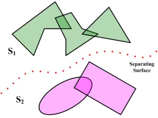
3.5 If S1and S2do not collide with each other, we can find a separating surface among them. . . 23

3.6 (a) Collision independent set; (b) The projection of green objects overlap with the collision independent set, and the projection of yellow objects dose not overlap with the set. . . 24

(8)

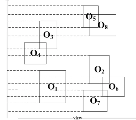
3.7 An example for collision independent sets construction. . . 26 3.8 An example, a scene consists of O1, O2, O3, O4, O5, O6, O7, and O8. . . 30

3.9 Traverse projection elements of e5, e9, and e3. The global probing surface

P Sg is updated to b3. . . 30

3.10 Traverse projection elements of b5 and b8, collision independent set CIS1

is constructed at O8. . . 31

3.11 Traverse projection elements of e4 and b3, and the expansion of CIS1 is

finish at b3. . . 31

3.12 Traverse projection elements of e2 and b4, collision independent set CIS2

3.13 Traverse projection elements of e1, e6 and b2, and the expansion of CIS2

is finish at b2. . . 32

3.14 Traverse projection elements of e7 and b6, collision independent set CIS3

3.15 After the first pass, three independent colliding sets, P CS1 = {O8}, P CS2 =

{O4}, and P CS3 = {O6, O7}, and three separating surfaces, SS1, SS2,

SS3, are found. . . 33

3.16 After the second pass, the three collision independent sets will be finalized as CIS1 = {O5, O8}, CIS2 = {O3, O4}, and CIS3 = {O2, O6, O7}, and

there are two separating surfaces found. . . 34 3.17 Bounding volume hierarchy with a 8-ary tree. . . 36 3.18 Bounding volume hierarchy construction using (a) three eigenvectors of the

covariance matrix; (b) optimizing principal components . . . 37 4.1 Figures (a)-(f) show the simulating process in environment 1. . . 41 4.2 Performance comparison between our approach and CULLIDE in

environ-ment 1. . . 42 4.3 Performance comparison with CULLIDE, CULLIDE with hierarcical

bound-ing volume, and our approach in environment 1 at frame buffer resolution 800×800. . . 43 4.4 The number of collision independent sets constructed for environment 1 at

frame buffer resolution 800×800. . . 44 4.5 Figures (a)-(f) show the simulating process in environment 2. . . 46

(9)

4.6 Performance comparison between our approach and CULLIDE in environ-ment 2. . . 47 4.7 Performance comparison with CULLIDE, CULLIDE with hierarcical

bound-ing volume, and our approach in environment 2 at frame buffer resolution 800×800. . . 49 4.8 Performance comparison between CULLIDE with hierarcical bounding

volume and our approach in environment 2 at frame buffer resolution 800×800. 50 4.9 The number of collision independent constructed for in environment 2 at

frame buffer resolution 800×800. . . 51 4.10 Figure shows the simulating process in environment 3. . . 52 4.11 Performance comparison between our approach and CULLIDE in

environ-ment 3. . . 53 4.12 Performance comparison with CULLIDE, CULLIDE with hierarcical

bound-ing volume, and our approach in environment 3 for 200 torii at frame buffer resolution 800×800. . . 55 4.13 The number of collision independent sets constructed for environment 3

for 200 torii at frame buffer resolution 800×800. . . 56

(10)

List of Algorithms

2.1 The logical flow of RECODE . . . 8

2.2 The algorithm of collision culling . . . 15

3.1 Our collision culling algorithm . . . 21

3.2 The algorithm of collision independent sets construction . . . 35

(11)

List of Tables

3.1 Parameters of collision independent sets construction . . . 27

4.1 Timing statistics for environment 1. . . 45

(12)

Acknowledgments

I would like to thank my advisors, Professor Jung-Hong Chuang, for his guidance, in-spirations, and encouragement. I am grateful to Tan-Chi Ho for his comments and advices. Thanks to my colleagues in CGGM lab.: Yi-Chun Lin, Chao-Wei Juan, Roger Hong, Chen-Li Hao, Yu-Shuo Chen-Lio, Chia-Chen-Lin Ko, Yung-Cheng Chen, Zhi-Wen Zhang, and Ya-Jing Qiu. for their assistances and discussions. Lastly, I would like to thank my parents and my girl friend Si-Ning Li for their love, encouragement, and support.

(13)

C H A P T E R

1

Introduction

In recent years, with the growth of the developments in games, virtual reality, physics simulation, surgery simulators, and robotics, the realistic an efficient physical simulation appears more and more important. Collision detection aiming to determine when and where objects colliding each other, plays an important role on the physical simulation system. Collision detection in general is a computationally expensive problem due to its O(n2) time complexity.

1.1 Collision Detection

The interference among objects is usually detected by using the special data structure and geometric computation, and is often categorized two phases:

• Broad phase: For broad phase, we regard an object or a group of objects as a base unit. We determine whether base unit collide with each other.The ultimate goal is to avoid testing O(n2_{) times for all potential pairs, where n is the number of base units.}

The outcome of the broad phase is a set of paired objects or base units that potentially collide each other.

• Narrow phase: For narrow phase, we perform collision detection between the prim-itives of objects, such as polygons. The goal is to greatly reduce the number of test for potential paired primitives. In narrow phase, in addition to accurately computing

(14)

1.2 Collision Detection Algorithms 2 the collisions among objects, one should capture other information, such as collision position, collision time, and penetrating depth etc.

Collision detection is a fundamental problem in interactive applications. Real-time performance is the ultimate goal for all collision detection algorithm. To this end, several coherence properties are generally applied, which can be classified into three categories as follow:

• Spatial coherence: The problem of collision detection is how to find the geometric overlapping information in 3D space. The spatial coherence depicts the relations among objects in the space. We can assume that an object usually spans only a relatively small portion of the space, and its collisions to the other are fairly rare, only when there are close to each other.

• Temporal coherence: In the dynamic environments, the location of objects will be changed with time. Under the assumption that the motion of objects is small among continues timestamps, if an interference occurs at a timestamp then it may occur at next timestamp.

• Image coherence: The problem of collision detection can be transferred from 3D to 2D image. The dimensional reducing will decrease the complexity of geometric computation. The intersection could be detected by using graphics hardware. For example, if an object is fully visible with respect to others then it does not collide.

1.2 Collision Detection Algorithms

The problem of collision detection has been extensively studied in recent years. We refer the readers to these recent surveys [JTT01, LG98]. The collision detection algorithms can be classified into two categories: object-space collision detection and image-based collision detection.

Most of the object-space approaches are proposed to accelerate collision detection by using hierarchical data structure and spatial partition. For narrow phase, hierarchi-cal bounding volume is commonly used to speed up the interferences detection of paired objects. The representation of hierarchical bounding volume is a tree structure formed by some simple shapes, such as spheres, axis-aligned bounding boxes, oriented bounding

(15)

1.2 Collision Detection Algorithms 3 boxes, discrete orientation polytopes, quantized orientation slabs with primary orientations, spherical shells, etc. [GLM96, He99, Hub93, Hub95, Hub96, HDLM96, JTT01, KHM+98, KPLM98, PG95, Qui94, Zac95]. That hierarchical representations are frequently used for collision detection and based on data structures that can be more or less pre-computed. These representations are used to cull away portions of each object that are not in close proximity. However, the hierarchical bounding volumes are hardly used for deformable objects, because they must be rebuilded or updated when the shape of objects changes. Some extensions of hierarchical representation are proposed for handling deformable ob-jects [JP04, KZ05, LAM01, van97], focusing on how to update hierarchy and bounding volumes efficiently.

Spatial partition is usually used in either narrow phase or broad phase. Common spa-tial decomposition techniques are BSP trees, octrees, k-d trees, or voxel grid [CLMP95, GASF94, HKM95, MW88, NAT90, TN87, YT93].

Recently, the image-based technique supplies new avenues for collision detection. The conceptions of ray tracing are exploited for detecting the interference of two convex ob-jects [BWS99, MOK95]. The relation among a ray with two convex obob-jects is categorized into several situations. The interferences are found by checking whether the intervals over-lap along the ray. However, these algorithms are limited by the depth complexity and only applicable to simple shape or convex objects. An algorithm is proposed for han-dling multi-body environments by exploiting the shadow volume technique [KP03]. This algorithm is very efficient for deformable and non-convex objects. Layered depth image technique is introduced for efficient collision detection of arbitrarily shaped, water-tight objects [HTG03, HTG04]. Layered depth images are used to approximate the volume of an objects. In this way, the volumetric intersection of objects will be detected. A reliable image-based collision culling algorithm is presented in [GRLM03, GLM04]. It computes a potentially colliding set using hardware occlusion queries. The techniques are based on CULLIDE for handling self-intersection [BM04, GLM05b, GLM05a]. The image-based collision detection is also applied to some specific applications, including cloth animation and virtual surgery [GLM05b, GLM05a, LCN99, VSC01]. In chapter 2, we will give a more detailed introduction to image-based techniques for collision detection.

(16)

1.3 Motivation 4

1.3 Motivation

With the growth of the graphics hardware, many image-based techniques for collision de-tection have been proposed, and have attempted to maximally utilize the functionality of graphics hardware. Hardware-based techniques usually do not require the complex data structure and reduce the load of CPU by using graphics hardware. These techniques rely on rasterizing the objects of a collision query into color, depth, or stencil buffer, and are approximate collision detection method. However, frame buffer readbacks will become the bottleneck of these approaches.

An image-based approach, called CULLIDE, dose not perform frame buffer readbacks but readbacks a few bytes per object. It computes the potentially colliding set by using graphics hardware, and intersections will be determined on CPU. Since CULLIDE prunes some objects which do not collide using visibility analysis, it will produce many factors which affect the performance of collision detection seriously. There are four limitations described as follows:

(1) Depth complexity: The First limitation is the depth complexity of the scene. CUL-LIDE reduces the space from three dimensions to two dimensions by using rasteri-zation of graphics hardware. Despite an object dose not collide with any one, but it may be occluded by others. When the number of overlapping between orthographic projections of objects along view direction is frequent, it is able to decrease the per-formance of collision culling.

(2) T he coarseness of single P CS: The second limitation in CULLIDE is that the PCS is too coarse. CULLIDE proposed a method to efficiently return the PCS. However, it is a pity that it can not partition PCS into subsets during collision culling. The computation of collision pairs will be simpler if a colliding set is divided into several subsets.

(3) N on-volumetric intersections: The third limitation is that it is not able to detect volumetric intersections, penetrating depths and distances between objects. It is only to determine whether overlapping triangles exist between different objects.

(4) P recision issue: The last limitation is that the accuracy of collision detection is extent of the frame buffer resolution and the depth buffer precision. In fact, collisions will

(17)

1.4 Organization 5 be missed or too conservative during rasterization due to the frame buffer is not used appropriately.

Therefore, the final purpose of this paper is to accelerate collision detection for real-time system. Our algorithm uses two-pass structure in CULLIDE and efficiently detects collision among rigid or deformable objects. We will discuss the first two limitations de-scribed above and propose some methods to improve CULLIDE, and expect to improve the culling efficiency by using sorted order. It can decrease the impact on collision culling from depth complexity of a scene along view direction. In our approach, we can efficiently prune an object which does not collide with others and is occluded or not. We also can partition the PCS into multiple collision independent sets in linear time such that the cost of exact collision computations will be reduced. Finally, we construct bounding volume hierarchy for each object, and the proposed algorithm will be applied to hierarchical struc-ture. Hierarchical bounding volume and collision independent sets construction can reduce influence of geometry complexity and depth complexity, respectively.

1.4 Organization

The rest of the thesis is organized as follows. In Chapter 2, we give a survey of image-based collision detection techniques, including ray casting, counting boundary crossing, layered depth images, and collision culling. In Chapter 3, we give an overview of our framework and present our approach to determine multiple collision independent sets by using sepa-rating surfaces. In Chapter 4, we highlight the performance on different benchmarks, and make a comparison with CULLIDE and Quick-CULLIDE by physical simulation. Finally, in Chapter 5, we give the conclusion.

(18)

C H A P T E R

2

Related Work

With the growth of the graphics hardware, many statistics show that the computational power of the graphics processing units (GPUs) exceed that of the central processing units (CPUs) in some specific applications. Although there are a lot of restrictions on the ma-nipulation of GPUs, and the frequencies of GPUs are usually lower than the frequencies of CPUs of the same period; However, GPUs have the parallel computation ability and sup-port programable vertex and pixel processors. Such developments have greatly contributed to the techniques of rendering. Besides, there are many application, which are transferred to GPU. Therefore, the researches and discussions on GPU are more and more important in recent years. In this chapter, we will give a review of prior work on image-based techniques for collision detection.

2.1 Ray Casting

The basis of the ray casting is based on the conception of the ray tracing. It determines the relations among a ray with two objects, and categorizes the intersection of them into several situations. However, the graphics hardware dose not use the ray tracing to render the image but the ray casting. Therefore, in this section, we will describe how to achieve the intersection of the ray with two objects using the ray casting technique.

The intersection of a ray with two convex objects could be categorized into eight sit-uations [BWS99, MOK95], as shown in Figure 2.1. Case 0 means that the ray dose not

(19)

2.1 Ray Casting 7

Figure 2.1: Passible Z-interval cases[BWS99]

overlap with any object. In case 1, the ray passes through A, but no face of B overlaps the ray. In both case 2 and 7, the range on the depth covered by A and B, but [Bmin, Bmax]

dose not overlap the interval [Amin, Amax]. Hence, in cases 0, 1, 2, and 7, we can decide

that A and B do not overlap.

In RECODE, it reduce the collision detection problem to a one-dimensional interval test along the z-axis. As show in Figure 2.1, first it determines MOR(A,B), which is the minimum overlapping region of the projection of the volume occupied by the overlapping bounding boxes of objects A and B. Then it sets the rendering viewport, which is the frame buffer viewport allocated for rendering object A, to correspond only to the region covered by the MOR(A,B). The maximum Z-values of object A are stored in the depth buffer by the function RenderSetZ(A, ≥). This map is then used as reference in the first rendering pass in order to establish a class of the possible cases of B overlapping A along the Z-axis. Then it tests against eight independent cases, as illustrated in Figure 2.2. First the stencil buffer is initialized to zero. If there are no objects at pixel (x, y) then the corresponding stencil value remains zero. If at least one object overlaps pixel (x, y) then the corresponding stencil value is incremented to one. In cases 0, 1, 2, and 7, there is no intersection between A and B that described above. In cases 3 and 4 the interval occupied by B overlaps [Zmin,

(20)

2.2 Counting Boundary Crossings 8 Algorithm 2.1: The logical flow of RECODE

RECORDA, B ≡ RenderingArea ← M OR(A, B); RenderSetZ(A, ≥);

RenderT estZ(B, ≤);

if zIntervalOverlap(A, B) = TRUE then return collision = TRUE;

end

if secondRendering = TRUE then RenderSetZ(B, ≥);

RenderT estZ(A, ≤);

if zIntervalOverlap(A,B) = TRUE then return collision = TRUE;

end end

incremented to two. If stencil values equal to two, then the interferences of A and B are detected in the first pass. However, cases 5 and 6 will be missed because the stencil values equal to three. In order to detect cases 5 and 6, it stores the maximum Z-values of B in the depth buffer first and then render object A in the second pass. The cases 5 and 6 will be captured by checking whether the stencil values equals to two in the second pass.

RECORD presented an image-based technique for collision detection. It determines whether the interferences between two convex object occur by reading the stencil buffer. However, it can not compute some collision responds, such as the positions and the nor-mals. It only can handle convex objects and does not attend to self-intersections. The stencil buffer readbacks are the main bottlenecks in RECORD.

2.2 Counting Boundary Crossings

An approach exploit the shadow volume technique, a polygonal mesh is created that repre-sents the volume of space that lies in the shadow cast by an object. Determining whether or not a point lies in shadow involves casting a ray from the viewer toward the point. This approach is called CInDeR [KP03]. Its collision detection algorithm is predicated on the following property: Two polyhedral objects are interfering with each other if and only if an

(21)

2.2 Counting Boundary Crossings 9

Figure 2.2: Passible Z-interval cases[BWS99]

Figure 2.3: Semi-infinite rays from a point in a closed mesh[KP03] edge of one object intersects the volume occupied by the other.

Counting boundary crossings technique is to observe a point relative to a closed mesh by casting a semi-infinite ray from the point. The number of the object’s boundary that the ray passes through are counted. It is commonly used to solve the point-in-polygon problem. For a semi-infinite ray from the point, it can specify whether or not an intersection of the ray with a solid corresponds to the ray entering or leaving the solids volume. A semi-infinite ray cast from the interior of a solid will leave the solid one more time than it enters the solid, as shown in Figure 2.3.

Collision detection is performed by sampling the boundaries of objects and looking for object edges that are interior to other volumes. This is done using the rasterization of graphics hardware. Rays are cast through the pixels of the viewport toward objects of

(22)

2.2 Counting Boundary Crossings 10

Figure 2.4: Update the depth buffer[KP03]

Figure 2.5: Increases the stencil buffer when rendering ”front-facing” polygons[KP03]. interest. Rays that strike those objects edges are of particular interest.

First, it clears the depth buffer and sets the stencil buffer to zero. In the first rendering pass, it renders all of the edges of objects, and updates the depth buffer with their depth values, as shown in Figure 2.4. This ensures that all rays cast through pixels will be targeted at polygon edges.

In the second rendering pass, it draws only those polygons whose normals face toward the ray’s origin, as shown in Figure 2.5. That is, all polygons will be rejected for which the dot product of the normal with the ray direction is positive. In the graphics hardware this corresponds to a back-face cull. If the pixel passes the depth test then increases the stencil value.

In the third rendering pass, it draws only those polygons whose normals face away the ray’s origin, as shown in Figure 2.6. That is, all polygons will be rejected for which the dot product of the normal with the ray direction is negative. In the graphics hardware this

(23)

2.3 Layered Depth Images 11

Figure 2.6: Decreases the stencil buffer when rendering ”back-facing” polygons[KP03]. corresponds to a front-face cull. If the pixel passes the depth test then decreases the stencil value. After the third pass, the stencil buffer value at each pixel gives the results of the collision detection. Finally, it check interferences by scanning the values in the stencil buffer.

This approach is linear in both the number of objects and the number of polygons comprising those objects. It performs broad phase collision detection and narrow phase collision detection at the same time. The additional collision information, such as collision positions and identifications of objects, can be obtained using the depth buffer and the color buffer. However, It is seriously restricted by viewport resolution and is not robust in case of occluded edges.

2.3 Layered Depth Images

A Layered Depth Image (LDI) are used for the computation of volumetric intersections of complex polygonal meshes [HTG03]. LDIs have been introduced as an efficient image-based rendering technique. The depth values of a pixel are stored in multiple depth images. Such approach can conserve the occluded surfaces of the complex object.

First, it computes the axis-aligned bounding box (AABB) for a pair of objects. If the bounding boxes of the two objects do not collide then there is no intersection between

(24)

(a) (b)

Figure 2.7: (a) VoI for A and B; (b) Extended VoI to obtain an outside face for A[HTG03]. them. If it is not, the LDIs computation is applied to the AABB intersection volume, called Volume-of-Interest (VoI). The VoI is bounded by pairs of their faces. Figure 2.7(a) shows a VoI with corresponding outside faces in two dimensions. In some cases, for instance when one box is entirely within another box, appropriate outside faces for both objects cannot be found. This problem is solved by extending the VoI. If the outside face of one object is fixed, the opposite face of the VoI can be scaled to touch the bounding box of the other object, as shown in Figure 2.7(b).

In order to generate an LDI, the object is rendered multiple times. The viewing pa-rameters for the rendering process are determined by the selected outside faces of the VoI defining the near planes, and their opposite faces defining the far planes. Orthographic pro-jection is used for rendering. Objects are rendered nmax times for LDI generation, where

nmaxdenotes the depth complexity of the relevant part of the object within the VoI.

The first rendering pass generates a single LDI and computes nmax. First, depth testing and face culling are disabled. Only the stencil test is employed to discard fragments. The stencil test configuration allows the first fragment per pixel to pass, while the corresponding stencil value is incremented. Subsequent fragments are discarded by the stencil test, but still increment the stencil buffer. Hence, after the first rendering pass the depth buffer contains the first object layer per pixel and the stencil buffer contains a map representing the depth complexity per pixel. Thus, nmax is found by searching the maximum stencil

(25)

Figure 2.8: LDI for two pixels, unsorted and sorted with respect to depth values[HTG03]. remaining layers. The rendering setup is similar to the first pass. However, during the n-th rendering pass, the first n fragments per pixel pass the stencil test and, as a consequence, the resulting depth buffer contains the n-th LDI layer. During these passes, the stencil buffer is not incremented, if the stencil test fails.

It generates unsorted LDIs due to fragemnts are rendered in an arbitrary order. There-fore, the LDIs are sorted per pixel for further processing. Only the first np layers per pixel

are considered, where np is the depth complexity of this pixel. np is taken from the stencil

buffer as computed in the first rendering pass. If np is smaller than nmax, layers np+1 to

nmax do not contain valid LDI values for this pixel and are discarded, as shown in Figure

2.8.

The computed LDIs can be used to process a variety of collision queries. Two LDIs can be combined to compute an intersection volume, as shown in Figure 2.9. The LDIs for two colliding objects are discretized with the same resolution on corresponding sampling grids, but with opposite viewing directions. Hence, pixels in both LDIs represent corresponding volume spans. The intersection volumes can be computed by a pixelwise intersection along depth direction. Besides, it can performs another collision query for checking the vertex-in-volume, whether the vertex allocates between a closed interval in a fragment. This approach can handle deformable and non-convex objects. It use multiple depth image to store the different depths of a mesh. The depth complexity is the major restriction due to the approach heavily relies on the frame buffer readbacks. The LDIs technique is improved for detecting the self-intersection in [HTG04].

(26)

2.4 Collision Culling 14

Figure 2.9: Intersection volume for Knot and Dragon[HTG03]

2.4 Collision Culling

Govindaraju et al. proposed CULLIDE which eliminated some objects that did not collide with any object, and returned a set, called potentially colliding set (PCS) [GRLM03]. Given a set O that composed of n objects, O1, O2, . . . , On. For each Oi, we divide O into two

corresponding sets S<i = {O1, . . . , Oi−1} and S>i = {Oi+1, . . . , On}. If Oi is a colliding

free object, then we can ensure that Oiwill not collide with S<iand S>i. Therefore, there is

a trivial solution that we can determine whether Oiis colliding free. We render S<iand S>i

to depth buffer and then perform visibility test for Oi using occlusion query. If Oi is fully

visible with S<i and S>i, then we can present that Oidose not collide with others. By this

way, we can conservatively prune some objects which are fully visible with corresponding sets. It is completed in O(n2), where n is the number of objects. An approach to PCS computation in O(n) is presented in CULLIDE. It uses a two-pass rendering algorithm to perform linear time PCS pruning. In the first pass, the depth buffer is cleared to z-far and the objects are rendered in the order O1, . . .,On along with occlusion queries. In other

words, for each object in O1, . . .,On, it renders the object and tests if it is fully visible with

respect to the objects rendered prior to it. In the second pass, it clears the depth buffer and renders the objects in the opposite order along with occlusion queries. Then it perform the same operations as in the first pass while rendering each object. At the end of each pass, it tests if an object is fully visible or not. An object classified as fully-visible in both the passes does not belong to the PCS. The algorithm is shown in Figure 2.2. Finally, the exact

(27)

2.4 Collision Culling 15 triangle-triangle intersection tests are performed on the CPU.

Algorithm 2.2: The algorithm of collision culling //1st_pass;

ClearBuf f er( DEPTH ); foreach object Oi, i=1,. . .,n do

//performs visibility test; DepthMask( FALSE ); DepthFunc( GEQUAL );

RerderUsingOcclusionQuery( Oi);

//updates to depth buffer; DepthMask( TRUE ); DepthFunc( LESS ); Rerder( Oi); end foreach object Oi do GetQuery( Oi); end //2ndpass;

//Same as First pass, except that the two ”For each object” loops are run with i=n,. . .,1;

In CULLIDE, spatial relationships among objects are builded using occlusion queries, which are supported on graphics hardware. CULLIDE is suitable for complex environ-ments and large objects in real-time application due to it can determine PCS rapidly in linear time. The PCS is computed using occlusion queries widely available on commodity graphics hardware. Occlusion queries involve very low bandwidth requirements in com-parison to frame buffer readbacks. Quick-CULLIDE presents an extension to CULLIDE to perform inter- and intra-object collisions between complex models [HTG04]. It performs a visibility-based classification scheme to determine potentially colliding set and separate two collision-free subset from PCS, which considerably improves the performance of the collision culling.

(28)

C H A P T E R

3

Image-based Collision

Filtering

3.1 Overview

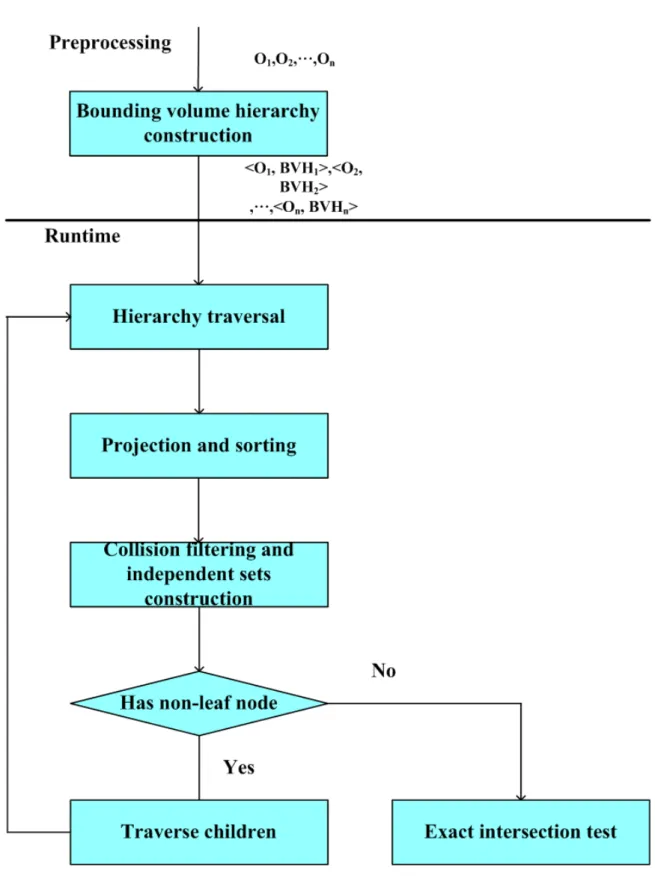
In this chapter, we present a framework for the proposed collision filtering system. The framework consists of construction of the bounding volume hierarchies, projection and depth sorting, visibility pruning collision filtering with depth sorting, and collision inde-pendent sets construction using the hierarchical structure, as shown in Figure 3.1.

In preprocessing, we construct a bounding volume hierarchy in a top-down manner for each object using oriented bounding boxes. This bounding volume hierarchy describes an object at various levels of detail. During runtime, we perform hierarchy traversal for col-lision filtering. The bounding volumes of objects are projected on the view direction, and sorted in a near-to-far order. Such sorted order is used in visibility pruning and enhances the performance of CULLIDE in the cause of collision filtering. During hierarchical prun-ing, we can select different view direction at each level for collision filtering and construct multiple collision independent sets which will greatly reduce the pairwise computation and the times of occlusion query and rendering. Finally, the exact intersection test among po-tentially colliding triangles are performed on the CPU.

As stated before, the performance of CULLIDE is restricted by the extent of projection overlapping along the view, and the resulting single potentially colliding set implies a

(29)

3.1 Overview 17

(30)

3.2 Collision filtering with depth order 18 tential large number of collision detections. For simplicity reson, in this chapter, we first introduce the collision filtering based on depth order, then incorporate collision indepen-dent sets construction into the collision filtering process. Finally, the hierarchical traversal for collision filtering is presented.

3.2 Collision filtering with depth order

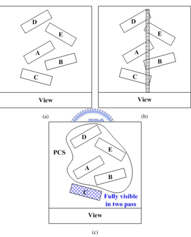
The visibility-based collision filtering in CULLIDE analyses the projection of objects from 3D to 2D image using rasterization of graphics hardware. It is quite often that objects are disjoint in 3D space, but can not be claimed disjoint by CULLIDE, due to the projections could overlap with each other. As shown in Figure 3.2, all five objects are disjoint, but only object C can be excluded from the resulting potentially colliding set.

In order to amend the performance of visibility pruning in CULLIDE, we render objects in an order sorted by depth. The axis-aligned bounding box of each object is projected onto the view direction. Two extreme, M axi and M ini, of the projection of object Oi, for all

objects, are sorted. In general, a sort would take O(n · log n), where n is the number of objects. However, under the assumption of slow motion, temporal coherence can be applied. In addition to sorting, we need to keep track of the changes in overlap status of interval pairs. By doing so, the time complexity of the sorting will be reduced to O(n + ε), where ε is the number of exchanges in the list [CLMP95]. Figure 3.3 is a result of projection and sorting.

Using hardware supported, occlusion queries, we can obtain how many pixels are ren-dered on the frame buffer [GRLM03]. and judge whether an object is fully visible with re-spect to the previously rendered objects. As in CULLIDE, fully visible objects are pruned in two passes from potentially colliding set. We decide a rendering order as O₁0, O₂0, . . ., O0_n, and let M ini > M inj, where i < j. To avoid the problem described in Figure 3.2,

objects are rendered from far to near far-to-near in the first pass.

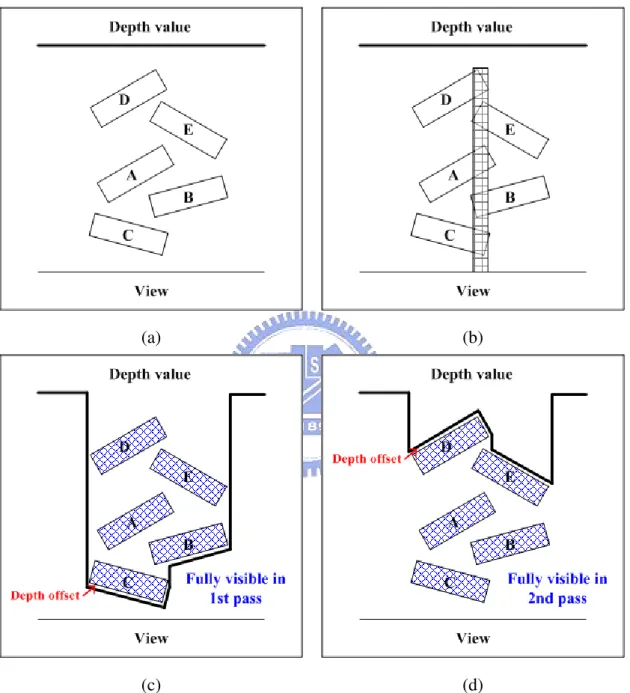
In the second pass, if objects are rendered in a near-to-far order, farer objects might be occluded by nearer ones. Instead, we move the view from z-near to z-far and render objects in a far-to-near order. In addition, we offset a tolerance distance to depth value in two passes, to make sure that the depth values of all pixels in the first pass are closer than depth values in the second pass. The depth buffer clearing is only performed once during collision pruning. Our algorithm is shown in Algorithm 3.1. Figure 3.4 shows a result of

(31)

3.2 Collision filtering with depth order 19

(a) (b)

(c)

Figure 3.2: The worst case of CULLIDE: (a) It shows that there are no intersections in the environment; (b) All the projections of objects overlap with each other; (C) We only can prune the object C using visibility-based pruning in CULLIDE.

(32)

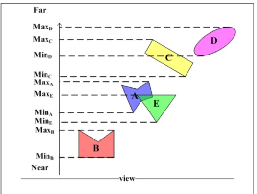
3.3 Collision Independent Sets Construction Using Separating Surfaces 20

Figure 3.3: Projection and sorting. our collision filtering with depth order.

3.3 Collision Independent Sets Construction Using

Sepa-rating Surfaces

CULLIDE prunes away objects that do not collide with any object in the final PCS. Concep-tually, for each pruned object, there is a separating surface between it and the PCS. Such a concept can be extended to partition the PCS into several collision independent sets, which are sets of objects satisfying the property that any pair of objects from two different sets will not collide. A separating surface partitions a set of objects into two nonempty subsets, placed at opposite side of the surface, as shown in Figure 3.5.

If a set S is a collision independent set, then it will not collide with any other objects, as shown in Figure 3.6(a). To determine whether S is a collision independent set, we perform the visibility test for the objects that are not in S. When all of these objects are fully visible with respect to S, we can conclude that objects in S do not collide with these objects, and hence S is a collision independent set. In the following, two lemmas are given. Lemma 1 implies that the visibility test is not required when S and O do not overlap along the

(33)

3.3 Collision Independent Sets Construction Using Separating Surfaces 21 Algorithm 3.1: Our collision culling algorithm

//1st_pass;

ClearBuf f er( DEPTH ); DepthOf f set( -ε );

foreach object Oiin a far-to-near orderdo

DepthMask( FALSE ); DepthFunc( GEQUAL ); RerderUsingOcclusionQuery( Oi); DepthMask( TRUE ); DepthFunc( LESS ); Rerder( Oi); end foreach object Oido GetQuery( Oi); end //2nd_pass; DepthOffset( +ε );

foreach object Oiin a near-to-far orderdo

if IsV isibleIn1st( Oi) == truethen

DepthMask( FALSE ); DepthFunc( LEQUAL );

RerderUsingOcclusionQuery( Oi );

end

if IsInvisibleIn1st( Oi ) == truethen

DepthMask( TRUE ); DepthFunc( GREATER ); Rerder( Oi ); end end foreach object Oi do GetQuery( Oi);

if IsV isibleInT woP asses( Oi ) == truethen

RemoveFromPCS( Oi );

end end

(34)

(a) (b)

(c) (d)

Figure 3.4: The result of our collision culling: (a) It shows that there are no intersections in the environment; (b) All the projections of objects overlap with each other; (c),(d) There are no occlusion in two passes.

(35)

Figure 3.5: If S1 and S2 do not collide with each other, we can find a separating surface

among them. viewing direction.

Lemma 1. If a set of objects S and an object O do not overlap along the viewing direction, then there exists a separating surface between S andO.

Proof: By separating axis theorem, if projections of two objects do not overlap along a direction, then two objects do not collide with each other. Besides this, we can find a surface which separates these two objects. By the same way, if projections of a set of objects S and an object O do not overlap along the viewing direction, then any object in S and O do not collide with each other. Therefore, we can find a surface separating S and O. Lemma 2. If a set of objects S and an object O overlap along a direction, but O is fully visible with respect toS, then there exists a separating surface between S and O.

Proof: It have been proven in [GRLM03] that there are no intersections between an object O and a set S, if Oiis fully visible with respect to S. Though the projections of O and S

overlap along a direction, we will still find a separating surface between them.

In determining if S in Figure 3.6 is a collision independent set, by Lemma 1., O2 and

(36)

(a) (b)

Figure 3.6: (a) Collision independent set; (b) The projection of green objects overlap with the collision independent set, and the projection of yellow objects dose not overlap with the set.

all of the green objects are fully visible with respect to S, then S is a collision independent set. If any of the green objects is not fully visible, then we insert the object into S.

In the first pass, we reduce objects in far-to-near order based on the minimum depth M ini of object Oi. If an object is fully visible, it is discarded; otherwise, it is the first

element of a newly created collision independent set. Once a collision independent set S is constructed. We continue to render the objects that are overlapped with S along the view direction. We discard the one that is fully visible and insert to the S the one that is not fully visible. Note that once such an insertion occur, we need a way to indicate which objects are overlapped with the new S. After all the objects overlapped with S are rendered, we continue to render the remaining objects and search for the next object is not fully visible and construct the next collision independent set. After the first pass, we guarantee there is no overlapping among the interval of the projection of potential collision independent sets along the view direction. Furthermore, we indicate the separating surfaces at the nearest part of potential collision independent sets.

Collision independent sets constructed in the first pass generally are not complete. Those objects that are fully visible with respect to the previously rendered object may collide with objects in some collision independent sets. In the second pass, we move the view from near to far an render those objects in far-to-near order, and insert each object that is not fully visible to an appropriate collision independent set. Such a independent set

(37)

3.3 Collision Independent Sets Construction Using Separating Surfaces 25 can be found in constant time by using separating surface indicated in the first pass.

In order to perform the collision independent sets construction in linear time, we expect to have one visibility test for each object in the first pass. We propose a method for updating the overlapping region with respective to the collision independent set under construction. We design a probing surface pointing to the minimum depth of objects that are overlapped with the object to be rendered. Probing surface will be assigned to overlapping region once an object becomes the first object in a newly created collision independent set or is inserted into a collision independent set.

Since we construct collision independent sets on the 1D view direction, if two collision independent sets overlap along the view direction then we can not distinguish them. In section 3.4, we will apply the algorithm to a hierarchical structure, and replace single view direction with multiple view directions to reduce this limitation.

Regard Figure 3.7 as the example. The visibility test of objects of O5, O8, O3, O4, O2,

O6, O1, and O7 are performed in the first pass. We disregard O5 due to it is fully visible.

O8 is non-fully visible, we construct a collision independent set CIS1and insert O8into it

set. The only overlapped object with CIS1 is O3 and O3 is fully visible, we can confirm

that CIS1 will not collide with any objects that are not yet rendered. Similarly, CIS2

containing O4 is constructed since O4 is not fully visible, and the overlapped object O2 is

fully visible. CIS2 also dose not collide with remaining objects. After CIS3 containing

O6 is constructed, we do visibility test for the overlapped objects O1 and O7. Only O7 is

not fully visible, and inserted into CIS3. Separating surfaces SS1, SS2, and SS3 point

to the minimum depth of CIS3, CIS2, and CIS1, respectively. In the second pass, we

only perform visibility test for O1, O2, O3, and O5, since these objects are fully visible

in first pass. O2, O3, and O5 are not fully visible, and inserted into CIS3, CIS2, and

CIS1, respectively. As a result of three collision independent sets P CS1 = {O5, O8},

P CS2 = {O3, O4}, and P CS3 = {O2, O6, O7} are constructed.

Some symbols are described before we introduce the proposed algorithms. Eiis a temp

for traversing all projection elements in the sorted list. In each iteration, Ei scans the list

from far to near in the first pass and then from near to far in the second pass. ActiveCIS is used to indicate the collision independent set that is being constructed. SS is a separating surface. It will separate the ActiveCIS from other collision independent sets. P S is a probing surface pointing to the minimum depth of objects that are overlapped with the

(38)

(39)

3.3 Collision Independent Sets Construction Using Separating Surfaces 27 Table 3.1: Parameters of collision independent sets construction

Notation Description

Ei each sorted element after projection

ActiveCIS the constructing collision independent set SS the potential separating surface

OV overlapping region corresponding to ActiveCIS P S probing surface for updating overlapped region

object to be rendered. OV is a depth indicating the overlapping region of ActiveCIS. P S will be assigned to OV once an object becomes the first object in a newly created collision independent set of is inserted into ActiveCIS. The algorithm of collision independent sets construction is shown in Algorithm 3.2.

3.3.1 First Pass in Collision Culling

P S is set to positive infinity initially. We traverse all projection elements from far to near and construct collision independent sets. If Ei points the maximum depth of an object Oi

and P S is greater than the minimum depth of Oi, then we update P S to the minimum depth

of Oi. If Eiis a minimum value of Oi, then Oiis performed visibility test. If Oi is not fully

visible,we check whether the ActiveCIS exists. If ActiveCIS is nil, then we construct a new collision independent set, represented by ActiveCIS; otherwise we insert Oiinto ActiveCIS,

and update separating surface SS and overlapping region OV . The separating surface SS points to the minimum value of Oi showing that there might be a separating surface pass

through it. OV points to the position of probing surface P S.

After Oiperformed visibility test, if the ActiveCIS exists (ActiveCIS 6= nil) and Eipoint

to a overlapping region OV , then we can make sure that there is a separating surface passing through SS and separating ActiveCIS and other untested objects. We record the ActiveCIS and SS into a list of collision independent set, and set ActiveCIS to nil. This means that there is no potentially colliding set expanding.

(40)

3.3.2 Second Pass in Collision Culling

In the second pass, we detect objects that belong to the collision independent sets con-structed in the first pass. It is completed in linear time using the separating surfaces which are derived in the first pass. These separating surfaces will avoid ambiguous situations and ensure that each potentially colliding object will be inserted into correct collision indepen-dent set. We scan projection elements from near to far. If Eiis a minimum value of Oi, then

we check whether Oiis fully visible in the first pass. If the object is not fully visible in the

first pass and Ei points to separating surface SS, then we assign the collision independent

set corresponding to SS to ActiveCIS. If the object is fully visible in the first pass, then we perform visibility test for it, and insert it into ActiveCIS if the object is non-fully visible in the second pass.

3.3.3 A detailed process of collision independent sets construction

An example is shown in Figure 3.8, traverse the projection elements: e5, e8, e3, b5, b8, e4,

b3, e2, b4, e1, e6, b2, e7, b6, b1, and b7, where ei and bi are the farthest and nearest part of

Oi with respect to the view direction, respectively. Objects of O5, O8, O3, O4, O2, O6, O1,

and O7 are performed visibility test in the first pass.

In Figure 3.9, we sequentially traverse projection elements of e5, e8, and e3. e5, e8, and

e3are farthest part of objects, and probing surface P S is updated to b3, the nearest position

of O5, O8, and O3. P S records the conservative overlapping region with respect to e3.

b5 and b8 are traversed, and O5 and O8 are performed visibility test in order. Only O8

is non-fully visible, and then we construct a potentially collision independent set CIS1,

insert O8 into the set and assign CIS1 to ActiveCIS. The separating surface SS1 and

overlapping region OV1point to b8and P S, respectively. This means that there may exist a

separation surface between CIS1and untested objects. The result is shown in Figure 3.10.

If all untested objects are fully visible before OV1, then CIS1is a collision independent set

and there is a separating surface pass through b3.

e4 and b3 are traversed in order, P S is updated to b4and O3 is performed visibility test.

O3 is fully visible and P S1 points to b3. This means all overlapped objects with respect to

CIS1 are fully visible, and CIS1will not collide with any objects that nearer than SS1. we

(41)

3.4 Collision filtering in hierarchical structure 29 We traverse e2and b4in order, update P S to b2and perform visibility test for O4. CIS2

is constructed and assigned to ActiveCIS due to O4 is non-fully visible and ActiveCIS

is nil. SS2 and OV2 with respect to CIS2 point to b2 and P S, respectively, as shown in

Figure 3.12. A new collision independent set is found at O4, and OV2is indicated by P S.

e1, e6 and b2 are traversed in order, P S is updated to b1 and O2 is performed visibility

test. The expansion of CIS2 is finished due to O2 is fully visible and OV2 points to b2,

and we remove CIS2from ActiveCIS, as shown in Figure 3.13. O2is an only overlapped

object with CIS2, and it is fully visible. This means CIS2dose not collide any objects that

nearer than SS2.

We traverse e7and b6in order, update P S to b7and perform visibility test for O6. CIS3

is constructed and assigned to ActiveCIS due to O6 is non-fully visible and ActiveCIS

is nil. SS3 and OV3 with respect to CIS3 point to b6 and P S, respectively, as shown in

Figure 3.14. b1and b7are traversed, and we perform visibility test with O1and O7in order.

Only O7 is non-fully visible and ActiveCIS is not nil, then we insert O7 into CIS3. The

result of the example in the first pass is shown in Figure 3.15. There are three collision independent sets P CS1 = {O8}, P CS2 = {O4}, and P CS3 = {O6, O7} found.

In the second pass, we traverse the projection elements in near-to-far order, and perform visibility test for objects of O1, O2, O3, and O5 which are fully visible in first pass. O2,

O3, and O5 are non-fully visible, and inserted into CIS3, CIS2, and CIS1, respectively.

There are three collision independent sets P CS1 = {O5, O8}, P CS2 = {O3, O4}, and

P CS3 = {O2, O6, O7}, and two separating surfaces are found among collision independent

sets. The result is shown in Figure 3.16. .

3.4 Collision filtering in hierarchical structure

3.4.1 Bounding Volume Hierarchy Construction

The construction of bounding volume hierarchy can be done in either top-down, bottom-up, or incremental fashion. In order to build a complete tree and group neighboring primitives, we use top-down construction. Collision culling will be processed in a coarse to fine man-ner by traversing the bounding volume hierarchy which will substantially reduce the time required for visibility queries [BM04]. This should be handled by broad phase collision

(42)

3.4 Collision filtering in hierarchical structure 30

Figure 3.8: An example, a scene consists of O1, O2, O3, O4, O5, O6, O7, and O8.

Figure 3.9: Traverse projection elements of e5, e9, and e3. The global probing surface P Sg

(43)

Figure 3.10: Traverse projection elements of b5 and b8, collision independent set CIS1 is

constructed at O8.

Figure 3.11: Traverse projection elements of e4and b3, and the expansion of CIS1 is finish

(44)

Figure 3.12: Traverse projection elements of e2 and b4, collision independent set CIS2 is

constructed at O4.

Figure 3.13: Traverse projection elements of e1, e6 and b2, and the expansion of CIS2 is

(45)

Figure 3.14: Traverse projection elements of e7 and b6, collision independent set CIS3 is

constructed at O6.

Figure 3.15: After the first pass, three independent colliding sets, P CS1 = {O8}, P CS2 =

(46)

Figure 3.16: After the second pass, the three collision independent sets will be finalized as CIS1 = {O5, O8}, CIS2 = {O3, O4}, and CIS3 = {O2, O6, O7}, and there are two

(47)

3.4 Collision filtering in hierarchical structure 35 Algorithm 3.2: The algorithm of collision independent sets construction

//1st_pass;

ActiveCIS = nil, OV = nil, CISList = {}, P S = ∞; foreach element Eiin a far-to-near orderdo

if Ei == MAX andP S > GetM in( Ei )then

P S = GetM in( Ei );

else if Ei== MINthen

VisibilityTest( Ei);

if IsInvisible( Ei) == truethen

if ActiveP CS = nil then

ConstructCIS( ActiveCIS ); end InsertIntoCIS( Oi, ActiveCIS ); SS = Ei; OV = P S; end

if ActiveP CS 6= nil and OV = Eithen

Complete( ActiveCIS, SS, CISList ); ActiveP CS = nil;

end end

if ActivePCS 6= nil then

Complete( ActiveCIS, SS ); end

//2ndpass;

foreach element Ei in a near-to-far orderdo

if Ei == MINthen

if IsInvisibleIn1st( Ei) == true and SSExists(Ei )then

ActiveCIS = GetCIS( Ei, CISList );

else if IsVisibleIn1st( Ei) == truethen

V isibilityT est( Ei);

if IsInvisible( Ei ) == truethen

InsertIntoCIS( Oi, ActiveCIS );

end end

(48)

Figure 3.17: Bounding volume hierarchy with a 8-ary tree.

detection. But bounding volume hierarchy is mainly for narrow phase collision detection. Since a frame buffer clearing is called for each level of hierarchy, we replace the original binary trees for bounding volume hierarchy by the 8-ary trees to decrease the height of a tree, as shown in Figure 3.17. Moreover, we offset boundary of volumes by a small distance to avoid collisions missing due to insufficient frame buffer resolution in collision culling. 3.4.1.1 Bounding Volume Hierarchy Optimization

In this section, we will present how to construct oriented bounding boxes. The covariance matrix provides a measure of the correlation among the vertices in a set. The direction and density of the vertex distribution can be described using the eigenvalues and eigenvec-tors of the covariance matrix. The covariance matrix [Cij] of vertices of an object can be

represented by Cjk = n X i=1 Ai 12AH(9c i jc i k+ p i jp i k+ q i jq i k+ r i jr i k) − c H j c H k

Let vertices pi, qi, and riare the three vertices of the i’th triangle. where Ai = 1 2|(p

i_{− q}i_{) ×}

(pi− ri_{)| and A}H ₌Pn

j A

j _{representing the area of triangle i and the summed area of all}

triangles, respectively, ci _{= (p}i_{+ q}i _{+ r}i_{)/3 and c}H ₌ PiAi·ci

AH representing the centroid of triangle i and all triangles, respectively. The three eigenvectors of the covariance matrix

(49)

(a) (b)

Figure 3.18: Bounding volume hierarchy construction using (a) three eigenvectors of the covariance matrix; (b) optimizing principal components

can be used as the three axes of the oriented bounding box. This, however, is not optimal. One improved approach, called optimizing principal components [Eri05], is to first align the box along one of the eigenvectors, and then determine two remaining eigenvectors by using the computed minimum-are bounding rectangle of the projection of vertices onto the plane perpendicular to the first axis. This method determines the best orientation of two remaining axes and produces the smallest volume oriented bounding box. Figure 3.18 shows the bounding volume hierarchy constructed using 3 eigenvectors of the covariance matrix and optimizing principal components, respectively.

3.4.2 Sorting and collision independent sets construction

In subsection 3.3, we present an approach to partition potentially colliding set into multiple subsets. We project axis-aligned bounding volumes of objects and find the separating sur-faces along the view direction. However, if the intervals of the projections of two collision independent sets overlap along the view direction, these sets might be unable to distinguish. For this reason, we attempt to apply the proposed algorithm to a hierarchical structure.

During hierarchy traversal, we select the different view directions for performing col-lision culling for each level. The axis-aligned bounding volumes of remaining objects are rearrange along the view direction, and the projection elements are also scanned from far to near and then from near to far. For each independent set, we maintain an additional sorted

(50)

3.4 Collision filtering in hierarchical structure 38 list for the projections of objects of the set, because we only consider the overlapping region in the same independent set, and the subsets are computed in each collision independent set. In this way, collision independent sets will be constructed more efficiently, we can reduce the influence of that the projections of collision independent sets overlap on the specific direction. Moreover, the first tested object of each collision independent set need not carry out visibility test, and the last tested object of each collision independent set need not update to the depth buffer.

(51)

C H A P T E R

4

Results

We have implemented the proposed algorithm in C++ and OpenGL, and compare the per-formance of the algorithm with CULLIDE [GRLM03] on VC 7.0 with 3.0GHz Intel Pen-tium 4 CPU, 512 MB memory, and Geforce 6800 GPU. Three different scenes of vary-ing benchmarks are tested. The dynamic computation is supported by the physics engine Tokama.

Since bounding volume hierarchy is part of the proposed approach and it is beneficial to the objects of high geometry complexity, performances of CULLIDE (called CULLIDE-w/o-BVH), CULLIDE with bounding bolume hierarchy (called CULLIDE with BVH), and our approach are compared by collision detection time. We also implement CULLIDE-w/o-BVH in two stages, object level and sub-object level. For each level, we choose +x-axis, −x-+x-axis, +y-+x-axis, −y-+x-axis, +z-+x-axis, and −z-axis to regard as view direction. After potentially colliding set computation, potentially colliding pairs are determined by using sweep-and-prune algorithm, and exact intersections of potentially colliding pairs are com-puted on CPU eventually. For possible optimaizations in CULLIDE, we perform off-screen rendering by using frame buffer object such that the resolution of testing buffer will not be restricted to window size. Testing on hight resolution can be done using frame buffer object with cost lower than pbuffer. Additionally, we use vertex array object to place geometry of a model on the video memory beforehand to avoid a large number of geometric data transferring between CPU and GPU. In the experiments, two timing statistics are recorded.

(52)

4.1 Performance analysis in simple environment 40 The first is the average collision detection time, defined as

Average CD time = Pn

i=1CD timei

n

where n is the number of frames performed and CD timei is the collision detection time

in i’th frame. The second is the maximum collision detection time M aximum CD time = max

i {CD timei}.

If the maximum collision detection time is too large, that means the algorithm will not detect collisions efficiently when there are many intersections, and we can not calculate the cost of detecting collision in prediction.

4.1 Performance analysis in simple environment

Environment 1 is a scene of lower geometry and depth complexity, consisting of 50 torii and 2 planes. Each torus consists of 800 triangles, and each plane consists of 1800 triangles. All the torii move with gravity but two planes are fixed.

We perform physics simulation at 500-1200 frame buffer resolutions. We repeatedly simulate 10 times for each frame buffer resolution over a period of time, and some of the simulating process are shown in Figure 4.1. Timing statistics of simulation results are shown in Table 4.1 and Figure 4.2. It is shown that the average collision detection time is around 4-6 milliseconds and the maximum collision detection time is lower than 30 mil-liseconds in our approach. In CULLIDE-w/o-BVH and CULLIDE with BVH, the average collision detection time is around 9-12 and 7-10 millisecond and the maximum collision detection time is around 34-45 and 29-33 milliseconds, respectively. Our approach is about two times faster then CULLIDE-w/o-BVH.

Figure 4.3 depicts the collision detection time of the simulation over a short period of time. Figure 4.4 shows that the number of collision independent set corresponding to the same time period in Figure 4.3.

(53)

4.1 Performance analysis in simple environment 41

(a) (b)

(c) (d)

(e) (f)

(54)

(a) Average collision time.

(b) Maximum collision time.

Figure 4.2: Performance comparison between our approach and CULLIDE in environment 1.

(55)

Figure 4.3: Performance comparison with CULLIDE, CULLIDE with hierarcical bounding volume, and our approach in environment 1 at frame buffer resolution 800×800.

(56)

Figure 4.4: The number of collision independent sets constructed for environment 1 at frame buffer resolution 800×800.

(57)

4.2 Performance comparison for environments of high geometry complexity and low depth complexity 45 Resolution 500 600 700 800 900 1000 1100 1200 CULLIDE 10.4387 9.4688 11.2566 11.9801 12.3607 10.4257 12.1255 11.2271 CULLIDE + BVH 8.2661 7.7312 8.8909 9.5789 10.0679 8.2891 9.6388 8.927 Our approach 4.984 4.3461 5.258 6.4132 6.1873 4.8549 5.7734 5.186

(a)The average collision time (in ms).

Resolution 500 600 700 800 900 1000 1100 1200 CULLIDE 43.6992 35.9532 39.3979 41.0256 45.1085 34.0662 39.4205 37.6131 CULLIDE + BVH 32.9125 29.1949 29.6336 32.4783 34.6623 27.8242 31.967 28.9488 Our approach 27.8145 21.5791 21.9499 25.8569 28.2488 21.3527 22.5531 21.0549

(b)The maximum collision time (in ms). Table 4.1: Timing statistics for environment 1.

4.2 Performance comparison for environments of high

ge-ometry complexity and low depth complexity

Environment 2 is a scene of high geometry complexity that consists of 12 dragons and two planes. Each dragon and plane are composed of 47794 and 1800 triangles, respectively. Environment setting is the same as environment 1, all the dragons are affected with gravity, and two planes are fixed. Collision responses between dragons and between dragons and the fixed planes are decided by the physics engine. Some of simulation process is shown in Figure 4.5. Table 4.2 shows the timing statistics of simulation at frame buffer resolutions of 500-1200. From Figure 4.6, we can see that there is a large difference on collision detection time between CULLIDE-w/o-BVH and CULLIDE with BVH. The maximum collision time of our approach is slower than CULLIDE with BVH at some resolutions, because the number of collision independent set is 1 and the construction of collision independent set brings additional overhead. However, the average performance of our approach is faster than CULLIDE with BVH.

From the simulation result, we observe that hierarchical bounding volumes can actually improve the performance. Figures 4.7 and 4.8 show the performance of our method and CULLIDE with BVH, we can see that the difference of performance is reduced. It suggests that hierarchical bounding volume is advantageous to the scene of high geometry complex-ity since the times of visibilcomplex-ity queries will be reduced substantially by using the bounding volume hierarchy. In Figure 4.9, we observe that only a few collision independent sets are

(58)

4.2 Performance comparison for environments of high geometry complexity and low depth complexity 46

(a) (b)

(c) (d)

(e) (f)

(59)

4.2 Performance comparison for environments of high geometry complexity and low depth complexity 47

(a) Average collision time.

(b) Maximum collision time.

Figure 4.6: Performance comparison between our approach and CULLIDE in environment 2.

複雜環境之影像式碰撞濾除運算

國

立

交

通

大

學

資訊科學與工程研究所

碩

士

論

文

複雜環境之影像式碰撞濾除運算

A Practical Collision Filtering for Complex Environments

Using Image-based Techniques

研 究 生：陳勇誠

指導教授：莊榮宏 教授

複雜環境之影像式碰撞濾除運算

A Practical Collision Filtering for Complex Environments Using

Image-based Techniques

研 究 生：陳勇誠 Student：Yong-Cheng Chen

指導教授：莊榮宏 Advisor：Jung-Hong Chuang

國 立 交 通 大 學

資 訊 科 學 與 工 程 研 究 所

碩 士 論 文

複雜環境之影像式碰撞濾除運算

學生： 陳勇誠 指導教授: 莊榮宏 博士

國立交通大學資訊工程學系

摘要

A Practical Collision Filtering for Complex Environments

using Image-based Techniques

Student: Yong-Cheng Chen

Advisor: Dr. Jung-Hong Chuang

Department of Computer Science and Information Engineering

National Chiao Tung University

ABSTRACT

Contents

List of Figures

List of Algorithms

List of Tables

Acknowledgments

C H A P T E R

1

Introduction

1.1

Collision Detection

1.2

Collision Detection Algorithms

1.3

Motivation

1.4

Organization

C H A P T E R

2

Related Work

2.1

Ray Casting

2.2

Counting Boundary Crossings

2.3

Layered Depth Images

2.4

Collision Culling

C H A P T E R

3

Image-based Collision

Filtering

3.1

Overview

3.2

Collision filtering with depth order

3.3

Collision Independent Sets Construction Using

Sepa-rating Surfaces

3.3.1

First Pass in Collision Culling

3.3.2

Second Pass in Collision Culling

3.3.3

A detailed process of collision independent sets construction

研究生：陳勇誠

指導教授：莊榮宏教授

研究生：陳勇誠 Student：Yong-Cheng Chen

國立交通大學

資訊科學與工程研究所

碩士論文

學生：陳勇誠指導教授: 莊榮宏博士