Chapter 3. Packet Scheduling Policies
3.1 Qualcomm's Proportional Fair Algorithm
Because our packet scheduling algorithms are based on Q-PFA, we will spend
space in this section to give the details.
Q-PFA is a packet scheduling algorithm that gives every user approximately
equal air time while exploits multiuser diversity. In each slot, once the BS receives the
DRC messages, it needs two stages to do this algorithm:
Stage 1. Scheduling:
The user with the highest priority is selected, where the priority is calculated
by:
N t i
R t DRC
i
i 1,..., )
( )
Priority= ( = (3-1)
where DRCi(t) is the DRC message sent by user i at time t, Ri(t) the estimate
average rate of user i at time t, and N the number of users in that cell.
Stage 2. Update average rate:
The estimated average rate is updated by:
N i
t t T t t R
t
R i i
c i c
i 1 ( ) 1 1,...,
) 1 (
1 ) 1
( ⎟⎟× + × × =
⎠
⎜⎜ ⎞
⎝
⎛ −
=
+ (3-2)
where Ti(t) is the current transmission rate of user i. If user i was not selected
to be served, Ti(t) would be zero. 1i is an indicator function. When user i is selected at
time t, 1i equal to 1; otherwise, 1i equals 0. tc is the window size whose value is
heuristic and has an influence on how long the transmission status is remembered. If tc
is large, the estimated average rate can be more accurate. But if a user moves from a
good channel environment to a bad one and stays long in bad one, this user can be
starved. In [1], [4], [6] and [10], the value of tc is assumed to be 1000 slots.
To show how Q-PFA can exploit multiuser diversity, we now use a simple
example to explain it. Let us consider two different cases where both cases have two
users and the window size is 10. In case 1, the channel condition is fixed. User A has
the rate of 100 and user B has the rate of 10. In case 2, the channel condition varies
with time. The rate of user A fluctuates between 80 and 120, and the rate of user B
fluctuates between 8 and 12, as shown in Figure 3-1. The rate would not change
during a slot. We see that case-2 users are in the unfavorable conditions that they not
only start at low rate but also two thirds of the slots are at low rate.
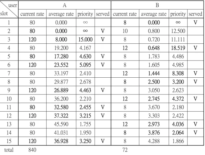
Now, we apply Q-PFA to both cases. The results are shown in Table 3-1 and
to add more users under the situation that the channel condition is fixed. It can be
observed that Q-PFA is identical to round-robin when channel state is fixed..
Figure 3-1. The bold lines show the rate of case 1; the dashed lines show the rate of case 2.
In case 2, we can find that after the second slot, if a user is at its relatively good
channel condition, this user will be selected. Thus, although the average channel
conditions of case-2 users are worse than that of case-1 user, the overall throughput in
case 2 is higher.
From this example, one can easily realize that Q-PFA is suitable for scheduling
service in time-varying channel environment. For an environment like Ethernet that
the channel state is almost fixed, Q-PFA has no advantage over round-robin.
Furthermore, if we can estimate the average rate correctly, we can then choose the
“right” user to serve. This is due to the fact that how Q-PFA determines which user to
choose depends on the current rate (i.e. the DRC messages) and the estimated average
rate. We can not change the current rate using a packet scheduling algorithm, but the
average rate is what we are going to estimate.
A B
user
slot current rate average rate priority served current rate average rate priority served
1 100 0.000 ∞ V 10 0.000 ∞
2 100 10.000 10.000 10 0.000 ∞ V
3 100 9.000 11.111 V 10 1.000 10.000
4 100 18.100 5.525 10 0.900 11.111 V
5 100 16.290 6.139 V 10 1.810 5.525
6 100 24.661 4.055 10 1.629 6.139 V
7 100 22.195 4.506 V 10 2.466 4.055
8 100 29.975 3.336 10 2.219 4.506 V
9 100 26.978 3.707 V 10 2.998 3.336
10 100 34.280 2.917 10 2.698 3.707 V
11 100 30.852 3.241 V 10 3.428 2.917
12 100 37.767 2.648 10 3.085 3.241 V
13 100 33.990 2.942 V 10 3.777 2.648
14 100 40.591 2.464 10 3.399 2.942 V
15 100 36.532 2.737 V 10 4.059 2.464
total 800 70
Table 3-1. The result of case 1. The behavior of Q-PFA is identical to Round Robin.
A B user
slot current rate average rate priority served current rate average rate priority served
1 80 0.000 ∞ 8 0.000 ∞ V
2 80 0.000 ∞ V 10 0.800 12.500
3 120 8.000 15.000 V 8 0.720 11.111
4 80 19.200 4.167 12 0.648 18.519 V
5 80 17.280 4.630 V 8 1.783 4.486
6 120 23.552 5.095 V 8 1.605 4.985
7 80 33.197 2.410 12 1.444 8.308 V
8 80 29.877 2.678 8 2.500 3.200 V
9 120 26.889 4.463 V 8 3.050 2.623
10 80 36.200 2.210 12 2.745 4.372 V
11 80 32.580 2.455 V 8 3.670 2.180
12 120 37.322 3.215 V 8 3.303 2.422
13 80 45.590 1.755 12 2.973 4.036 V
14 80 41.031 1.950 8 3.876 2.064 V
15 120 36.928 3.250 V 8 4.288 1.866
total 840 72
Table 3-2. The result of case 2. The “right” user can usually be select to serve.
3.2 Initial Values
One problem of Q-PFA is that when a user enters the system, other users
would suffer starvation [6] of service. This is due to the fact that the estimated
average rate of the new user is zero. Thus it has the highest priority until it has been
served for some slots and the estimated average rate becomes higher.
To overcome this problem, we first noted that under Q-PFA, the users have
approximately equal air time in symmetric channel, i.e. they are served for
approximately the same number of slots. If the effective data rate of a user is R, and
the system has N users, then the estimated average data rate is about R/N. The
effective data rate of a user is the total transmitted data divided by the time used to
transmit data. (To compare, the estimated average rate is approximately the total
transmitted data divided by the total time.) We can reasonably assume that the current
rate is mostly not far from the effective data rate. So if the cell has N users and a new
user arrives, we set the initial estimated average rate, Ri(t), as:
If current_data_rate = 0 then Ri(t) = (least_data_rate)/N Else
Ri(t) = (current_data_rate)/N
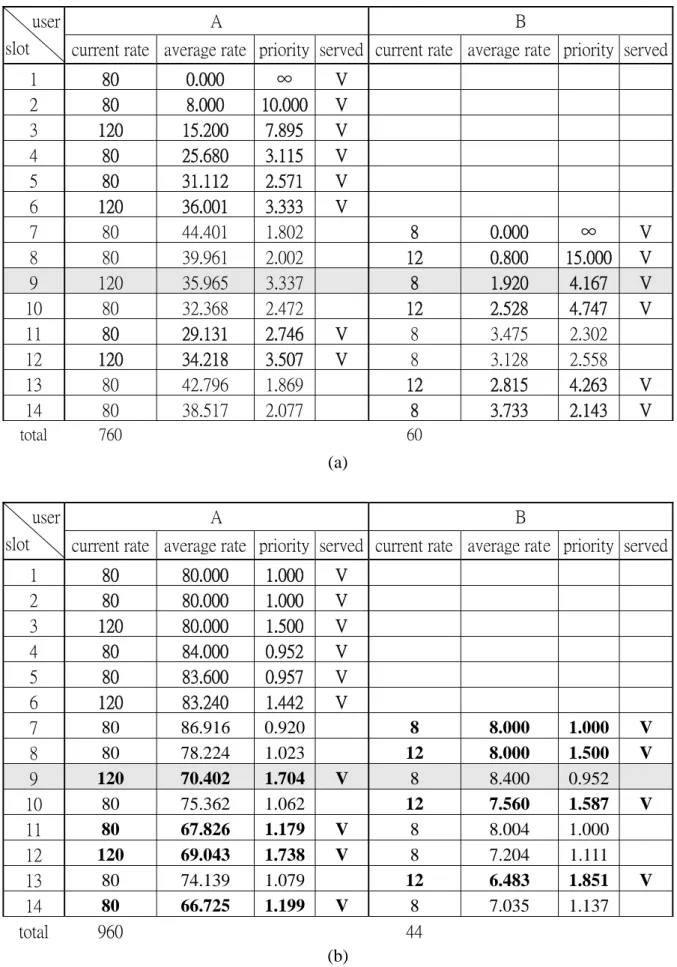
Let’s consider the case 2 example in the last section. The window size is 10,
too. But this time, user B is delayed for 6 slots (i.e. user B is a new user at 7-th slot).
As shown in Table 3-3(a), if the initial estimate is set to zero, the priority of user B
would be too high. Nearly half the window size of slots will be occupied by the new
user. At some slots, such as slot 9, the data rate of user A is relative high, but he can
not be selected for service. If we set an initial value as mentioned above, the problem
that the priority of new user is too high no longer exists, as shown in Table 3-3(b).
A B user
slot current rate average rate priority served current rate average rate priority served
1 80 0.000 ∞ V
2 80 8.000 10.000 V
3 120 15.200 7.895 V
4 80 25.680 3.115 V
5 80 31.112 2.571 V
6 120 36.001 3.333 V
7 80 44.401 1.802 8 0.000 ∞ V
8 80 39.961 2.002 12 0.800 15.000 V
9 120 35.965 3.337 8 1.920 4.167 V
10 80 32.368 2.472 12 2.528 4.747 V
11 80 29.131 2.746 V 8 3.475 2.302
12 120 34.218 3.507 V 8 3.128 2.558
13 80 42.796 1.869 12 2.815 4.263 V
14 80 38.517 2.077 8 3.733 2.143 V
total 760 60
(a)
A B
user
slot current rate average rate priority served current rate average rate priority served
1 80 80.000 1.000 V
2 80 80.000 1.000 V
3 120 80.000 1.500 V
4 80 84.000 0.952 V
5 80 83.600 0.957 V
6 120 83.240 1.442 V
7 80 86.916 0.920 8 8.000 1.000 V
8 80 78.224 1.023 12 8.000 1.500 V
9 120 70.402 1.704 V 8 8.400 0.952
10 80 75.362 1.062 12 7.560 1.587 V
11 80 67.826 1.179 V 8 8.004 1.000
12 120 69.043 1.738 V 8 7.204 1.111
13 80 74.139 1.079 12 6.483 1.851 V
14 80 66.725 1.199 V 8 7.035 1.137
total 960 44
(b)
Table 3-3. User B is a new comer at slot 7. (a) Without initial value. (b) With initial value.
3.3 Update Suspending
Consider that a user is browsing Internet. He retrieves a web page, looks at it for
a while and retrieves another page. What happen to the user’s priority if the estimated
average rate is still updated when he looks at this web page (i.e. no data to be
transmitted)? Assume tc=1000 and he looks at the page for only 3 seconds. The
estimated average rate will reduce to about 0.165 time the original value. That is, his
priority is increased to 7 times of the original priority. So we should stop updating
average rate when a user is idle.
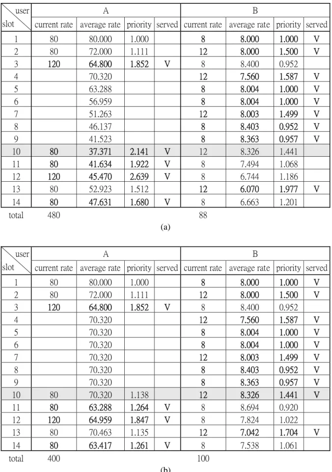
Again, let’s consider the case 2 example of section 3.1. This time, we have
applied the initial value policy, and user A will be idle from slot 4 to slot 9. As shown
in Table 3-4(a), user A continues updating the average rate. At slot 10, user A becomes
active again, he preempts user B even though user B is at his better channel state and
user A at his worse channel state. In Table 3-4(b), we stop updating during the idle
period. When user A becomes active again, user B can be selected as usual.
A B user
slot current rate average rate priority served current rate average rate priority served
1 80 80.000 1.000 8 8.000 1.000 V
2 80 72.000 1.111 12 8.000 1.500 V
3 120 64.800 1.852 V 8 8.400 0.952
4 70.320 12 7.560 1.587 V
5 63.288 8 8.004 1.000 V
6 56.959 8 8.004 1.000 V
7 51.263 12 8.003 1.499 V
8 46.137 8 8.403 0.952 V
9 41.523 8 8.363 0.957 V
10 80 37.371 2.141 V 12 8.326 1.441
11 80 41.634 1.922 V 8 7.494 1.068
12 120 45.470 2.639 V 8 6.744 1.186
13 80 52.923 1.512 12 6.070 1.977 V
14 80 47.631 1.680 V 8 6.663 1.201
total 480 88
(a)
A B
user
slot current rate average rate priority served current rate average rate priority served
1 80 80.000 1.000 8 8.000 1.000 V
2 80 72.000 1.111 12 8.000 1.500 V
3 120 64.800 1.852 V 8 8.400 0.952
4 70.320 12 7.560 1.587 V
5 70.320 8 8.004 1.000 V
6 70.320 8 8.004 1.000 V
7 70.320 12 8.003 1.499 V
8 70.320 8 8.403 0.952 V
9 70.320 8 8.363 0.957 V
10 80 70.320 1.138 12 8.326 1.441 V
11 80 63.288 1.264 V 8 8.694 0.920
12 120 64.959 1.847 V 8 7.824 1.022
13 80 70.463 1.135 12 7.042 1.704 V
14 80 63.417 1.261 V 8 7.538 1.061
total 400 100
(b)
Table 3-4. User A is idle from slot 4 to slot 9. (a) Without update suspending. (b) With update suspending.
3. 4 Active-User Monitoring
The update suspending policy prevents users from getting too high priority after
he has been idle for a period. But this raises another problem. Assume there are 10
users in a cell, who all initially have data to receive. At some moment, all of them
have become idle except user 1. The average rate of user 1 gradually gets larger as
time passes. After a while, when some of the 9 idle users want to receive data, their
estimated average rate may have been much lower then user 1. User 1 starves.
To prevent this from happening, our approach is to keep always true the
following equation in all events:
number user
active
rate data effective rate
average estimated
_ _
_ _ _
_ = . (3-3)
To achieve this goal, user i records the current active number (let it be k) when
entering the idle state. Meanwhile, other active users multiply their estimated average
rate by k/(k-1) time so as to follow equation (3-3). If user i is active again when m
active users are currently in the cell, user i's average rate is multiplied by k/(m+1) and
other user’s average rate by m/(m+1).
If we apply this policy, then a new user can be similarly treated, as a user being
from idle to busy. Thus, if we have N users in the cell, the initial value in section 3.1
should be (current data rate)/(N+1) rather than (current data rate)/N. A terminated user
should modify their average rate.
3. 5 Window Size Increasing
Before we consider another situation, let’s define the load of user i, Li, as the
estimated remaining service time of user i:
i user of rate average estimated
i user of length queue
Li
_ _ _ _ _
_ _ _
= _ . (3-4)
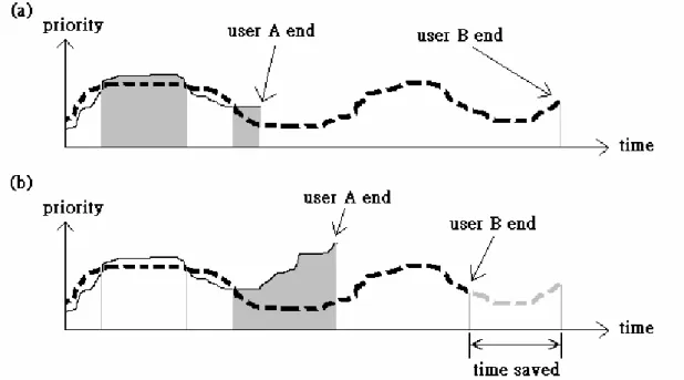
See another two-user case in Figure 3- 2(a), where user A has higher load than
user B. The shaded areas represent time periods used to serve user A and the white
areas used to serve user B. In the first shaded area of Figure 3- 2(a), the priority of
user A is slightly higher than user B. If the lower-loaded user, user A, is deferred at
this situation, he may get a chance that its priority is much higher than user B and is
selected for service, as shown in Figure 3- 2(b). Because the channel is utilized more
efficiently this way, the total needed service time can be saved.
This can happen for two reasons. First, when a user is deferred, more users are
in a cell and hence higher multiuser diversity gain is achieved. Second, if the priority
of a user is just a little higher than another, then it is reasonable that it can have even
higher priority later. Besides, a lower-loaded user usually has higher effective data
rate, which results in shorter queue more frequently. Hence, if such users are deferred,
relatively less loss will be caused.
Figure 3- 2. (a) Calculate priority and select a user to serve. (b) The lower load user is delayed.
To defer a lower-loaded user, our proposed method uses two steps:
1. Calculate the average load of a cell. Let it be Ltotal.
2. Let Li be the load of user i and 0<τ <1. If Li < τ Ltotal and user i is not selected for service, then double the windows size of user i when updating
its average rate.
If the window size of a user is doubled, then the estimated average rate reduces
slower and its priority increases slower. With this method, the priority of a
lower-loaded user will increase less rapidly, causing service deference.
After a series of steps to modify Q-PFA, if all policies are applied, the modified
Q-PFA has three stages:
Stage 0. Adjust average rate:
If a new user arrives, set the estimated average rate to (current data rate)/(N+1).
If a user becomes idle, becomes active, or leaves the system, he and other
users should change average rate as mentioned in section 3-4..
Stage 1. Scheduling:
This step is the same as the original Q-PFA.
Stage 2. Update average rate:
For user i, if Li <τ Ltotal and it is not selected to be served, then the estimated
average rate is updated by:
) 2 (
1 1 ) 1
( R t
t t
R i
c
i ⎟⎟×
⎠
⎜⎜ ⎞
⎝
⎛ −
=
+ (3-5)
else update average rate as original Q-PFA.