大規模深度圖卷積網路之快速訓練演算法

(1)

國立臺灣大學電機資訊學院資訊工程學系碩士論文

Department of Computer Science and Information Engineering College of Electrical Engineering and Computer Science

National Taiwan University Master Thesis

大規模深度圖卷積網路之快速訓練演算法

Efficient Algorithms for Training Deep and Large Graph Convolutional Networks

江韋霖 Wei-Lin Chiang

指導教授：林智仁博士 Advisors: Chih-Jen Lin, Ph.D.

中華民國 109 年 7 月 July, 2020

(2)

(3)

(4)

(5)

要

圖卷積網路 (graph convolutional networks) 是一項近年來被成功地應用在許多基於圖結構的問題上的技術，然而，要有效率地訓練大規模的圖卷積網路仍然非常具有挑戰性。在本篇論文中，我們仔細地討論了圖卷積網路的背景知識，透過點分類問題的例子介紹模型的概念，並給出其最佳化問題的數學表達式，以進行複雜度分析。在回顧完背景後，我們仔細地比較了現有的圖卷積網路訓練算法，以及其潛在的問題，大體來說，現今有許多研究者提出基於隨機梯度法的方法來解決訓練緩慢的問題，但他們仍有很高的計算成本，並且當圖卷積網路的深度加大後，其運算成本會以指數型地增長，另一方面，有些方法也在記憶體資源上的要求很高，甚至需要儲存整張圖上每個節點的嵌入向量 (embedding vector) 作為基礎，這些方法在遇到大規模的圖資料時可能會遭遇到運算資源上的瓶頸或甚至不可行。在本篇論文中，我們提出了一個快速訓練圖卷積網路的方法—聚類圖卷積網路法 (Cluster-GCN)，這個方法仍基於隨機梯度法，但充分利用了圖結構的特性來加速訓練，聚類圖卷積網路法的具體步驟如下：在預處理階段中，我們首先使用了圖聚類演算法 (graph clustering algorithm) 來將整張圖切塊成多個子圖 (subgraph)，之後在每一輪訓練時，我們隨機抽樣一個子圖的節點們，並將圖卷積網路過程中的鄰居搜索 (neighborhood search) 限制在該子圖範圍內，最後基於隨機梯度法來做模型的更新。這個簡單且有效的方法可以將記憶體資源以及計算成本大大地改善，並且也能達到跟先前方法相仿的模型正確率，在本篇論文的實驗中，我們在多個面向如：記憶體需求、訓練

(6)

時間、以及每輪的收斂速度上來檢驗不同的訓練方法，實驗結果顯示我們的算法相較於其他論文能達到幾乎最佳的表現，為了更進一步地測試該算法之擴展性 (scalability)，我們還創造了一個新的圖數據集 Amazon2M，其原始資料來自於 Amazon 購物網站上的商品分類資訊，我們利用消費者是否經常同時購買此兩產品的資訊，以圖的方式表達產品與產品之間的聯繫，具體來說形成了一個共同購買網路，該數據有 200 萬個節點以及 6100 萬條邊。實驗結果顯示我們提出的聚類圖卷積網路法在 Amazon2M 上的表現卓越，相比於先前最佳的訓練演算法我們可以達到較快的訓練速度並且使用了更少的記憶體資源，更進一步地，我們也在這篇論文中分析如何有效地訓練深度圖卷積網路，我們提出的聚類圖卷積網路法能避免掉高額的運算，並且其訓練時間以及資源成本並無增加太多，此項進展也帶來了在眾多公開數據集的突破，舉例來說：在 PPI 這個數據上，我們的算法成功訓練了一個 5 層的圖卷積網路並達到了 99.36 的 Micro-F1 正確率，相比於先前最佳的結果 98.71 還要高，顯示出我們提出的聚類圖卷積網路法能有效地訓練深度網路，而其簡單有效的特性可以作為基礎來訓練更複雜多樣的圖卷積網路法，我們也開放本算法的原始碼在 https://github.com/google-research/google-research/tree/master/

cluster_gcn 自由供公眾使用。

：圖卷積網路、大規模圖學習、深度學習

(7)

Abstract

Graph convolutional network (GCN) has been successfully applied to many graph-based applications; however, training a large-scale GCN remains challenging. In this thesis, we detailedly discuss technical background of graph convolutional networks. We begin with introducing a node classification example to motivate the problem and ideas of GCN models. Then we give mathematical notations to describe the optimization problem of GCN.

After reviewing the background, we analyze existing methods for solving large-scale GCN and discuss some possible issues in previous methods. Roughly speaking, current SG-based algorithms suffer from either a high computational cost that exponentially grows with number of GCN layers, or a large space requirement for keeping the entire graph and the embedding of each node in memory. To resolve those issues, we propose Cluster-GCN, a novel GCN algorithm that is suitable for SG-based training by exploiting the graph clustering structure. Cluster-GCN works as the following: at each step, it samples a block of nodes that associate with a dense subgraph identified by a graph clustering algorithm, and restricts the neighborhood search within this subgraph. This simple but effective strategy leads to significantly improved memory and computational efficiency while being able to achieve comparable test accuracy with previous algorithms. To demonstrate the scalability of our algorithm, we create a new Amazon2M data with 2 million nodes and 61 million edges. When training a 3-layer GCN on Amazon2M, Cluster-GCN is faster than previous state-of-the-art methods with much less

(8)

memory usage. Cluster-GCN also allows us to train much deeper GCN without much time and memory overhead, which leads to improved prediction accuracy—using a 5-layer Cluster-GCN, we achieve state-of-the-art test F1 score 99.36 on the PPI dataset, while the previous best result was 98.71.

Our codes are publicly available at https://github.com/google-research/

google-research/tree/master/cluster_gcn.

Keywords: graph convolutional networks, large-scale graph mining, deep learning

(9)

Chapter 1 Introduction

Graph convolutional network (GCN) [10] has become increasingly popular in addressing many graph-based applications, including semi-supervised node classification [10], link prediction [20] and recommender systems [18]. Given a graph, GCN uses a graph convolution operation to obtain node embeddings layer by layer—at each layer, the embedding of a node is obtained by gathering the embeddings of its neighbors, followed by one or a few layers of linear transformations and nonlinear activations. The final layer embedding is then used for some end tasks. For instance, in node classification problems, the final layer embedding is passed to a classifier to predict node labels, and thus the parameters of GCN can be trained in an end-to-end manner.

Since the graph convolution operator in GCN needs to propagate embeddings using the interaction between nodes in the graph, this makes training quite challenging. Unlike other neural networks that the training loss can be perfectly decomposed into individual terms on each sample, the loss term in GCN (e.g., classification loss on a single node) depends on a huge number of other nodes, especially when GCN goes deep. Due to the node dependence, GCN’s training is very slow and requires lots of memory – back-propagation needs to store all the embeddings in the computation graph in GPU memory.

Previous GCN Training Algorithms: To demonstrate the need of developing a scal- able GCN training algorithm, we first discuss the pros and cons of existing approaches,

(12)

in terms of 1) memory requirement¹, 2) time per epoch² and 3) convergence speed (loss reduction) per epoch. These three factors are crucial for evaluating a training algorithm.

Note that memory requirement directly restricts the scalability of algorithm, and the later two factors combined together will determine the training speed. In the following discus- sion we denote N to be the number of nodes in the graph, F the embedding dimension, and L the number of layers to analyze classic GCN training algorithms.

• Full-batch gradient descent is proposed in the first GCN paper [10]. To compute the full gradient, it requires storing all the intermediate embeddings, leading to O(N F L) memory requirement, which is not scalable. Furthermore, although the time per epoch is efficient, the convergence of gradient descent is slow since the parameters are updated only once per epoch.

[memory: bad; time per epoch: good; convergence: bad]

• Mini-batch SG is proposed in [6]. Since each update is only based on a mini- batch gradient, it can reduce the memory requirement and conduct many updates per epoch, leading to a faster convergence. However, mini-batch SG introduces a sig- nificant computational overhead due to the neighborhood expansion problem—to compute the loss on a single node at layer L, it requires that node’s neighbor nodes’

embeddings at layer L− 1, which again requires their neighbors’ embeddings at layer L− 2 and recursive ones in the downstream layers. This leads to time com- plexity exponential to the GCN depth. GraphSAGE [6] proposed to use a fixed size of neighborhood samples during back-propagation through layers and FastGCN [1]

proposed importance sampling, but the overhead of these methods is still large and will become worse when GCN goes deep.

[memory: good; time per epoch: bad; convergence: good]

• VR-GCN [2] proposes to use a variance reduction technique to reduce the size of neighborhood sampling nodes. Despite successfully reducing the size of samplings

1Here we consider the memory for storing node embeddings, which is dense and usually dominates the overall memory usage for deep GCN.

2An epoch means a complete data pass.

(13)

(in our experiments VR-GCN with only 2 samples per node works quite well), it requires storing all the intermediate embeddings of all the nodes in memory, leading to O(N F L) memory requirement. If the number of nodes in the graph increases to millions, the memory requirement for VR-GCN may be too high to fit into GPU.

[memory: bad; time per epoch: good; convergence: good.]

In this thesis, we propose a novel GCN training algorithm by exploiting the graph clustering structure. We find that the efficiency of a mini-batch algorithm can be characterized by the notion of “embedding utilization”, which is proportional to the number of links between nodes in one batch or within-batch links. This finding motivates us to design the batches using graph clustering algorithms that aims to construct partitions of nodes so that there are more graph links between nodes in the same partition than nodes in different partitions. Based on the graph clustering idea, we proposed Cluster-GCN, an algorithm to design the batches based on efficient graph clustering algorithms (e.g., METIS [9]). We take this idea further by proposing a stochastic multi-clustering framework to improve the convergence of Cluster-GCN. Our strategy leads to huge memory and computational ben- efits. In terms of memory, we only need to store the node embeddings within the current batch, which is O(bF L) with the batch size b. This is significantly better than VR-GCN and full gradient decent, and slightly better than other SG-based approaches. In terms of computational complexity, our algorithm achieves the same time cost per epoch with gradient descent and is much faster than neighborhood searching approaches. In terms of the convergence speed, our algorithm is competitive with other SG-based approaches. Fi- nally, our algorithm is simple to implement since we only compute matrix multiplication and no neighborhood sampling is needed. Therefore for Cluster-GCN, we have [memory:

good; time per epoch: good; convergence: good].

We conducted comprehensive experiments on several large-scale graph datasets and made the following contributions:

• Cluster-GCN achieves the best memory usage on large-scale graphs, especially on deep GCN. For example, Cluster-GCN uses 5x less memory than VRGCN in a 3- layer GCN model on Amazon2M. Amazon2M is a new graph dataset that we con-

(14)

struct to demonstrate the scalablity of the GCN algorithms. This dataset contains a amazon product co-purchase graph with more than 2 millions nodes and 61 millions edges.

• Cluster-GCN achieves a similar training speed with VR-GCN for shallow networks (e.g., 2 layers) but can be faster than VR-GCN when the network goes deeper (e.g., 4 layers), since our complexity is linear to the number of layers L while VR-GCN’s complexity is exponential to L.

• Cluster-GCN is able to train a very deep network that has a large embedding size.

Although several previous works show that deep GCN does not give better performance, we found that with proper optimization, deeper GCN could help the accuracy. For example, with a 5-layer GCN, we obtain a new benchmark accuracy 99.36 for PPI dataset, comparing with the highest reported one 98.71 by [19].

Implementation of our proposed method is publicly available.³ The rest of the thesis is organized as follows. In Chapter 2, we review the background of GCN and discuss its challenges in terms of memory and computation bottlenecks. We then propose a cluster- GCN algorithm in Chapter 3 to resolve these issues and present the experimental results in Chapter 4.⁴ We conclude the thesis in Chapter 5.

3https://github.com/google-research/google-research/tree/master/cluster_gcn

4Note that Chapters 3 and 4 are based on our earlier paper [3]

(15)

Chapter 2 Background of GCN

In this chapter we discuss technical background of graph convolutional networks. We begin with introducing a toy example to motivate the research problem and ideas of GCN models. Then we give mathematical notations to describe the optimization problem of GCN. Later we review existing methods for solving large-scale GCN and discuss some possible issues in their methods.

2.1 A Toy Example

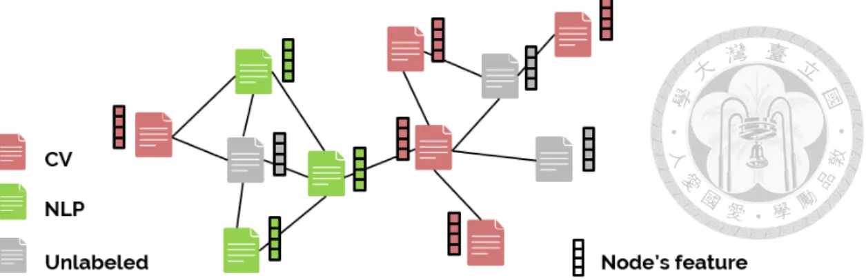
We begin with an example of node classification on a citation networks shown in Fig- ure 2.1, where each node corresponds to a paper and each edge represents the citation relationship between papers. In this example, some paper nodes are labelled with their topics (e.g., CV or NLP) and we assume feature vectors describing contents of papers (e.g., term frequency) are given. Our goal is to design a model that utilizes the above information to predict categories of unlabelled paper nodes. Unlike some traditional machine learning tasks where only features and labels are involved, node classification on graph brings more complexity to the problem as relations between data points need to be properly handled to make better predictions. That is, we not only learn a mapping from the feature space to the label space but also hope to better utilize those given relations between existing data points. For example, a citation relationship between two papers could be an indication that their topics are somewhat related. The idea of GCN is to obtain bet-

(16)

Figure 2.1: A toy example of node classification on a citation networks.

ter representation vectors that integrate original feature vectors with their neighborhood information. The resulting representation vectors can then be useful for downstream tasks like node classification, graph classification and also link prediction.

2.2 Notations

Now we formally introduce mathematical notations of node classification problems. Sup- pose we are given a graph G = (V, E, A), which consists of N = |V| vertices and |E|

edges such that an edge between any two vertices i and j represents their similarity. The corresponding adjacency matrix A is an N × N sparse matrix, where

A_ij =









1 if there is an edge between i and j, 0 otherwise.

Also, each node is associated with an F -dimensional feature vector x_iand a K-dimemsional vector y_i, where K is the number of classes considered in the classification problem. In a multi-class setting, if the node i is in class k then

y_i = [0, . . . , 0

| {z }

k−1

, 1, 0, . . . , 0]^T ∈ R^K.

On the other hand, in a multi-label setting, more than one entry in y_i may have the value 1. We denote the feature matrix X ∈ R^N^×F and the label matrix Y ∈ R^N^×K for all N

(17)

1 2

3 4

Figure 2.2: A 4-node graph.

nodes.

2.3 The Idea of GCN

A GCN layer aims to obtain better node representations by incorporating neighboring embedding vectors and multiply them with a weighted matrix W⁽ⁱ⁾ to generate output vectors. A L-layer GCN repeats the procedure L times as follows.

X⁽⁰⁾ = X −−−−−→^{GCN Layer}

A,W⁽⁰⁾

X⁽¹⁾· · · X^(L−1) GCN Layer−−−−−−→

A,W^(L⁻¹⁾

X^(L),

where X^(L)is the final representation vectors we desire to obtain. A vanilla GCN layer [10]

considers averaging all embedding vectors in the neighborhood. For example, if we con- sider an example of four nodes in Figure 2.2, Node-1’s new embedding x⁽¹⁾₁ is obtained by

x⁽¹⁾₁ = σ(W⁽⁰⁾mean(x⁽⁰⁾₁ , x⁽⁰⁾₂ , x⁽⁰⁾₃ , x⁽⁰⁾₄ )),

where σ(·) is an activation function such as RELU and W⁽⁰⁾ ∈ R^F⁰^×F¹ is a weighted matrix. Similarly, other nodes’ embeddings are updated by

x⁽¹⁾₂ = σ(W⁽⁰⁾mean(x⁽⁰⁾₂ , x⁽⁰⁾₁ )), x⁽¹⁾₃ = σ(W⁽⁰⁾mean(x⁽⁰⁾₃ , x⁽⁰⁾₁ )), x⁽¹⁾₄ = σ(W⁽⁰⁾mean(x⁽⁰⁾₄ , x⁽⁰⁾₁ )).

This procedue helps to integrate neighborhood information into each node’s embedding.

When a L-layer GCN is considered, the final representation vector of a node will incor- porate information of its L-hop neighborhood (i.e., nodes reachable by≤ L steps).

(18)

In fact, if we construct a normalized adjacency matrix

A^′ = D⁻¹A,

where D is diagonal with Dii = ∑N

j=1Aij, a GCN layer can be then represented in a matrix form

Z^(l+1) = A^′X^(l)W^(l), X^(l+1)= σ(Z^(l+1)), (2.1)

where W^(l) ∈ R^F^l^×F^l+1 is the feature transformation matrix which will be learned for the downstream tasks. Note that for simplicity we assume the feature dimensions are the same for all layers (F₁ =· · · = FL= F ).

When using GCN for node classification, the goal is to learn weight matrices in (2.1) by minimizing the following objective with a loss function ξ(·):

L = 1 N

∑N i=1

ξ(y_i, z^(L)_i ), (2.2)

where z^(L)_i is the i-th row of Z^(L)indicating the final layer prediction of node i, and y_i is the ground-truth label. In practice, a cross-entropy loss is commonly used for node classification in multi-class or multi-label problems.

2.4 Challenges in Large-scale GCNs

In this section, we discuss why solving a large-scale GCN can be difficult. The first no- table difference between GCN and other common networks (e.g., fully connected nets, convolutional nets) is that the loss associated with each data point depends not only on its input feature x⁽⁰⁾_i but all its neighboring embeddings. To see the difference, we take CNN as an example. We know a CNN maps one image to one label vector so its optimization problem can be decomposed as

min

θ

1 N

∑N i=1

ξ(y_i, CNN_θ(z⁽⁰⁾_i )),

(19)

where θ is the collection of all weight matrices in the CNN model and

ξ_i = ξ(y_i, CNN_θ(z⁽⁰⁾_i ))

solely relies on z⁽⁰⁾_i . However, we cannot conduct the same point-level decomposition for GCN because the final output z^(L)_i may depend on other input feature vectors. For example, in Figure 2.2, the new embedding of node-1 is

z⁽¹⁾₁ = σ(W⁽⁰⁾mean(z⁽⁰⁾₁ , z⁽⁰⁾₂ , z⁽⁰⁾₃ , z⁽⁰⁾₄ )).

Hence training a large GCN becomes challenging because of the following reasons.

1. Calculating full gradient can be prohibitively expensive

2. Stochastic gradients (SG) methods can not be directly applied as the loss function is not decomposable

3. An implementation for handling large graphs is not trivial

We take the previous example in Figure 2.3 to demonstrate why calculating subsampled gradient over some instances is not trivial. Suppose a 2-layer GCN is used and we desire to calculate the loss and gradient associated with the target node 1 (like taking batch size

= 1). To obtain its loss and gradient, we need to calculate its final representation z⁽²⁾₁ , which further requires all node embeddings in its 2-hop neighborhood. That is, we need to access all neighbors’ neighbors of the target node (the yellow circle). The calculation looks like a recursive process

z⁽²⁾₁ = σ(W⁽¹⁾mean(z⁽¹⁾₁ , z⁽¹⁾₂ , z⁽¹⁾₃ , z⁽¹⁾₄ )),

where

z⁽¹⁾₁ = σ(W⁽⁰⁾mean(z⁽⁰⁾₁ , z⁽⁰⁾₂ , z⁽⁰⁾₃ , z⁽⁰⁾₄ )) z⁽¹⁾₂ = σ(W⁽⁰⁾mean(z⁽⁰⁾₁ , z⁽⁰⁾₂ , z⁽⁰⁾₅ ))

...

(20)

Figure 2.3: 2-hop neighborhood of the target node.

There are some potential issues when conducting such a procedure

1. Frequent indexing: the loss and gradient evaluation involves the indexing of neighboring nodes, making the implementation complicated

2. Low embedding utilization: in this case, 10 nodes’ embeddings are considered but we only get one z⁽²⁾₁

3. Neighborhood explosion: the size of neighbors can grow exponentially as the number of GCN layers increases

In fact, the above issues occur when a small number of nodes is selected. We will explain more details in the next section.

2.5 Issues of Existing Methods

In this section, we discuss issues of some existing methods and detailedly analyze their time and memory complexity.

In the original GCN paper [10], full gradient descent is used to train GCN, but it suffers from high computational and memory cost. In terms of memory, computing the full gradient of (2.2) by back-propagation requires storing all the embedding matrices{Z^(l)}^Ll=1

which needs O(N F L) space. In terms of the convergence speed, since the model is only updated once per epoch, the training requires more epochs to converge.

(21)

It has been shown that mini-batch SG can improve the training speed and memory requirement of GCN in some recent works [6, 1, 2]. Instead of computing the full gradient, SG only needs to calculate the gradient based on a mini-batch for each update. in this thesis, we useB ⊆ [N] with size b = |B| to denote a batch of node indices, and each SG step will compute the gradient estimation

1

|B|

∑

i∈B

∇ξ(yi, z^(L)_i ) (2.3)

to perform an update. Despite faster convergence in terms of epochs, SG will introduce another computational overhead on GCN training (as explained in the previous section), which makes it having much slower per-epoch time compared with full gradient descent.

Why does vanilla mini-batch SG have slow per-epoch time? We consider the com- putation of the gradient associated with one node i : ∇ξ(yi, z^(L)_i ). Clearly, this requires the embedding of node i, which depends on its neighbors’ embeddings in the previous layer. To fetch each node i’s neighbor nodes’ embeddings, we need to further aggregate each neighbor node’s neighbor nodes’ embeddings as well. Suppose a GCN has L + 1 layers and each node has an average degree of d, to get the gradient for node i, we need to aggregate features from O(d^L) nodes in the graph for one node. That is, we need to fetch information for a node’s hop-k (k = 1,· · · , L) neighbors in the graph to perform one update. Computing each embedding requires O(F²) time due to the multiplication with W^(l), so in average computing the gradient associated with one node requires O(d^LF²) time.

Embedding utilization can reflect computational efficiency. If a batch has more than one node, the time complexity is less straightforward since different nodes can have overlapped hop-k neighbors, and the number of embedding computation can be less than the worst case O(bd^L). To reflect the computational efficiency of mini-batch SG, we de- fine the concept of “embedding utilization” to characterize the computational efficiency.

During the algorithm, if the node i’s embedding at l-th layer z^(l)_i is computed and is reused u times for the embedding computations at layer l + 1, then we say the embedding utiliza-

(22)

tion of z^(l)_i is u. For mini-batch SG with random sampling, u is very small since the graph is usually large and sparse. Assume u is a small constant (almost no overlaps between hop-k neighbors), then mini-batch SG needs to compute O(bd^L) embeddings per batch, which leads to O(bd^LF²) time per update and O(N d^LF²) time per epoch.

We illustrate the neighborhood expansion problem in the left panel of Fig. 2.4. On the contrary, full-batch gradient descent has the maximal embedding utilization—each embedding will be reused d (average degree) times in the upper layer. As a consequence, the original full gradient descent [10] only needs to compute O(N L) embeddings per epoch, which means on average only O(L) embedding computation is needed to acquire the gradient of one node.

To make mini-batch SG work, previous approaches try to restrict the neighborhood expansion size, which however do not improve embedding utilization. GraphSAGE [6]

uniformly samples a fixed-size set of neighbors, instead of using a full-neighborhood set.

We denote the sample size as r. This leads to O(r^L) embedding computations for each loss term but also makes gradient estimation less accurate. FastGCN [1] proposed an important sampling strategy to improve the gradient estimation. VR-GCN [2] proposed a strategy to store the previous computed embeddings for all the N nodes and L layers and reuse them for unsampled neighbors. Despite the high memory usage for storing all the N L embeddings, we find their strategy very useful and in practice, even for a small r (e.g., 2) can lead to good convergence.

We summarize the time and space complexity in Table 2.1. Clearly, all the SG-based algorithms suffer from exponential complexity with respect to the number of layers, and for VR-GCN, even though r can be small, they incur huge space complexity that could go beyond a GPU’s memory capacity. In Chapter 3, we introduce our Cluster-GCN algorithm, which achieves the best of two worlds—the same time complexity per epoch with full gradient descent and the same memory complexity with vanilla SG.

(23)

Table 2.1: Time and space complexity of GCN training algorithms. L is number of layers, N is number of nodes, ∥A∥0 is number of nonzeros in the adjacency matrix, and F is number of features. For simplicity we assume number of features is fixed for all layers.

For SG-based approaches, b is the batch size and r is the number of sampled neighbors per node. Note that due to the variance reduction technique, VR-GCN can work with a smaller r than GraphSAGE and FastGCN. For memory complexity, LF²is for storing{W^(l)}^Ll=1

and the other term is for storing embeddings. For simplicity we omit the memory for storing the graph (GCN) or sub-graphs (other approaches) since they are fixed and usually not the main bottleneck.

Time Complexity Memory Complexity GCN [10] O(L∥A∥0F + LN F²) O(LN F + LF²)

Vanilla SG O(d^LN F²) O(bd^LF + LF²)

GraphSAGE [6] O(r^LN F²) O(br^LF + LF²)

FastGCN [1] O(rLN F²) O(brLF + LF²)

VR-GCN [2] O(L∥A∥0F + LN F² + r^LN F²) O(LN F + LF²) Cluster-GCN O(L∥A∥0F + LN F²) O(bLF + LF²)

Figure 2.4: The neighborhood expansion difference between traditional graph convolution and our proposed cluster approach in Chapter 3. The red node is the starting node for neighborhood nodes expansion. Traditional graph convolution suffers from exponential neighborhood expansion, while our method can avoid expensive neighborhood expansion.

(24)

(25)

Chapter 3 Proposed Method

3.1 Vanilla Cluster-GCN

Our Cluster-GCN technique is motivated by the following question: In mini-batch SG updates, can we design a batch and the corresponding computation subgraph to maximize the embedding utilization? We answer this affirmative by connecting the concept of embedding utilization to a clustering objective.

Consider the case that in each batch we compute the embeddings for a set of nodesB from layer 1 to L. Since the same subgraph A_B,B (links withinB) is used for each layer of computation, we can then see that embedding utilization is the number of edges within this batch∥AB,B∥0. Therefore, to maximize embedding utilization, we should design a batchB to maximize the within-batch edges, by which we connect the efficiency of SG updates with graph clustering algorithms.

Now we formally introduce Cluster-GCN. For a graph G, we partition its nodes into c groups: V = [V1,· · · Vc] whereVt consists of the nodes in the t-th partition. Thus we have c subgraphs as

G = [G¯ ₁,· · · , Gc] = [{V1,E1}, · · · , {Vc,Ec}],

where eachEt only consists of the links between nodes inVt. After reorganizing nodes,

(26)

the adjacency matrix is partitioned into c² submatrices as

A = ¯A + ∆ =







A₁₁ · · · A1c

... . .. ... A_c1 · · · Acc





 (3.1)

and

A =¯







A11 · · · 0 ... . .. ... 0 · · · Acc





, ∆ =







0 · · · A1c

... . .. ... A_c1 · · · 0





, (3.2)

where each diagonal block A_ttis a|Vt|×|Vt| adjacency matrix containing the links within G_t. ¯A is the adjacency matrix for graph ¯G; A_st contains the links between two partitions Vsand Vt; ∆ is the matrix consisting of all off-diagonal blocks of A. Similarly, we can partition the feature matrix X and training labels Y according to the partition [V1,· · · , Vc] as [X1,· · · , Xc] and [Y1,· · · , Yc] where Xtand Ytconsist of the features and labels for the nodes in V_trespectively.

The benefit of this block-diagonal approximation ¯G is that the objective function of GCN becomes decomposible into different batches (clusters). Let ¯A^′denotes the normalized version of ¯A, the final embedding matrix becomes

Z^(L)= ¯A^′σ( ¯A^′σ(· · · σ( ¯A^′XW⁽⁰⁾)W⁽¹⁾)· · · )W^(L⁻¹⁾ (3.3)

=







A¯^′₁₁σ( ¯A^′₁₁σ(· · · σ( ¯A^′₁₁X₁W⁽⁰⁾)W⁽¹⁾)· · · )W^(L⁻¹⁾ ...

A¯^′_ccσ( ¯A^′_ccσ(· · · σ( ¯A^′_ccX_cW⁽⁰⁾)W⁽¹⁾)· · · )W^(L⁻¹⁾







due to the block-diagonal form of ¯A (note that ¯A^′_ttis the corresponding diagonal block of A¯^′). The loss function can also be decomposed into

LA^¯^′ =∑

t

|Vt|

N LA^¯^′_tt and LA^¯^′_tt = 1

|Vt|

∑

i∈Vt

ξ(y_i, z^(L)_i ). (3.4)

The Cluster-GCN is then based on the decomposition form in (3.3) and (3.4). At each

(27)

step, we sample a clusterVtand then conduct SG to update based on the gradient ofLA^¯^′_tt, and this only requires the sub-graph A_tt, the X_t, Y_t on the current batch and the models {W^(l)}^Ll=1. The implementation only requires forward and backward propagation of matrix products (one block of (3.3)) that is much easier to implement than the neighborhood search procedure used in previous SG-based training methods.

We use graph clustering algorithms to partition the graph. Graph clustering methods such as Metis [9] and Graclus [5] aim to construct the partitions over the vertices in the graph such that within-clusters links are much more than between-cluster links to better capture the clustering and community structure of the graph. These are exactly what we need because: 1) As mentioned before, the embedding utilization is equivalent to the within-cluster links for each batch. Intuitively, each node and its neighbors are usually located in the same cluster, therefore after a few hops, neighborhood nodes with a high chance are still in the same cluster. 2) Since we replace A by its block diagonal approxima- tion ¯A and the error is proportional to between-cluster links ∆, we need to find a partition to minimize number of between-cluster links.

In Figure 2.4, we illustrate the neighborhood expansion with full graph G and the graph with clustering partition ¯G. We can see that cluster-GCN can avoid heavy neighborhood search and focus on the neighbors within each cluster. In Table 3.1, we show two different node partition strategies: random partition versus clustering partition. We partition the graph into 10 parts by using random partition and METIS. Then use one partition as a batch to perform a SG update. We can see that with the same number of epochs, using clustering partition can achieve higher accuracy. This shows using graph clustering is important and partitions should not be formed randomly.

Time and space complexity. Since each node inVtonly links to nodes insideVt, each node does not need to perform neighborhoods searching outside A_tt. The computation for each batch will purely be matrix products ¯A^′_ttX_t^(l)W^(l)and some element-wise operations, so the overall time complexity per batch is O(∥Att∥0F + bF²). Thus the overall time complexity per epoch becomes O(∥A∥0F + N F²). In average, each batch only requires computing O(bL) embeddings, which is linear instead of exponential to L. In terms of

(28)

Table 3.1: Random partition versus clustering partition of the graph (trained on mini-batch SG). Clustering partition leads to better performance (in terms of test F1 score) since it removes less between-partition links. These three datasetes are all public GCN datasets.

We will explain PPI data in the experiment part. Cora has 2,708 nodes and 13,264 edges, and Pubmed has 19,717 nodes and 108,365 edges.

Dataset random partition clustering partition

Cora 78.4 82.5

Pubmed 78.9 79.9

PPI 68.1 92.9

space complexity, in each batch, we only need to load b samples and store their embed- dings on each layer, resulting in O(bLF ) memory for storing embeddings. Therefore our algorithm is also more memory efficient than all the previous algorithms. Moreover, our algorithm only requires loading a subgraph into GPU memory instead of the full graph (though graph is usually not the memory bottleneck). The detailed time and memory complexity are summarized in Table 2.1.

3.2 Stochastic Multiple Partitions

Although vanilla Cluster-GCN achieves good computational and memory complexity, there are still two potential issues:

• After the graph is partitioned, some links (the ∆ part in Eq. (3.1)) are removed.

Thus the performance could be affected.

• Graph clustering algorithms tend to bring similar nodes together. Hence the distribution of a cluster could be different from the original data set, leading to a biased estimation of the full gradient while performing SG updates.

In Figure 3.1, we demonstrate an example of unbalanced label distribution by using the Reddit data with clusters formed by Metis. We calculate the entropy value of each cluster based on its label distribution. Comparing with random partitioning, we clearly see that entropy of most clusters are smaller, indicating that the label distributions of clusters are biased towards some specific labels. This increases the variance across different batches and may affect the convergence of SG.

(29)

Figure 3.1: Histograms of entropy values based on the label distribution. Here we present within each batch using random partition versus clustering partition. Most clustering partitioned batches have low label entropy, indicating skewed label distribution within each batch. In comparison, random partition will lead to larger label entropy within a batch although it is less efficient as discussed earlier. We partition the Reddit dataset with 300 clusters in this example.

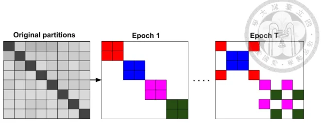
To address the above issues, we propose a stochastic multiple clustering approach to incorporate between-cluster links and reduce variance across batches. We first partition the graph into p clustersV1,· · · , Vpwith a relatively large p. When constructing a batch B for an SG update, instead of considering only one cluster, we randomly choose q clusters, denoted as t1, . . . , tqand include their nodes{Vt1∪· · ·∪Vtq} into the batch. Furthermore, the links between the chosen clusters,

{Aij | i, j ∈ t1, . . . , t_q},

are added back. In this way, those between-cluster links are re-incorporated and the combinations of clusters make the variance across batches smaller. Figure 3.2 illustrates our algorithm—for each epochs, different combinations of clusters are chosen as a batch. We conduct an experiment on Reddit to demonstrate the effectiveness of the proposed approach. In Figure 3.3, we can observe that using multiple clusters as one batch could improve the convergence. Our final Cluster-GCN algorithm is presented in Algorithm 1.

(30)

Figure 3.2: The proposed stochastic multiple partitions scheme. In each epoch, we ran- domly sample q clusters (q = 2 is used in this example) and their between-cluster links to form a new batch. Same color blocks are in the same batch.

Figure 3.3: Comparisons of choosing one cluster versus multiple clusters. The former uses 300 partitions. The latter uses 1500 and randomly select 5 to form one batch. We present epoch (x-axis) versus F1 score (y-axis).

(31)

Algorithm 1: Cluster GCN

Input: Graph A, feature X, label Y ; Output: Node representation ¯X

1 Partition graph nodes into c clustersV1,V2,· · · , Vcby METIS;

2 for iter = 1,· · · , max_iter do

3 Randomly choose q clusters, t₁,· · · , tqfromV without replacement;

4 Form the subgraph ¯G with nodes ¯V = [Vt1,Vt2,· · · , Vtq] and links AV, ¯¯V ;

5 Compute g← ∇LAV, ¯¯V (loss on the subgraph AV, ¯¯V) ;

6 Conduct Adam update using gradient estimator g

7 Output: {Wl}^Ll=1

3.3 Issues of Training Deeper GCNs

Previous attempts of training deeper GCNs [10] seem to suggest that adding more layers is not helpful. However, the datasets used in the experiments may be too small to make a proper justification. For example, [10] considered a graph with only a few hundreds of training nodes for which overfitting can be an issue. Moreover, we observe that the optimization of deep GCN models becomes difficult as it may impede the information from the first few layers being passed through. In [10], they adopt a technique similar to residual connections [7] to enable the model to carry the information from a previous layer to a next layer. Specifically, they modify (2.1) to add the hidden representations of layer l into the next layer.

X^(l+1) = σ(A^′X^(l)W^(l)) + X^(l) (3.5)

Here we propose another simple technique to improve the training of deep GCNs. In the original GCN settings, each node aggregates the representation of its neighbors from the previous layer. However, under the setting of deep GCNs, the strategy may not be suitable as it does not take the number of layers into account. Intuitively, neighbors nearby should contribute more than distant nodes. We thus propose a technique to better address this issue. The idea is to amplify the diagonal parts of the adjacency matrix A used in each GCN layer. In this way, we are putting more weights on the representation from the previous layer in the aggregation of each GCN layer. An example is to add an identity to

(32)

A as follows.¯

X^(l+1) = σ((A^′+ I)X^(l)W^(l)) (3.6)

While (3.6) seems to be reasonable, using the same weight for all the nodes regardless of their numbers of neighbors may not be suitable. Moreover, it may suffer from numerical instability as values can grow exponentially when more layers are used. Hence we propose a modified version of (3.6) to better maintain the neighborhoods information and numerical ranges. We first add an identity to the original A and perform the normalization

A = (D + I)˜ ⁻¹(A + I), (3.7)

and then consider

X^(l+1) = σ(( ˜A + λdiag( ˜A))X^(l)W^(l)). (3.8)

Experimental results of adopting the “diagonal enhancement” techniques are presented in Section 4.4 where we show that this new normalization strategy can help to build deep GCN and achieve SOTA performance.

(33)

Chapter 4 Experiments and Results

4.1 Experiment Settings

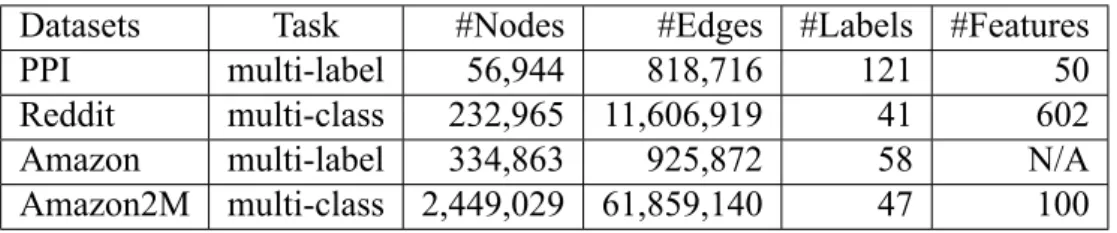
We evaluate our proposed method for training GCN on two tasks: multi-label and multi- class classification on four public datasets. The statistic of the data sets are shown in Table 4.1. Note that the Reddit dataset is the largest public dataset we have seen so far for GCN, and the Amazon2M dataset is collected by ourselves and is much larger than Reddit (see more details in Section 4.3).

We include the following state-of-the-art GCN training algorithms in our comparisons:

• Cluster-GCN (Our proposed algorithm): the proposed fast GCN training method.

• VRGCN¹ [2]: It maintains the historical embedding of all the nodes in the graph and expands to only a few neighbors to speedup training. The number of sampled neighbors is set to be 2 as suggested in [2]².

1GitHub link: https://github.com/thu-ml/stochastic_gcn

2Note that we also tried the default sample size 20 in VRGCN package but it performs much worse than sample size= 2.

Table 4.1: Data statistics

Datasets Task #Nodes #Edges #Labels #Features

PPI multi-label 56,944 818,716 121 50

Reddit multi-class 232,965 11,606,919 41 602

Amazon multi-label 334,863 925,872 58 N/A

Amazon2M multi-class 2,449,029 61,859,140 47 100

(34)

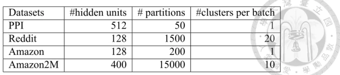
Table 4.2: The parameters used in the experiments.

Datasets #hidden units # partitions #clusters per batch

PPI 512 50 1

Reddit 128 1500 20

Amazon 128 200 1

Amazon2M 400 15000 10

• GraphSAGE³ [6]: It samples a fixed number of neighbors per node. We use the default settings of sampled sizes for each layer (S₁ = 25, S₂ = 10) in GraphSAGE.

We implement our method in PyTorch [15]. For the other methods, we use all the original papers’ code from their github pages. Since [10] has difficulty to scale to large graphs, we do not compare with it here. Also as shown in [2] that VRGCN is faster than FastGCN, so we do not compare with FastGCN here. For all the methods we use the Adam optimizer with learning rate as 0.01, dropout rate as 20%, weight decay as zero. The mean aggregator proposed by [6] is adopted and the number of hidden units is the same for all methods.

Note that techniques such as (3.8) is not considered here. In each experiment, we consider the same GCN architecture for all methods. For VRGCN and GraphSAGE, we follow the settings provided by the original papers and set the batch sizes as 512. For Cluster-GCN, the number of partitions and clusters per batch for each dataset are listed in Table 4.2.

Note that clustering is seen as a preprocessing step and its running time is not taken into account in training. In Section 6.1, we show that graph clustering only takes a small portion of preprocessing time. All the experiments are conducted on a machine with a NVIDIA Tesla V100 GPU (16 GB memory), 20-core Intel Xeon CPU (2.20 GHz), and 192 GB of RAM.

4.2 Training Performance for Median Size Datasets

Training Time vs Accuracy: First we compare our proposed method with other methods in terms of training speed. In Figure 4.2, the x-axis shows the training time in seconds, and y-axis shows the accuracy (F1 score) on the validation sets. We plot the training time

3GitHub link: https://github.com/williamleif/GraphSAGE

(35)

Table 4.3: Comparisons of memory usages on different datasets. Numbers in the brackets indicate the size of hidden units used in the model.

2-layer 3-layer 4-layer

VRGCN Cluster-GCN GraphSAGE VRGCN Cluster-GCN GraphSAGE VRGCN Cluster-GCN GraphSAGE

PPI (512) 258 MB 39 MB 51 MB 373 MB 46 MB 71 MB 522 MB 55 MB 85 MB

Reddit (128) 259 MB 284 MB 1074 MB 372 MB 285 MB 1075 MB 515 MB 285 MB 1076 MB Reddit (512) 1031 MB 292 MB 1099 MB 1491 MB 300 MB 1115 MB 2064 MB 308 MB 1131 MB

Amazon (128) 1188 MB 703 MB N/A 1351 MB 704 MB N/A 1515 MB 705 MB N/A

Table 4.4: Benchmarking on the Sparse Tensor operations in PyTorch and TensorFlow.

A network with two linear layers is used and the timing includes forward and backward operations. Numbers in the brackets indicate the size of hidden units in the first layer.

Amazon data is used.

PyTorch TensorFlow Avg. time per epoch (128) 8.81s 2.53s Avg. time per epoch (512) 45.08s 7.13s

versus accuracy for three datasets with 2,3,4 layers of GCN. Since GraphSAGE is slower than VRGCN and our method, the curves for GraphSAGE only appear for PPI and Reddit datasets. We can see that our method is the fastest for both PPI and Reddit datasets for GCNs with different numbers of layers.

For Amazon data, since nodes’ features are not available, an identity matrix is used as the feature matrix X. Under this setting, the shape of parameter matrix W⁽⁰⁾ becomes 334863x128. Therefore, the computation is dominated by sparse matrix operations such as AW⁽⁰⁾. Our method is still faster than VRGCN for 3-layer case, but slower for 2- layer and 4-layer ones. The reason may come from the speed of sparse matrix operations from different frameworks. VRGCN is implemented in TensorFlow, while Cluster-GCN is implemented in PyTorch whose sparse tensor support are still in its very early stage. In Table 4.4, we show the time for TensorFlow and PyTorch to do forward/backward operations on Amazon data, and a simple two-layer network are used for benchmarking both frameworks. We can clearly see that TensorFlow is faster than PyTorch. The difference is more significant when the number of hidden units increases. This may explain why Cluster-GCN has longer training time in Amazon dataset.

Memory usage comparison: For training large-scale GCNs, besides training time, memory usage needed for training is often more important and will directly restrict the scalability. The memory usage includes the memory needed for training the GCN for

(36)

Table 4.5: The most common categories in Amazon2M.

Categories number of products

Books 668,950

CDs & Vinyl 172,199 Toys & Games 158,771

many epochs. As discussed in Section 2.5, to speedup training, VRGCN needs to save historical embeddings during training, so it needs much more memory for training than Cluster-GCN. GraphSAGE also has higher memory requirement than Cluster-GCN due to the exponential neighborhood growing problem. In Table 4.3, we compare our memory usage with VRGCN’s memory usage for GCN with different layers. When increasing the number of layers, Cluster-GCN’s memory usage does not increase a lot. The reason is that when increasing one layer, the extra variable introduced is the weight matrix W^(L), which is relatively small comparing to the sub-graph and node features. While VRGCN needs to save each layer’s history embeddings, and the embeddings are usually dense and will soon dominate the memory usage. We can see from Table 4.3 that Cluster-GCN is much more memory efficient than VRGCN. For instance, on Reddit data to train a 4-layer GCN with hidden dimension to be 512, VRGCN needs 2064MB memory, while Cluster-GCN only uses 308MB memory.

4.3 Experimental Results on Amazon2M

A new GCN dataset: Amazon2M. By far the largest public data for testing GCN is Reddit dataset with the statistics shown in Table 4.1, which contains about 200K nodes. As shown in Figure 4.2 GCN training on this data can be finished within a few hundreds seconds. To test the scalability of GCN training algorithms, we constructed a much larger graph with over 2 millions of nodes and 61 million edges based on Amazon co-purchasing networks [14, 13]. The raw co-purchase data is from Amazon-3M⁴. In the graph, each node is a product, and the graph link represents whether two products are purchased together. Each node feature is generated by extracting bag-of-word features from the product descriptions

4http://manikvarma.org/downloads/XC/XMLRepository.html

(37)

Table 4.6: Comparisons of running time, memory and testing accuracy (F1 score) for Amazon2M.

Time Memory Test F1 score

VRGCN Cluster-GCN VRGCN Cluster-GCN VRGCN Cluster-GCN

Amazon2M (2-layer) 337s 1223s 7476 MB 2228 MB 89.03 89.00

Amazon2M (3-layer) 1961s 1523s 11218 MB 2235 MB 90.21 90.21

Amazon2M (4-layer) N/A 2289s OOM 2241 MB N/A 90.41

followed by Principal Component Analysis [8] to reduce the dimension to be 100. In addition, we use the top-level categories as the labels for that product/node (see Table 4.5 for the most common categories). The detailed statistics of the data set are listed in Table 4.1.

In Table 4.6, we compare with VRGCN for GCNs with a different number of layers in terms of training time, memory usage, and test accuracy (F1 score). As can be seen from the table that 1) VRGCN is faster than Cluster-GCN with 2-layer GCN but slower than Cluster-GCN when increasing one layer while achieving similar accuracy. 2) In terms of memory usage, VRGCN is using much more memory than Cluster-GCN (5 times more for 3-layer case), and it is running out of memory when training 4-layer GCN, while Cluster- GCN does not need much additional memory when increasing the number of layers, and achieves the best accuracy for this data when training a 4-layer GCN.

4.4 Training Deeper GCNs

In this section we consider GCNs with more layers. We first show the timing comparisons of Cluster-GCN and VRGCN in Table 4.7. PPI is used for benchmarking and we run 200 epochs for both methods. We observe that the running time of VRGCN grows exponentially because of its expensive neighborhood finding, while the running time of Cluster-GCN only grows linearly.

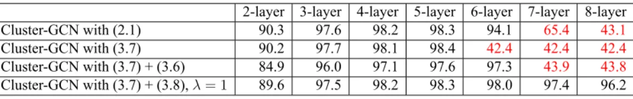
Next we investigate whether using deeper GCNs obtains better accuracy. In Sec- tion 4.4, we discuss different strategies of modifying the adjacency matrix A to facilitate the training of deep GCNs. We apply the diagonal enhancement techniques to deep GCNs and run experiments on PPI. Results are shown in Table 4.9. For the case of 2 to 5 lay-

(38)

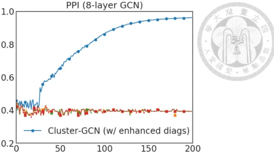
Figure 4.1: Convergence figure on a 8-layer GCN. We present numbers of epochs (x- axis) versus validation accuracy (y-axis). All methods except for the one using (3.8) fail to converge.

ers, the accuracy of all methods increases with more layers added, suggesting that deeper GCNs may be useful. However, when 7 or 8 GCN layers are used, the first three methods fail to converge within 200 epochs and get a dramatic loss of accuracy. A possible reason is that the optimization for deeper GCNs becomes more difficult. We show a detailed convergence of a 8-layer GCN in Figure 4.1. With the proposed diagonal enhancement technique (3.8), the convergence can be improved significantly and similar accuracy can be achieved.

State-of-the-art results by training deeper GCNs. With the design of Cluster- GCN and the proposed normalization approach, we now have the ability for training much deeper GCNs to achieve better accuracy (F1 score). We compare the testing accuracy with other existing methods in Table 4.8. For PPI, Cluster-GCN can achieve the state-of-art result by training a 5-layer GCN with 2048 hidden units. For Reddit, a 4-layer GCN with 128 hidden units is used.

(39)

Table 4.7: Comparisons of running time when using different numbers of GCN layers.

We use PPI and run both methods for 200 epochs.

2-layer 3-layer 4-layer 5-layer 6-layer Cluster-GCN 52.9s 82.5s 109.4s 137.8s 157.3s VRGCN 103.6s 229.0s 521.2s 1054s 1956s

Table 4.8: State-of-the-art performance of testing accuracy reported in recent papers.

PPI Reddit FastGCN [1] N/A 93.7 GraphSAGE [6] 61.2 95.4 VR-GCN [2] 97.8 96.3 GaAN [19] 98.71 96.36

GAT [16] 97.3 N/A

GeniePath [11] 98.5 N/A Cluster-GCN 99.36 96.60

Table 4.9: Comparisons of using different diagonal enhancement techniques. For all methods, we present the best validation accuracy achieved in 200 epochs. PPI is used and dropout rate is 0.1 in this experiment. Other settings are the same as in Section 4.2. The numbers marked red indicate poor convergence.

2-layer 3-layer 4-layer 5-layer 6-layer 7-layer 8-layer

Cluster-GCN with (2.1) 90.3 97.6 98.2 98.3 94.1 65.4 43.1

Cluster-GCN with (3.7) 90.2 97.7 98.1 98.4 42.4 42.4 42.4

Cluster-GCN with (3.7) + (3.6) 84.9 96.0 97.1 97.6 97.3 43.9 43.8 Cluster-GCN with (3.7) + (3.8), λ = 1 89.6 97.5 98.2 98.3 98.0 97.4 96.2

(40)

(a) PPI (2 layers) (b) PPI (3 layers) (c) PPI (4 layers)

(d) Reddit (2 layers) (e) Reddit (3 layers) (f) Reddit (4 layers)

(g) Amazon (2 layers) (h) Amazon (3 layers) (i) Amazon (4 layers)

Figure 4.2: Comparisons of different GCN training methods. We present the relation between training time in seconds (x-axis) and the validation F1 score (y-axis).

(41)

Chapter 5 Conclusions

In this work, we present ClusterGCN, a new GCN training algorithm that is fast and memory efficient. Experimental results show that this method can train very deep GCN on large-scale graph, for instance on a graph with over 2 million nodes, the training time is less than an hour using around 2G memory and achieves accuracy of 90.41 (F1 score).

Using the proposed approach, we are able to successfully train much deeper GCNs, which achieve state-of-the-art test F1 score on PPI and Reddit datasets.

(42)

(43)

Chapter 6 Appendix

6.1 More Details about the Experiments

In this section we describe more detailed settings about the experiments to help in repro- ducibility.

6.1.1 Datasets and Software Versions

We describe more details about the datasets in Table 6.1. We download the datasets PPI, Reddit from the website¹ and Amazon from the website². Note that for Amazon, we consider GCN in an inductive setting, meaning that the model only learns from training data. In [4] they consider a transductive setting. Regarding software versions, we install CUDA 10.0 and cuDNN 7.0. TensorFlow 1.12.0 and PyTorch 1.0.0 are used. We down-

1http://snap.stanford.edu/graphsage/

2https://github.com/Hanjun-Dai/steady_state_embedding

Table 6.1: The training, validation, and test splits used in the experiments. Note that for the two amazon datasets we only split into training and test sets.

Datasets Task Data splits (Tr./Val./Te.)

PPI Inductive 44906/6514/5524

Reddit Inductive 153932/23699/55334

Amazon Inductive 91973/242890

Amazon2M Inductive 1709997/739032