爪式液態泵浦之間隙與洩漏分析

國立臺灣大學工學院機械工程學研究所 碩士論文

Department of Mechanical Engineering College of Engineering

National Taiwan University Master Thesis

爪式液態泵浦之間隙與洩漏分析

Clearance and Leakage Analysis of a Liquid Pump with Claw Rotors

龔玲玉 Ling-Yu Kung

指導教授：鍾添東 博士 Advisor: Tien-Tung Chung, Ph.D.

中華民國 100 年 7 月

July, 2011

i

ii

誌謝

研究所求學期間經歷了修課、與師長的討論以及團隊合作，才得以完成這本 碩士論文。在這裡首先要感謝的是指導教授鍾添東老師，讓我有機會參與一個我 很有興趣的題目-爪式轉子的研究發展， 且在繪圖技巧以及程式撰寫上給我許多 的幫忙，讓我著實成長不少。再來要感謝口試委員吳隆庸老師以及盧昭暉老師的 指導與建議，使本論文更加完善。另外要感謝良峰塑膠機械股份有限公司的許蒼 林先生以及研發部門同仁葉榮豐、林軒馴、盧美廷、郭奇亮以及曾經擔任主管的 林恆毅博士，有大家在實驗以及理論上的幫忙，也是我論文得以完成的原因之 一。雖然只是產學合作，但是良峰同仁給我的照顧如同家人一般，讓我在緊繃的 研究壓力下感到一絲暖意。

在實驗室的期間，承蒙學長姐林錦德、黃晟、傅重瑾、馬嘉宏、盧芷筠的指 導，以及同窗朱志祥、李哲維、王心偉的切磋砥礪，還有江洵甫、陳鋗蓮、曾長 利、邱怡嘉以及趙柏凱於論文以及口試的協助。由其是與鋗蓮於實驗室熬夜時所 聽的到的鳥叫聲、看到的日出以及互相打氣所培養出的革命情誼令人著實難忘。

最後要感謝父母親以及兄長對我的關心與支持，由其是哥哥子淵在自己繁忙 的課業之餘亦不忘給我加油打氣，家人的支持也得以使論文順利完成。最後，將 此論文獻給研究學習的道路上曾給予我幫助的人們。

iii

Clearance and leakage analysis of a liquid pump with claw rotors

Abstract

The claw type rotors have been widely used in many industries, such as liquid pumps, vacuum pumps, and compressors. Volumetric efficiency of two matching rotors depends on the two rotor profiles, and hence influences the pump efficiency.

Another important factor that reduces the pump efficiency is the leakage due to pressure difference between two adjacent cavities, and also clearances between two rotors and the chamber wall. The mathematical model of the claw rotor profile is presented to describe the meshing condition and calculate the clearance between rotors by numerical method. The leakage flow rate and the effect of design parameters on total flow rate are investigated. Moreover, to avoid undercutting, the appropriate ranges of design parameters for the driving rotor profile are also derived. Finally, an optimization procedure for finding the best claw rotor parameters is presented with the total flow rate as the object function and sizes of design parameters as constraints.

A computer program for performing above-mentioned calculation is developed to fulfill the research requirement of claw rotor pumps.

Keywords: Claw rotor, clearance analysis, leakage analysis, optimum design.

iv

爪式液態泵浦之間隙與洩漏分析 中文摘要

爪式轉子可廣泛應用於工業，譬如液態泵浦、真空泵浦以及壓縮機。兩嚙合轉子 之體積效率依據兩轉子外型有關，也會影響泵浦效率。另一降低泵浦效率的重要 因素是由於泵浦兩鄰近腔室之壓差以及轉子間隙所產生的洩漏。因此本論文提出 爪式轉子的數學模型來描述其嚙合條件以及利用數值方法來計算轉子間隙。而洩 漏量以及設計參數對泵浦的總流量的影響也將被討論。此外，為了避免過切情 形，也會提及設計參數之合理範圍。接下來會提出一個以總流量為目標函數，設 計參數之尺寸為限制條件之爪式轉子最佳化過程。最後，本研究撰寫一電腦運算 程式完成上述之流程。

關鍵字：爪式轉子、間隙分析、洩漏分析、最佳化設計

v

Table of Content

論文口試委員會審定書... i

誌謝... ii

Abstract ... iii

Chinese Abstract (中文摘要) ... iv

Table of Content ... v

List of Figures ... vii

List of Tables ... xi

Chapter 1 Introduction ... 1

1.1 Background and Motivation ... 1

1.2 Classification of rotary pump... 3

1.3 Profile of claw rotors ... 6

1.4 Paper review ... 11

Chapter 2 Related theories of claw liquid pumps ... 13

2.1 Conjugate surface theory ... 13

2.2 Coordinate transformation matrix ... 14

2.3 Mathematical model of model geometry ... 16

2.3.1 Mathematical model of circular arcs ... 16

2.3.2 Mathematical model of a line segment ... 19

2.3.3 Mathematical model of a epitrochoidal curve ... 20

2.4 Conditions of non-undercutting ... 22

2.5 Optimum Design Theorem ... 23

2.6 Design process ... 26

vi

Chapter 3 Meshing conditions of claw rotors ... 27

3.1 Design of claw rotors ... 27

3.2 Mathematical model of claw rotors ... 29

3.3 Clearance calculation ... 34

3.3.1 Instant contact point of rotors ... 35

3.3.2 Clearance of rotors and chamber ... 38

Chapter 4 Analysis of claw rotors ... 42

4.1 Leakage analysis ... 42

4.2 Undercutting analysis of claw rotor profiles ... 51

4.3 Effect of parameters on rate of leakage ... 54

4.4 Optimization of design parameters ... 58

4.5 Procedures of optimization of claw rotor ... 62

Chapter 5 Conclusions and suggestions ... 65

5.1 Conclusions ... 65

5.2 Suggestions ... 66

References ... 67

Appendix A AutoLISP program for leakage calculation ... 70

Appendix B Undercutting identification of claw rotors ... 74

vii

List of Figures

Figure 1-1 The pump universe ... 2

Figure 1-2 External gear pum ... 4

Figure 1-3 (a) Gerotor pump ... 4

Figure 1-3 (b) Crescent pump ... 5

Figure 1-4 Lobe pump ... 5

Figure 1-5 Screw pump ... 6

Figure 1-6 Twin shaft vacuum pump ... 7

Figure 1-7 The components of rotor profile ... 7

Figure 1-8 Stepped-disc pump ... 8

Figure 1-9 The components of stepped-disc rotor ... 8

Figure 1-10 Rotors which are similar stepped-disc rotor ... 8

Figure 1-11 The components of rotors ... 9

Figure 1-12 Processes of rotors’ rotating ... 9

Figure 1-13 Contour of rotor formed archimedean curve ... 10

Figure 1-14 Contour of rotor generated by the imaginary rack ... 10

Figure 1-15 Imaginary rack formed a sine curve ... 11

Figure 2-1 Conjugate surface ... 14

Figure 2-2 Coordinate systems for generating mating rotors ... 16

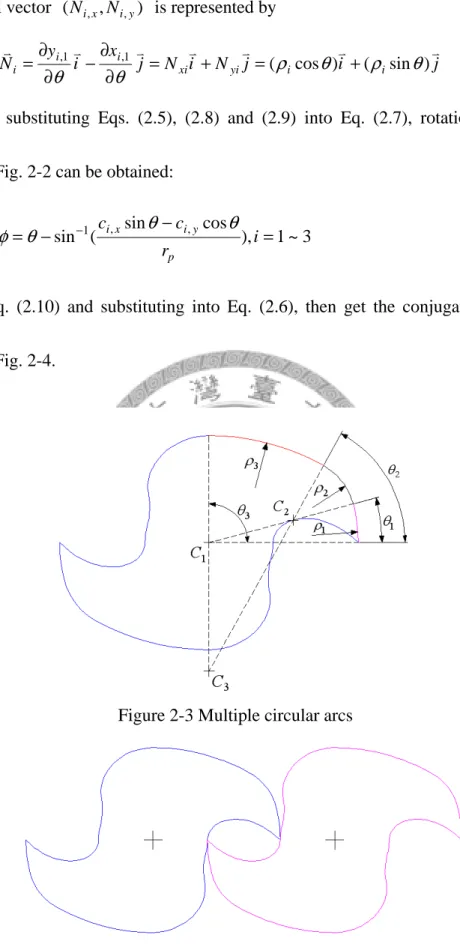
Figure 2-3 Multiple circular arcs ... 18

Figure 2-4 A pair of mating rotors ... 18

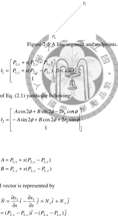
Figure 2-5 A line segment and endpoints ... 19

Figure 2-6 Line segment with the conjugate curve ... 20

Figure 2-7 Design parameters of epitrochoidal curve ... 21

viii

Figure 2-8 Generation of a epitrochoidal curve ... 21

Figure 2-9 Optimum design processes ... 25

Figure 3-1 Transverse tooth profiles for claw rotors ... 28

Figure 3-2 Contour of arc A and curve A’ ... 30

Figure 3-3 Contour of arc B and curve B’ ... 31

Figure 3-4 Contour of line G and curve G’ ... 32

Figure 3-5 Contour of arc F and curve F’ ... 33

Figure 3-6 Contour of epitrochoidal curves E and E’ ... 34

Figure 3-7 Contours of rotors and offsetting rotors ... 35

Figure 3-8 Relation between parameter and point ... 36

Figure 3-9 Instant contact point of rotors ... 36

Figure 3-10 Processes of the rotational angle calculation ... 36

Figure 3-11 Rotational angle of rotors

37 _°

... 37

Figure 3-12 Instant contact point presented in

S

₁ ... 37

Figure 3-13 Instant contact point presented in

S

_f ... 38

Figure 3-14 Pair of two meshing rotors ... 39

Figure 3-15 Amplified image of part of meshing ... 39

Figure 3-16 Relation between d and value of gap ... 40

Figure 3-17 Clearance between rotor and chamber ... 40

Figure 3-18 Effect of offset on clearance ... 41

Figure 4-1 Model of clearance between rotors and chamber ... 42

Figure 4-2 Coordinate system and notation used in analysis ... 43

Figure 4-3 Clearances between rotors ... 44

Figure 4-4 A simple leakage model ... 44

ix

Figure 4-5 Sketch map of axial leakage ... 47

Figure 4-6 Sketch map of radial leakage ... 47

Figure 4-7 Equipments of experiment ... 48

Figure 4-8 Steel claw rotors ... 48

Figure 4-9 Contour with offset ... 49

Figure 4-10 Real and theoretical flow rates of rotor pump with 0.06 offset ... 50

Figure 4-11 Real and theoretical flow rates of rotor pump with 0.08 offset ... 50

Figure 4-12 Definition of ideal flow rate ... 51

Figure 4-13 Rotors with undercutting ... 51

Figure 4-14

_∇

₁ of Set 1 ... 52

Figure 4-15

_∇

₂ of Set 1 ... 53

Figure 4-16 Rotors without undercutting ... 53

Figure 4-17

∇

₁ of Set 2. ... 53

Figure 4-18

_∇

₂ of Set 2.. ... 53

Figure 4-19 The effect of parameter

r on rate of leakage ... 54

_p Figure 4-20 Contour of driving rotor with different parameter

r

_p ... 54

Figure 4-21 Contour of driving rotor with different parameter D ... 55

Figure 4-22

_∇

₁ of Set 2. ... 55

Figure 4-23 The effect of parameter α on rate of leakage ... 56

Figure 4-24 Contour of driving rotor with different parameter α ... 56

Figure 4-25 The effect of parameter n on rate of leakage ... 57

Figure 4-26 Contour of rotor pair with different parameter n ... 57

Figure 4-27 Process and results of the optimum design of rotor with 5 claws ... 60

x

Figure 4-28 Process and results of the optimum design of rotor with 2 claws ... 61

Figure 4-29 Optimum design rotor with 5 claws ... 62

Figure 4-30 Optimum design rotor with 2 claws ... 62

Figure A-1 AutoCAD text window ... 70

Figure A-2 Loading the leakage program ... 72

Figure A-3 Leakage calculation commands (drawrotor) ... 73

Figure A-4 Design parameter inputting ... 73

Figure A-5 Contour and leakage flow rate of rotors ... 73

Figure B-1 Loading the undercutting identification program ... 77

Figure B-2 undercutting identification commands (drundercut) ... 77

Figure B-3 Design parameter inputting ... 77

Figure B-4 The response when undercutting occurs in rotor ... 77

Figure B-5 The response when rotor without undercutting ... 78

xi

List of Tables

Table 3-1 Calculation of d corresponding gap ... 39

Table 4-1 Parameters of steel claw rotor ... 48

Table 4-2 Relation between parameters and undercutting ... 52

Table 4-3 Relation between

r and

_p

D

_min ... 57

Table 4-4 Relation between n and pmin

r

... 58

Table 4-5 Variables for optimum design ... 59

Table 4-6 Value of object function for optimum design (n = 5) ... 60

Table 4-7 Value of object function for optimum design (n = 2) ... 61

Table 4-8 Variables for optimum design ... 61

1

Chapter 1 Introduction

This chapter introduces the basic knowledge of claw liquid pumps. The comparison and the development of claw liquid pumps are the main topics of this chapter.

1.1 Background and Motivation

The claw type rotors have been widely applied in many industries. They are used in liquid pumps, vacuum pumps, and compressors. The pumps with claw type rotors are positive displacement rotary machines comprised essentially of a pair of meshing rotors contained in a casing and other chambers. The volume vary with rotation of rotors, and it also produces the pressure difference to transfer fluids from one place to another. The classification of pumps is shown in Fig. 1-1, and the claw rotor pumps belong to rotary pumps.

2

Figure 1-1 The pump universe [1].

To avoid crash and excessive frictional force, the contact between rotors and chamber of claw rotor with zero-clearance is inappropriate. Effective clearance is necessary, and it’s called ‘offset’ in the thesis. However, the existence of pressure difference will cause leakage if the fluid through the clearance between rotors and chamber [2].

The performance of liquid pump depends on volumetric efficiency, but the leakage will reduces pump efficiency. Paths of leakage are between rotors and chamber, and the main paths are nearby the contact point. Profile of rotor affects not only volumetric flow rate but also leakage flow rate. Discussing the relationship between profile and performance of rotors is essential. Moreover, different shapes of the rotors depend on the design parameters, and the feasible design regions of the parameters are discussed for avoiding the undercutting of rotors.

3

This study presents mathematical models of rotors to predict the leakage and for determine the feasible design region for avoiding the undercutting. Finally, this study will indicate the optimum design of claw rotors, and the processes are also described in detail. The result can indicate a better design course of parameters for designer.

1.2 Classification of rotary pump

In this chapter, most of rotary pumps which are similar to gear pump which are introduced, and the principle, advantages and disadvantage of pumps would be described briefed. Because of the emphasis of this thesis is aimed at claw pump, many varied claw pumps will be discussed in chapter 1.3.

a. Gear pump

Gear pumps can be divided into external and internal gear types [3]. A typical external gear pump is shown in Fig. 1-2. However, the external gear pump uses two identical gears, one gear is driven by a motor and it in turn to drives the other gear.

The fluid carried between the teeth of two meshing gears. The advantages of external gear pumps are high speed, high pressure, no overhung bearing loads, relatively quiet operation and design accommodates wide variety of materials. The disadvantages are no solids allowed and fixed end clearances.

4

Figure 1-2 External gear pump [3].

Internal gear pumps have a internal gear and an external gear [3]. There are gerotor pump and crescent pump, as shown in Figs. 1-3 (a) and (b), respectively. It can be observed that teeth number of inner gear is less than outer gear, and the fluid travels through the pump between the teeth, and the crescent shape divides the fluid and acts as a seal between the suction and discharge ports. The advantages of internal gear pumps are excellent for high-viscosity liquids, constant and even discharge regardless of pressure conditions and easy to maintain. The disadvantages are usually requires moderate speeds, medium pressure limitations.

Figure 1-3 (a) Gerotor pump [3].

5

Figure 1-3 (b) Crescent pump [3].

b. Lobe pump

The lobe pumps are belonging to rotary, external gear pumps [3], as shown in Fig. 1-4. It's different between lobe pump and external bear pump. One gear drives the other in a gear pump, but in a lobe pump, both lobes are driven through gears outside the pump casing chamber. The advantages of lobe pump are no obvious contact between rotors, accept to pass medium solids and appropriate in long term dry run.

The disadvantages of lobe pump are requires timing gears and reduced life with thin liquids.

Figure 1-4 Lobe pump [3].

6

c. Screw pump

Screw pumps are belong to axial flow gear pump [3], as shown in Fig. 1-5. The inlet hydraulic fluid that surrounds the rotors is carried as the rotors rotate and the direction is along the axis, until the fluid is forced out the outlet. The fluid does not rotate with the screw pumps, but moves linearly. The advantages of screw pumps are wide range of flows, pressures and viscosities, low mechanical vibration, pulsation free flow and easy to maintain. The disadvantages of screw pumps are relatively high cost because of close tolerances and running clearances, performance characteristics sensitive to viscosity change, high pressure capability requires long pumping elements.

Figure 1-5 Screw pump [3].

1.3 Profile of claw rotors

The first claw type rotor is mentioned in US patent 5,046,934 [4]. The pump includes a rotor pair and at least one chamber. The rotor pair is shown in Fig. 1-6.

7

Hsieh [5] presents a simple mathematical model for this claw rotor. There are two identical rotors, and the components of rotor profile are shown in Fig. 1-7. First rotor comprises circular surface and epitrochoidal curves. Circular surfaces, 1 and 4 are

conjugate, and epitrochoidal curves 2, 3 and 5 are generated by cusps ^P1,^P2 and ^P3, respectively.

Figure 1-6 Twin shaft vacuum pump [4].

Figure 1-7 The components of rotor profile [5].

The other claw type rotor is a stepped-disc pump with two identical rotors proposed in US patent 4,543,048 [6], and this pump has widely applications, as shown in Fig. 1-8. It comprises circular and epitrochoidal surfaces, as shown in Fig. 1-9.

8

Circular surfaces 1 and 2 are conjugate with each others, and epitrochoidal curve 3 is generated by cusp

P

₁. In the studies of Fong et al. [7] and Feng et al. [8], the rotors discussed are similar stepped-disc rotors, but they have distinct teeth shape, as shown in Fig. 1-10.

Figure 1-8 Stepped-disc pump [6].

Figure 1-9 The components of stepped-disc rotor [6].

Figure 1-10 Rotors which are similar stepped-disc rotor [7, 8].

Next pump is published in US patent 2005/0095160 A1 [9]. This pump includes a body, first rotor and second rotor. First rotor comprises a circular surface and a

9

blade, and second rotor comprises a circular surface and an engaged recess. Each center of circular is center of rotor, and the summation of circular radius is the distance of centers. The blade of first rotor is formed with three mating surfaces, 311, 312 and 313, as shown in Fig. 1-11. The engaged recess of second rotor comprises three mating surfaces, 411, 412 and 413, and is conjugate with the blade of first rotor.

Observed from Fig. 1-11, epitrochoidal curve 311 is generated by cusp of surface 411 and circular surface, and curve 411 is generated by cusp of surfaces 311 and 313.

Contour of first rotor is symmetrical reflection curve, and the second rotor is, too. The processes of rotors’ rotating are shown as Fig. 1-12.

Figure 1-11 The components of rotors [9].

Figure 1-12 Processes of rotors’ rotating [9].

10

Finally, these kinds of claw rotors are similar, but tooth root and tooth crown composed of different curves. The rotor shown in Fig. 1-13 which mentioned in US patent 5,667,370 [10] comprises circular and epitrochoidal curves. The other curve is defined by archimedean curve. However, the contour of rotors published in US patent 5,697,772 [11] also comprises circular and epitrochoidal curves, as shown in Fig. 1-14.

But the other curves is defined by a tooth profile curve generated by the imaginary rack formed a sine curve, as shown in Fig. 1-15.

Figure 1-13 Contour of rotor formed archimedean curve [10].

Figure 1-14 Contour of rotor generated by the imaginary rack [11].

11

Figure 1-15 Imaginary rack formed a sine curve [11].

1.4 Paper review

There are several study proposed the mathematical model of rotor to measure the performance. Cao et al. [12] presented mathematical model of twin-screw rotor and evaluating the inter-lobe clearance. And discussed the characteristic with geometry parameter, the given stock δ . Fong et al. [7] presented a mathematical procedure to calculate the inter-lobe clearance between two mating screw rotors, and uses iso-clearance contour diagram (ICCD) to determine the size and shape of overlapped cavity and the complete inter-rotor clearance. Fleming et al. [13] developed a computer program to analysis the leakages of a refrigeration helical screw compressor and identified six separate types of leakage path. And a mathematical model of the complete compressor thermo-fluid process is constructed. Su et al. [14] presented optimization problems where the object function is the contact-line length and the blowhole area is the constraint. It provides a useful suggestion for rotor-profile optimization of the screw compressor. Wang et al. [15] proposed a design procedure

12

for determining the feasible region of design parameters considering the geometry constraints, zero carryover and non-undercutting.

13

Chapter 2 Related theories of claw liquid pumps

This chapter introduces the related theories for claw liquid pumps. The brief description of conjugate surface theory, coordinate transformation matrix, mathematical model of geometric model, and design processes are shown as following

2.1 Conjugate surface theory

Conjugate motion is geometrically constrain through contacts between boundary surfaces. These boundary surfaces have to keep contact with each other during the motion, and they are called conjugate surfaces. The conjugate motion obeys the conjugate theory, and involves at least two bodies.

The theory of Conjugate Surfaces [16], discusses the law of inter-relationship between two entities. One is the geometrical configurations, another is the conjugate motion. The configurations must have a base and a mate surface, such as femur and tibia in the knee joint, respectively. However, conjugate motion is defined as such relative motion between the two meshing solids, which have the continuous contact between boundaries. The theory consists of 4 parts. They are Solid body motion representation: ration of vector, Kinematical representation of geometry: engineering differential geometry, Kinematics of conjugate motion, and Geometry of conjugate

14

configurations. According these theories, the base and mate surfaces can be expressed together with a relevant conjugate motion. Meanwhile, the theory also provides an efficient algorithm for computing the known conjugate surfaces.

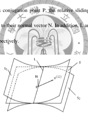
Two basic feature of instantaneous conjugate motion[17]: At any instant of a conjugate motion, there exists at least one instantaneous conjugation point (ICP) between a pair of conjugate surface. As shown in Fig. 2-1, owing to keeping continuous conjugation between the two conjugate surfaces

S

₁ and

S

₂ at the

relevant instantaneous conjugation point P, the relative sliding velocity

V

⁽¹²⁾ at P must be perpendicular to their normal vector N. In addition, L and T is the sets of ICP and tangent plane, respectively.

Figure 2-1 Conjugate surface.

2.2 Coordinate transformation matrix

15

In the two-dimensional space, transformation of two Cartesian coordinate systems may use the matrix of rotations and translations, and their relation can be calculated described with geometric graph.

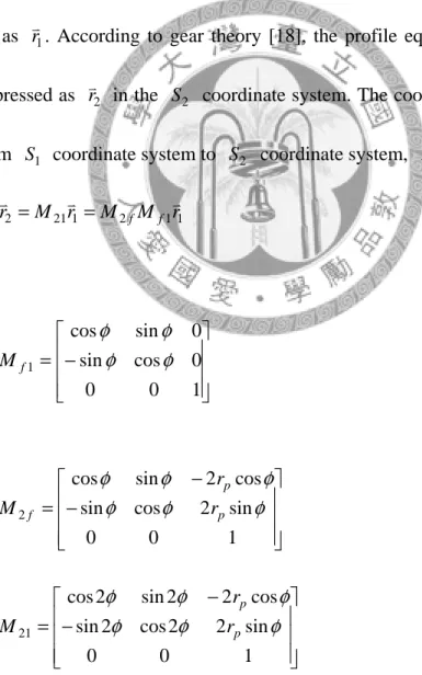
Fig. 2-2 represents the coordinate systems of two mating rotors. Movable coordinate systems

S

₁

( X

₁

, Y

₁

, Z

₁

)

and

S

₂

( X

₂

, Y

₂

, Z

₂

)

are rigidly connected to the generating surface and generated surface, and

S

_f(

X

_f,

Y

_f,

Z

_f ) is a fixed coordinate system. The profile equation of driving rotor in the

S

₁ coordinate system may be expressed as

r

₁. According to gear theory [18], the profile equation of driven rotor can be expressed as

r

₂ in the

S

₂ coordinate system. The coordinate transformation matrix from

S

₁ coordinate system to

S

₂ coordinate system,

M

₂₁, as follows:

1 1 2 1 21

2

M r M M r

r

 =  = _{f f}  (2.1)

where

 







 







−

=

1 0 0

0 cos sin

0 sin cos

1 φ φ

φ φ

M

f (2.2)

 







 







−

−

=

1 0

0

sin 2 cos sin

cos 2 sin

cos

2 φ φ φ

φ φ

φ

p p

f

r

r

M

(2.3)w

 







 







−

−

=

1 0

0

sin 2 2 cos 2

sin

cos 2 2 sin 2

cos

21 φ φ φ

φ φ

φ

p p

r r

M

(2.4)

16

where

φ

is the angle of rotation of the driving rotor

Figure 2-2 Coordinate systems for generating mating rotors [19].

2.3 Mathematical model of model geometry

The transverse tooth profiles of claw rotors can be described in mathematical model by the theory of conjugate surfaces and the coordinate transformation matrix.

The profile of driving rotor is composed of arcs, line segments and epitrochoid curves.

The position vectors of these curves and the corresponding conjugate curves will be proposed in this chapter.

2.3.1 Mathematical model of circular arcs

The position vector of the multiple circular arcs,

r

_i,1=(

x

_i,1,

y

_i,1), as shown in Fig. 2-3 are represented in coordinate system

S

₁as follows:

17

3

~ 1 , ,

1 sin cos

1 ,

, 1

,

≤ < =

 







 





 + +

= c

₋

i

c

r

_{iy i i i}

i x i

i ρ θ θ θ θ

θ



ρ (2.5)

where 0

θ

₀ = ^{, )}

C

i =⁽

c

i,x^,

c

i,y are the center of three circular arcs, and the definition of

ρ

_i^,

θ

i as shown in Fig. 2-3.

substituting Eq. (2.5) into Eq. (2.1):

 







 







+ +

−

−

− +

+

−

=

1

sin 2 2 cos 2

sin )

2 sin(

cos 2 2 sin 2

cos )

2 cos(

, ,

, ,

2

,

ρ θ φ φ φ φ

φ φ

φ φ

θ ρ

p y

i x

i i

p y

i x

i i

i

c c r

r c

c

r

(2.6)

where

r

_i,2 is the position vector of the curves conjugated with

r , presented in

_i,1 coordinate system

S

₂.

The equation of meshing [18] between mating rotors are obtained as following:

0 )

, (

, 1 , ,

1

,

− =

− −

=

y i

i x

i i

N y Y N

x

f

θ φ

X

(2.7)

where (X, Y) is the Cartesian coordinate of instantaneous center P presented in coordinate system

S

₁. The (

x

_i,1,

y

_i,1) and the (

N

_i,x,

N

_i,y) are the Cartesian

coordinate and the normal vector of instant contact point presented in coordinate system

S

₁, respectively. The Cartesian coordinate of (X, Y) as following:

φ φ

sin

cos

p p

r Y

r X

=

=

(2.8)

18

the normal vector (

N

_i,x,

N

_i,y) is represented by

j i

j N i N x j

y i

N 

_i ⁱ



ⁱ



_xi



_yi



_i



_i



) sin ( ) cos

1

(

, 1

, ρ θ ρ θ

θ

θ

∂ ^{= + = +}

− ∂

∂

= ∂

(2.9)

thereafter, substituting Eqs. (2.5), (2.8) and (2.9) into Eq. (2.7), rotation angle as shown in Fig. 2-2 can be obtained:

3

~ 1 cos ),

( sin

sin ^{1 ,} − ^, =

−

= ⁻

i

r c c

p y i x

i

θ θ

θ

φ

^(2.10)

solving Eq. (2.10) and substituting into Eq. (2.6), then get the conjugate curve, as shown in Fig. 2-4.

Figure 2-3 Multiple circular arcs

Figure 2-4 A pair of mating rotors.

19

2.3.2 Mathematical model of a line segment

The equation of the line segment, where the endpoints are

P

₁ =(

P

_1,x,

P

_1,y)and )

, ( _{2, 2,}

2

P

x

P

y

P

= as shown in Fig. 2-5 is represented in coordinate system

S

₁as

follows:

Figure 2-5 A line segment and endpoints.

1 0

, 1

) (

) (

1 , 2 ,

1

1 , 2 ,

1

1

< <

 







 







− +

− +

= P s P P s

P P s P

r

_{y y y}

x x



x (2.11)

operation of Eq. (2.1) yields the following:

 







 







+ +

−

− +

=

1

sin 2 2 cos 2

sin

cos 2 2 sin 2

cos

2

φ φ φ

φ φ

φ

p p

r B

A

r B

A

r

(2.12)

where

) (

) (

, 1 , 2 ,

1

, 1 , 2 ,

1

y y y

x x x

P P s P B

P P s P A

− +

=

− +

=

(2.13)

the normal vector is represented by

j P P i P P

j N i N s j i x s N y

x x y

y

y x











 

) (

)

( _{2, 1, 2, 1,}

1 1

−

−

−

=

+

∂ =

−∂

∂

= ∂

(2.14)

20

substituting Eqs. (2.8), (2.11) and (2.14) into equation of meshing Eq. (2.7), rotation angle can be described as following:

1

D

sin⁻ +

−

=

α

φ

^(2.15)

where

2 , 1 , 2 2 , 1 , 2

, 1 , 2 ,

1 , 2

2 , 1 , 2 2 , 1 , 2

, 1 , 2 1

) (

) (

) (

) (

) ) (

) (

( sin

y y x

x p

y y x

x

y y x

x

x x

P P P

P r

P P B P P D A

P P P

P

P P

− +

−

− +

= −

− +

−

= ⁻ −

α

(2.16)

solving Eq. (2.15) and substituting into Eq. (2.12), then get the conjugate curve, as shown in Fig. 2-6.

Figure 2-6 Line segment with the conjugate curve.

2.3.3 Mathematical model of a epitrochoidal curve

An epitrochoidal curve is a roulette traced by a point attached to a rolling circle with radius

r

₂ around the outside of a fixed circle of radius

r

₁, where the point has a distance L from the center of the rolling circle, as shown in Fig. 2-7. The process of generating epitrochoidal curve is shown in Fig. 2-8.

21

Figure 2-7 Design parameters of epitrochoidal curve.

Figure 2-8 Generation of a epitrochoidal curve.

Equation of epitrochoidal curve presented in coordinate system

S

₁ as follows:

β θ θ θ

θ θ

≤

≤

 







 







+ +

−

− +

= , 0

1

2 sin sin

) (

2 cos cos

) (

2 1

2 1

L r

r

L r

r

r

(2.17)

where

2 ) ( cos ^{1 1 2}

L r r

+

= ⁻

β

^(2.18)

22

2.4 Conditions of non-undercutting

From the theory of gearing [18], the general conditions of non-undercutting have been determined. Because of singular points on driven rotor profile will cause undercut in the generation process, it may be represented by equation

) 0

12 ( ) 1 ( ) 2

( =

V

+

V

=

V

_{r r} (2.19)

if

V

_r⁽¹⁾ is function of

θ

, Eq. (2.19) yields

) 12 ( 1

1

V

dt r d

−

∂ =

∂ θ

θ

^(2.20)

and differentiated equation of meshing Eq. (2.7) 0

)]

, (

[

^f θ φ

=

dt

d

(2.21)

Eq. (2.21) yields

dt d f dt

d

f φ

φ θ

θ

∂

−∂

∂ =

∂ (2.22)

Eqs. (2.20) and (2.22) represent a system of three linear equations in one unknown:

^d

θ /

dt

. This system has a certain solution for the unknowns if the matrix

 

 





 

 





∂

− ∂

∂

∂

∂ −

∂

=

dt d f f

r V

A φ

φ θ

θ

) 12 ( 1 1

(2.23)

has the rank r=1. In addition

r 

₁

= ( x

₁

, y

₁

)

is the position vector of driving rotor and represented in coordinate system

S

₁. This yields

23

0 0

) 12 (

, 1 1

2

) 12 (

, 1 1

1

=















−

∂ −

∂

=

∇

=















−

∂ −

∂

=

∇

dt f d f

y v

dt f d f

x v

y x

θ φ θ φ

φ θ

φ θ

(2.24)

where

) (

] ) [(

) ,

( ₁⁽¹²_, ⁾ ₁⁽_,^{12) (1) (2)} ₁ ⁽²⁾

) 12

(

v v

=

ω

−

ω

×

r

−

E

×

ω

V

_{x y} (2.25)

and

E

is vector

O

₁

O

₂ in system

S

₁, where

O

₁,

O

₂ are centers of driving rotor and driven rotor, respectively.

2.5 Optimum Design Theorem

In general, an optimization problem comprises three items: design variables, objective function, and constraints. The object of optimum design is to improve the structural characteristics or reduce the cost of the product. The design variables are usually the sizes of members in the structure, such as thickness of a plate; the configuration and geometry layout of the problem, such as location parameters of a component; the physical properties of a material, such as young’s modulus of a material. The design variables should be selected to represent the structural characteristics. Too many design variables will affect the efficiency for searching optimum solutions. The objective function is a function of design variables. The

24

function is usually the structural weight or distortion of the structure. The objective function is decided by the user for different considerations. Generally, design constraints in engineering can be sorted into size constraints and behavior constraints.

Size constraints mean the restriction range of the design variables, and behavior constraints represent requirements of the structural performance or response, such as the displacement and the stress in the structure.

The structural optimum design problem can be represented as Eq. (2.26), where

x are design variables, F  is the objective function,

( x)

g

_j( x) is the constraint, and

n is the number of constraints.

_c

Find

x

Such that

F 

( x)^→min. (2.26)

Subject to

g

_j( x) _≤0, i=1,2…,

n

_c

The initial process for optimization problem is to establish the system model, define the design variables, objective function, and constraints, and then get the initial value of the objective function from initial values of design variables. Iterative search method is the next step to get new design variables, and a new objective function value by these new design variables will be obtained. If the new objective function value does not converge, the search iteration will go on until finding convergent

25

solutions, which are also the optimum solutions. Fig. 2-9 shows the process of solving optimization problems.

Collect data to describe the

system

Identify design variables, objective function,

constraints

Analyze the system to find objective function and

constraints

Check convergent and feasible ?

Optimum design Redesign

Yes No

Figure 2-9 Optimum design processes.

In the optimum design process described above, the most common ways to do iterative search for optimum solution are non-linear programming or genetic algorithm. The non-linear programming method is a traditional search method for optimum solution. The non-linear programming method needs one set of initial value, decides the search direction by gradient theorem, and processes the next search by the known information. This method can converge to the optimum solution in a region accurately and quickly.

26

2.6 Design process

The steps of design process are shown as following:

Step 1: Set up the plane coordinate systems of rotors.

Step 2: Give the equation of the transverse tooth profiles for driving rotor.

Step 3: Solve equation of meshing.

Step 4: Solve mathematical model of the transverse tooth profiles for driven rotor by the operation of the coordinate transformation.

Step 5: Decide parameters and check whether parameters conform to the conditions of undercutting or not.

27

Chapter 3 Meshing conditions of claw rotors

In this chapter, the claw rotor published in US patent 7,565,741 [20] would be introduced. It is regard as an example to illustrate the processes of calculating clearance by mathematical model.

3.1 Design of claw rotors

The new claw rotor pair presented in this paper consists of a driving rotor and a driven rotor. For the driving rotor, the contour of each claw is composed of 5 curve entities: arc A, arc B, arc F, line G and epitrochoidal curve E, as shown in Fig. 3-1.

Entity data of these 5 curve entities are determined by five significant parameters, namely radius of rotor R, radius of pitch circle

r , depth of claw D, angle

_p α of arc

A, and number of claws n. It is also noted that distance between two rotor centers is2

r

_p. By referencing Fig. 3-1, detail procedure to define these 5 entities can be

expressed as:

(a). Curve E is an epitrochoidal curve obtained by rolling the driven pitch circle onto the outside of the driving pitch circle.

(b). Arc A is define by the center point

C

₁, two end point

P ,

₀

P

₁ with arc angle

α

^.

28

(c). Arc B is defined by its center

C

_B, located in line

C

₁

P

₁ and the half distance D/2 is distance between the highest point of arc B and line

C

₁

C

₂. With the above relation, the radius of the arc B can be obtained as,

α ρ α

α ρ

ρ 1 sin

sin 2 / sin 2

)

( −

= −

→

=

−

+ D D R

R _{B B}

B (3.1)

(d). Arc F is define by the center point

C

₁, radius ρ . The radius of arc F is _F defined as:

R r

_p

F

= 2 −

ρ

(3.2)

(e). Line G is the outer common tangent of arcs B and F. The tangent points are

P

2 and

P .

₃

New type claw rotors defined by this method have two distinct rotors, and the driving rotor and the driven rotor are totally different. The curves mentioned above are curve entities of one claw only, and the profile of the whole rotor can be obtained by n copies of one claw curve entities.

Figure 3-1 Transverse tooth profiles for claw rotors [20].

29

3.2 Mathematical model of claw rotors

The equation of transverse sections of driving rotor

r

₁

( x

₁

, y

₁

)

and driven rotor

)

, (

_{2 2}

2

x y

r

are derived in the coordinate systems

S

₁(

x

_1,

y

₁,

z

₁) and

S

₂(

x

_2,

y

₂,

z

₂), respectively.

a. Profile of circular arc A and the conjugate curve

As shown in Fig. 3-1,

C

_A

= C

₁

= ( 0 , 0 )

, ρ_A

= R

and θ_A

=

α , according the theory in Chapter 2.3.1, the mathematical model of the circular arc A and the conjugate curve can be described in the coordinate system

S

₁ as follows:

 

 ≤ <

=

=

θ α

θ θ

, 0 sin cos

1 1

R y

R

x

(3.3)

 



+

−

=

−

−

=

φ φ

θ

φ φ

θ

sin 2 ) 2 sin(

cos 2 ) 2 cos(

2 2

p p

r R

y

r R

x

(3.4)

the rotation angle

θ

φ

= (3.5)

Substituting Eq. (3.5) into Eq. (3.4) then gets the conjugate curve. Contours of arc A and the conjugate curve A’ are shown in Fig. 3-2.

30

Figure 3-2 Contour of arc A and curve A’.

b. Profile of circular arc B and the conjugate curve

As shown in Fig. 3-1, C_B =(

c

_B,x,

c

_B,y) and sin ( ) 2

1 B

B F B

R ρ ρ ρ θ π

− + −

= ⁻

according the theory in Chapter 2.3.1, the mathematical model of the circular arc B and the conjugate curve can be described in the coordinate system

S

₁ as follows:

)]

( 2 sin [

sin ,

cos

₁

, 1

, 1

B F B B

y B

B x B

c R y

c x

ρ ρ ρ α π

θ θ α ρ

θ ρ

− + −

+

<

 ≤

 

+

= +

=

₋

(3.6)

 



+ +

−

−

=

− +

+

−

=

φ φ

φ φ

θ ρ

φ φ

φ φ

θ ρ

sin 2 2 cos 2

sin )

2 sin(

cos 2 2 sin 2

cos )

2 cos(

, ,

2

, ,

2

p y

B x

B B

p y

B x

B B

r c

c y

r c

c x

(3.7) where

c

B,x =⁽

R

−

ρ

B^)cos

α

,

c

B,y =⁽

R

−

ρ

B^)sin

α

the rotation angle

cos ) ( sin

sin

^{1 , ,}

p y B x

B

r c

c θ θ

θ

φ = −

⁻

⁻

(3.8)

substituting Eq. (3.8) into Eq. (3.7) then gets the conjugate curve, the contour of arc B and the conjugate curve B’ are shown in Fig. 3-3.

31

Figure 3-3 Contour of arc B and curve B’.

c. Profile of line G and the conjugate curve

As shown in Fig. 3-1

P

₂ =(

P

_2,x,

P

_2,y)and )

P

₃ =(

P

_3,x,

P

_3,y are endpoints of line

G. According the theory in Chapter 2.3.2, the mathematical model of the line G and the conjugate curve can be described in the coordinate system

S

₁ as follows:

 

 = + − ≤ ≤

− +

= , 0 1

) (

) (

, 2 , 3 ,

2 1

, 2 , 3 ,

2

1

s

P P s P y

P P s P x

y y y

x x

x (3.9)

















− + −

+

− + −

+

=



 





















− + −

+ +

−

− + −

+ +

−

=



 





−

−

−

−

)]

( 2 sin sin[

)]

( 2 sin cos[

)]

( 2 sin sin[

sin ) (

)]

( 2 sin cos[

cos ) (

1 1

, 3 , 3

1 1

, 2 , 2

B F B F

B F B F

y x

B F B B

B

B F B B

B

y x

R R P

P

R R R R P

P

ρ ρ ρ α π

ρ

ρρ ρ α π

ρ

ρρ ρ α π

ρ α ρ

ρρ ρ α π

ρ α ρ

(3.10)

) (

) (

sin 2 2 cos 2

sin

cos 2 2 sin 2

cos

, 2 , 3 ,

2

, 2 , 3 ,

2 2

2

y y y

x x x

p p

P P s P v

P P s P u

r v

u y

r v

u x

− +

=

− +

=

 



+ +

−

=

− +

=

φ φ

φ

φ φ

φ

(3.11)

the rotation angle is

1

w sin

⁻

+

−

= ψ

φ

(3.12)

where,

32

2 , 2 , 3 2 , 2 , 3

, 2 , 3 ,

2 , 3

2 , 2 , 3 2 , 2 , 3

, 2 , 3 1

) (

) (

) (

) (

) ) (

) (

( sin

y y x

x p

y y x

x

y y x

x

x x

P P P

P r

P P v P P w u

P P P

P

P P

− +

−

− +

= −

− +

−

=

⁻

− ψ

(3.13)

substituting Eq. (3.12) into Eq. (3.11) then gets the conjugate curve, the contour of line G and the conjugate curve G’ are shown in Fig. 3-4.

Figure 3-4 Contour of line G and curve G’.

d. Profile of circular arc F and the conjugate curve

As shown in Fig. 3-1,

C

_F

= C

₁and _{A B}

n π θ θ θ

= 2 − −

F , according the theory in Chapter 2.3.1, the mathematical model of the circular arc F and the conjugate curve can be described in the coordinate system

S

₁ as follows:

n R

y x

B F B F

F

θ π ρ

ρ π ρ

α

θ ρ

θ ρ

)] 2 (

2 sin [

sin cos

1 1

1

<

− ≤ + −

+





=

=

−

(3.14)

 



+

−

=

−

−

=

φ φ

θ ρ

φ φ

θ ρ

sin 2 ) 2 sin(

cos 2 ) 2 cos(

2 2

p F

p F

r y

r

x

(3.15)

the rotation angle

θ

φ

= (3.16)

33

substituting Eq. (3.16) into Eq. (3.15) then gets the conjugate curve, the contour of arc F and the conjugate curve F’ are shown in Fig. 3-5.

Figure 3-5 Contour of arc F and curve F’.

e. Profile of epitrochoidal curves E and E’

As shown in Fig. 3-1, the rolling circle and base circle of epitrochoidal curve E are pitch circles of driven rotor and driving rotor, respectively. Substituting

r

p

r

=

= 2

r1 into Eqs. (2.17) and (2.18), the mathematical model of the epitrochoidal curve E can be described in the coordinate system

S

₁ as follows:

) ( cos

0 2 , sin sin

2

2 cos cos

2

1 1

1

R r

R r

y

R r

x

p p p

= −



 ≤ ≤

+

−

=

−

=

β

β θ θ

θ

θ θ

(3.17)

The rolling circle and base circle of epitrochoidal curve E’ are pitch circles of driving rotor and driven rotor, respectively. The mathematical model of the epitrochoidal curve E’ can be described in the coordinate system

S

₂ as follows:

β θ θ

θ

θ

θ ≤ ≤

 



−

=

+

−

= , 0

2 sin sin

2

2 cos cos

2

2 2

R r

y

R r

x

p

p (3.18)

34

However, epitrochoidal curves E and E’ are not conjugate with each other, and they are a roulette trace by

P and

₅

P , respectively. The contour of epitrochoidal

₀ curves E and E’ are shown in Fig. 3-6.

Figure 3-6 Contour of epitrochoidal curves E and E’.

3.3 Clearance calculation

To avoid crash and excessive frictional force, the contact between rotors and chamber of claw rotor cannot be without clearance. Effective clearance is necessary, and it’s called ‘offset’ in this thesis. However, the existence of pressure difference will cause leakage if the fluid through the clearance between rotors and chamber.

Effect of clearance cannot be neglected, thus calculating clearance between rotors and chamber is necessary. Offsetting creates a new contour, that every point on new contour has the same distance with point on original contour, as shown in Fig. 3-7.

35

Figure 3-7 Contours of rotors and offsetting rotors.

This study presents the course to calculate clearance between rotors and chamber.

First, obtain instant contact point in the whole conjugate motion. Second, calculate the clearance between rotors in the proximity of instant contact point. Finally, consider the affect of offset to clearance.

3.3.1 Instant contact point of rotors

The equations of driving rotor transverse profile are functions of θ or functions of s. Each θ has the corresponding rotation angle

φ

. The geometric meaning of

φ

will describe in detail.

According to mathematical model of driving rotor transverse profile, parameter θ has the corresponding point

P

1 at driving rotor, as shown in Fig. 3-8. Rotate

driving rotor clockwise and rotate driven rotor counterclockwise through angle

φ

^. Point

P

₁

'

is the instant contact point of rotors, as shown in Fig. 3-9, where

P

₁

'

is the point

P

₁ attached to driving rotor.

36

Figure 3-8 Relation between parameter and point.

Figure 3-9 Instant contact point of rotors.

Figure 3-10 Processes of the rotational angle calculation.

However, in the whole conjugate motion, rotation angle is a variable which easy to control and continuous. By numerical methods and interpolation, corresponding geometric variables θ and s could be obtained when

φ

is known. The instant

37

contact points in the whole conjugate motion are also determined. The steps of obtaining the coordinate of instant contact point as follow:

Step 1: The rotational angle

φ

is known, as shown in Fig. 3-11.

Step 2: Solve the parameters

θ

^or

^s

by numerical methods, and substituting parameters

θ

^or

^s

^into

r

1 to obtain instant point

P presented in coordinate

_c system

S

₁, as shown in Fig. 3-12.

Step 3: By transformation matrix, calculate coordinate of instant contact point

P

_c presented in the fixed coordinate system

S , as shown in Fig. 3-13.

_f

Figure 3-11 Rotational angle of rotors

37 _°

.

Figure 3-12 Instant contact point presented in

S

₁.