長方形彈性層黏著於剛性板的壓縮分析

行政院國家科學委員會專題研究計畫 成果報告

長方形彈性層黏著於剛性板的壓縮分析

計畫類別： 個別型計畫

計畫編號： NSC92-2211-E-011-033-

執行期間： 92 年 08 月 01 日至 93 年 07 月 31 日 執行單位： 國立臺灣科技大學營建工程系

計畫主持人： 蔡相全

計畫參與人員： 黃俊智,林育民

報告類型： 精簡報告

處理方式： 本計畫涉及專利或其他智慧財產權，2 年後可公開查詢

中 華 民 國 93 年 9 月 17 日

行政院國家科學委員會補助專題研究計畫成果報告 長方形彈性層黏著於剛性板的壓縮分析

計畫類別：√ 個別型計畫 □ 整合型計畫 計畫編號：NSC 92－2211－E－011－033

執行期間：92 年 8 月 1 日至 93 年 7 月 31 日

計畫主持人：蔡相全

計畫參與人員：黃俊智，林育民

成果報告類型(依經費核定清單規定繳交)：√ 精簡報告 □完整報告

本成果報告包括以下應繳交之附件：

□赴國外出差或研習心得報告一份

□赴大陸地區出差或研習心得報告一份

□出席國際學術會議心得報告及發表之論文各一份

□國際合作研究計畫國外研究報告書一份

處理方式：除產學合作研究計畫、提升產業技術及人才培育研究計畫、列 管計畫及下列情形者外，得立即公開查詢

□涉及專利或其他智慧財產權，□一年√ 二年後可公開查詢

執行單位：國立台灣科技大學營建工程系

中 華 民 國 93 年 7 月 31 日

摘要

橡膠層墊是由多層橡膠片黏著於薄鋼片之間所構成，由於在水平方向具有低勁度，

橡膠層墊用於橋樑工程以容許因溫度變化所產生的伸縮，也被用於基底隔震以減少建築 物因地震造成的振動。橡膠層墊須具有垂直向的剛性以承受上部結構的載重，而垂向的 剛性則來自於橡膠片的側向變位受制於所黏著的鋼片，如果橡膠片的黏著應力超過其強 度，橡膠片和鋼片的黏界面將開裂，導致橡膠承墊不穩定，而無法支承上部結構，因此 受鋼片束制之橡膠片的壓縮勁度和黏著應力在橡膠層墊的設計中極為重要。本研究計劃 的目的乃是去探討長方形橡膠層墊受到軸向壓力的壓縮勁度與所產生的黏著應力。研究 所用的分析模型是一長方形彈性層，其上下面分別黏著於一剛性板，根據兩個變形的基 本假設，利用彈性力學理論，求解出受剛性板束制之長方形彈性層的壓縮勁度公式與黏 著面的應力公式。所用的第一個變形假設為﹕平行於剛性板的平面斷面，在變形後仍然 保持一平面。第二個變形假設為﹕垂直於剛性板的直線，在變形後成為一拋物線。所推 導出理論公式適用範圍將不受柏松比與形狀係數的限制。本計劃亦將利用有限元素分析 法來証明所推導出理論公式的精確性。

關鍵詞﹕橡膠層墊，壓縮勁度，黏著應力。

Abstract

Laminated rubber bearings consist of thin sheets of rubber layers bonded to interleaving steel shims. Because of their low stiffness in horizontal direction, laminated rubber bearings are utilized in bridge engineering to allow temperature deformation and in base isolation to reduce building vibration induced by earthquakes. Laminated rubber bearings must possess sufficient rigidity to sustain the gravity loading of superstructures. The vertical rigidity is supplied from the restricted lateral expansion of rubber layers bonded with steel shims. If the bonding stress of rubber layers is larger than its strength, the bonding interface between rubber layers and steel shims will crack, which makes the laminated rubber bearing becomes unstable and cannot sustain the superstructure. Therefore, the compression stiffness and the bonding stress of rubber layers bonded by steel shims are very important for the design of laminated rubber bearings. The purpose of this research project is to study the stiffness and the bonding stresses developed under axial compression in rectangular laminated rubber bearings. The theoretical model is a rectangular elastic layer bonded between two rigid plates.

The compression stiffness of the bonded rectangular elastic layer and the bonding stress at the interface between the elastic layer and the rigid plate will be solved by the theory of elasticity based on the two kinematics assumptions. The first assumption is that plane sections parallel to rigid plates remain plane after deformation. The second assumption is that vertical lines normal to rigid plates become parabolic after deformation. The derived compression stiffness and bonding stress will applicable to any value of Poisson’s ratio and shape factor. This project will apply the finite element method to verify the accuracy of the derived formulae.

Keyword: Laminated rubber bearing, Compression stiffness, Bonding stress.

1. Introduction

When an elastic layer is bonded between two rigid plates, the rigid plates can restrict the lateral expansion of the elastic layer and result in the bonded elastic layer having higher compression stiffness than the elastic layer without bonding. The effect becomes more dramatic when Poisson’s ratio of the elastic layer is near 0.5. This characteristic has been adopted in the design of laminated elastomeric bearings that consist of many elastomeric layers bonded to interleaving steel plates. Laminated elastomeric bearings, employed in many fields such as seismic isolation, can provide high vertical rigidity to sustain gravity loading, while still providing the same horizontal flexibility as elastomer.

To analyze the stiffness of bonded layers, two kinematics assumptions are usually adopted: (i) planes parallel to the rigid bonding plates before deformation remain planar after loading; (ii) lines normal to the rigid bonding plates before deformation become parabolic after loading. Gent and Lindley (1959) derived the compression stiffness of an incompressible elastic layer for infinite-strip shape and circular shape. Subsequently, Gent and Meinecke (1970) extended this method to analyze the compression stiffness and tilting stiffness of incompressible elastic layers for square and other shapes.

Although rubber can be treated as incompressible in some analyses, the assumption of incompressibility tends to overestimate the compression stiffness and tilting stiffness of the bonded rubber layer when the layer's shape factor (defined as the ratio of the one bonded area to the force-free area) is high. Kelly (1997) developed a ‘pressure solution’ approach to derive the compression stiffness and the tilting stiffness considering the effect of bulk compressibility. The solutions are available for the layers of infinite-strip shape (Chalhoub and Kelly, 1991), circular shape (Chalhoub and Kelly, 1990) and square shape (Kelly, 1997).

Lindley (1979a) applied an energy method to derive the compression stiffness of the infinite-strip and circular shapes as well as the tilting stiffness of the infinite-strip shape (Lindley, 1979b) for the material of any Poisson's ratio. Koh and Kelly (1989) utilized a

‘variable transform’ approach to derive the compression stiffness of the square shape for compressible material. Koh and Lim (2001) extended this approach to solve the compression stiffness of the rectangular shape.

The stiffness of bonded layers is related to the vertical stress, which can be derived from the mean pressure. Tsai and Lee (1998 and 1999) developed a pressure approach to derive the compression stiffness and tilting stiffness of bonded elastic layers in infinite-strip, circular and square shapes. Recently, Tsai (2003) presented an approach to analyze the tilting stiffness of the circular shape by solving displacement directly. These solutions are accurate for the material of any Poisson's ratio.

To reduce the weight and the cost of laminated elastomeric bearings, the steel plates can be replaced by fiber reinforcement. In contrast to the steel reinforcement that is assumed to be rigid, the fiber reinforcement is flexible in extension. The compression stiffness and tilting

stiffness of fiber-reinforced bearings in infinite-strip, circular and rectangular shapes are derived by assuming the elastomeric layer is incompressible and the reinforcement is flexible (Kelly, 1999; Tsai and Kelly, 2001, 2002a, 2002b). Recently, bulk compressibility is also included in the stiffness analysis of fiber-reinforced bearings of the infinite-strip shape (Kelly, 2002; Kelly and Takhirov, 2002).

In this paper, the pressure approach by Tsai and Lee (1998) is extended to solve the compression stiffness of the rectangular layers bonded between rigid plates. Being different from the solution of Koh and Lim (2001) that is a double-series closed form, the present solution is a single-series closed form and has faster convergence. The displacements of the elastic layer and the bonding shear stresses on the interface of the elastic layer and the rigid plate are also derived. To verify the exactness of the theoretical solutions, finite element analyses are carried out, where the eight-node solid elements with incompatible bending modes is applied to model the elastic layer.

2. Solution of pressure

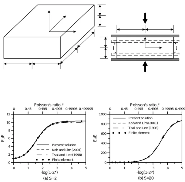
A rectangular layer of linearly elastic, homogeneous and isotropic material bonded between two rigid plates is shown in Fig. 1 where a Cartesian coordinate system (x, y, z) is located at the center of the layer. The elastic layer has a thickness of t, a width of 2a along the x-axis, and a length of 2b along the y-axis. Under a compression force in the z direction, the displacements of the elastic layer, u, v and w along the x, y and z directions respectively, can be assumed to have the form

4 ) 1 )(

, ( ) , ,

( ₂

2

t y z x u z y x

u = − (1)

4 ) 1 )(

, ( ) , ,

( ₂

2

t y z x v z y x

v = − (2)

) ( ) , ,

(x y z w z

w = (3)

where Eqs. (1) and (2) represent the assumption of quadratic deformation on vertical lines;

Eq. (3) represents the assumption that horizontal planes remain plane.

For isotropic elastic material, the mean pressure p has the following relation with the displacements

) (

) , ,

(x y z u_,x v_,y w_,z

p =−κ + + (4)

in which κ is the bulk modulus and the commas imply differentiation with respect to the indicated coordinate. The effective pressure p is the average pressure through the thickness, defined as

∫

= ^/2

2

/ ( , , )

) 1 ,

( ^t

t p x y z dz y t

x

p (5)

which becomes, when using the displacement assumptions in Eqs. (1) to (3),

c y

x v

p u ε

κ ⁼⁻3^{( + )+} 2

,

, (6)

where ε is the effective compression strain defined as _c )]

2 t ( w ) 2 t ( w t[ 1

c =− − −

ε (7)

Integrating the equilibrium equations in the x and y directions through the thickness leads to

κ ν

x yy

xx

u p u t

u_{, , 2} ^,

) 2 1 ( 2

3 12

= −

−

+ (8)

κ ν

y yy

xx

v p v t

v_{, , 2} ^,

) 2 1 ( 2

3 12

= −

−

+ (9)

in which ν is Poisson’s ratio. Differentiate Eqs. (8) and (9) with respect to x and y, respectively, and add them up, which yields

c yy

xx p p

p_, + _, −α² =−α²κε (10)

with

ν α ν

−

= −

1 ) 2 1 ( 6 1

t (11)

Differentiating of Eq. (10) twice with respect to x and y, respectively, and adding them up gives

0 ) (

2 _{, ,} ² _{, ,}

,_xxxx+ p_xxyy + p_yyyy− p_xx + p_yy =

p α (12)

At the edges of the elastic layer, the normal stress is zero, i.e. σ_x(a,y,z)=0 and 0

) , , (x b z =

σy . Taking integration through the thickness of the layer, these boundary conditions indicate

) , 3 (

) 2 1 ( ) 2 ,

(a y u_, a y

p _x

ν κ ⁻ ν

= (13)

) , 3 (

) 2 1 ( ) 2 ,

(x b v_, x b

p _y

ν κ ⁻ ν

= (14)

The horizontal shear stress τ_xy vanishes at the edges. In order to be able to solve the pressure explicitly, the τ_xy terms in the x-direction equilibrium equation at y= and the b y-direction equilibrium equation at x=a are neglected. In other words, τ_xy,x(a,y,z)≈0 and 0τ_xy,y(x,b,z)≈ , which means

0 ) , ( ) ,

( _,

, a y +v a y =

u_{yx xx} (15)

0 ) , ( ) ,

( _,

, xb +v x b =

u_{yy xy} (16)

Substituting Eqs. (9) and (8) into Eqs. (15) and (16), respectively, and applying Eq. (6) leads to

)]

, 6 ( ) , ( 3 [

) 2 1 ( ) 2 ,

( _{, 2}

, v a y

y t a v y

a

p_y = − _yy −

ν

κ ν (17)

)]

, 6 ( ) , ( 3 [

) 2 1 ( ) 2 ,

( _{, 2}

, u x b

b t x u b

x

p_x = − _xx −

ν

κ ν (18)

By using Eq. (6), Eqs. (13) and (14) become

c y

y a y p

a

v ε

κ ν ν

2 3 ) , ( ) 2 1 ( 2

) 1 ( ) 3 ,

, ( +

−

− −

= (19)

c x

b x b p

x

u ε

κ ν ν

2 3 ) , ( ) 2 1 ( 2

) 1 ( ) 3 ,

, ( +

−

− −

= (20)

The approximate boundary conditions for the pressure can be established by combining Eq.

(17) with Eq.(19), and Eq. (18) with Eq. (20):

) 2 1 6 ( )

, ( ) 1 6 ( ) ,

( _{2 2}

, − −ν =−κε − ν

y t a t p

y a

p_{yy c} (21)

) 2 1 6 ( )

, ( ) 1 6 ( ) ,

( _{2 2}

, − −ν =−κε − ν

b t x t p

b x

p_{xx c} (22)

The pressure at the corners can be found from Eqs. (6), (13) and (14), b c

a

p( , ) = κ(1− 2ν)ε (23)

By virtue of symmetry about the x and y axes, the solution of p(x,y) can be assumed to have the following series form

] cos ) ( cos

) ( [ )

2 1 ( ) , (

1

x y

f y x

f y

x

p _n

n

n n n

c κ γ γ

ε ν

κ

∑

=

+ +

−

= (24)

where )f_n(x and f_n( y) are even functions and

n b

n

γ )π

2 ( −1

= (25)

n a

n

γ )π

2 ( −1

= (26)

Substituting Eq. (24) into Eq. (12) gives

0 ) ( ) (

) ( ) 2

( )

( ^{2 2} _, ^{4 2 2}

, x − + f x + + f x =

f_nxxxx γ_n α _nxx γ_n α γ_{n n} (27)

0 ) ( ) (

) ( ) 2

( )

( ^{2 2} _, ^{4 2 2}

, y − + f y + + f y =

f_nyyyy γ_n α _nyy γ_n α γ_{n n} (28)

By using Eq. (24), the boundary conditions in Eqs. (21) and (22) become )

1 ( 6

) 2 1 ( 12 )

1 ) (

( _{2 2}

ν γ

ν ε ν

γ + −

−

− −

= b t

a f

n c n

n

n (29)

) 1 ( 6

) 2 1 ( 12 )

1 ) (

( _{2 2}

ν γ

ν ε ν

γ + −

−

− −

= a t

b f

n c n

n

n (30)

Assigning x=a to Eq. (10) and using Eqs. (24) and (29) leads to )]

1 ( 6

) 2 1 ( ) 12 (

4 ) [ 1 ) (

( ^{2 2 2} _{2 2}

, γ ν

ν α ν

γ να

γ ε + −

+ −

− −

= b t

a f

n n

c n

n xx

n (31)

Assigning y= to Eq. (10) and using Eqs. (24) and (30) leads to b )]

1 ( 6

) 2 1 ( ) 12 (

4 ) [ 1 ) (

( ^{2 2 2} _{2 2}

, γ ν

ν α ν

γ να

γ ε + −

+ −

− −

= a t

b f

n n

c n

n yy

n (32)

From Eqs. (27), (29) and (31), f can be solved as _n cosh } cosh cosh

]cosh ) 1 ( 6

) 2 1 ( 1 3 ) {[

1 4 ( )

( _{2 2}

a x a

x t

x b f

n n n

n n

n n c

n γ

γ β

β ν

γ

ν ν γ

ε −

− +

− −

= − (33)

with

2

2 α

γ

β_n = _n + (34)

From Eqs. (28), (30) and (32), f can be solved as _n cosh } cosh cosh

]cosh ) 1 ( 6

) 2 1 ( 1 3 ) {[

1 4 ( )

( _{2 2}

b y b

y t

y a f

n n n

n n

n n c

n γ

γ β

β ν

γ

ν ν γ

ε −

− +

− −

= − (35)

with

2

2 α

γ

β_n = _n + (36)

Accordingly, the pressure solution is

} cos cosh ]

cosh cosh

)cosh ) 1 ( 6

) 2 1 ( 1 3 [(

cos cosh ]

cosh cosh

)cosh ) 1 ( 6

) 2 1 ( 1 3 {[(

2) ( 1

) 1 4 (

2 ) 1

, (

2 2

1

2 2

b x y b

y t

a y x a

x n t

y x p

n n

n n

n n

n

n n

n n

n n

n

c

γ γ γ β

β ν

γ

ν

γ γ γ β

β ν

γ

ν π

ν κε ν

− − +

− − +

− − +

− −

− + −

−

= ∑^∞

= (37)

3. Effective compression modulus

When the bonded elastic layer is subjected to vertical compression, the compression stiffness of the elastic layer is determined by the effective compression modulus defined as

c b

b a

a zz

c ab

dxdy

E ε

σ 4

∫ ∫− −

= − (38)

in which the effective vertical stress σ is the average of the vertical normal stress _zz σ _zz

through the thickness,

) ] 2 1 [( 1 1 ^/2

2

∫

−

− +

=

= ^t

t zz c

zz

p dz E

t ε

κ ν ν σ ν

σ (39)

where E is the elastic modulus. By using the pressure solution in Eq. (37), the effective compression modulus can be found as

tanh } )] 1 ( 6

) 2 1 ( 1 3 tanh [

]tanh ) 1 ( 6

) 2 1 ( 1 3 tanh [

{ ] 2) [( 1

1 )

2 1 )(

1 ( 1 4

2 2

1

2 2 2

2

b b t

b b

a a t

a a E n

E

n n n

n n

n n

n n

n n c

β β ν

γ

ν γ

γ

β β ν

γ

ν γ

γ ν π

ν ν

− +

− −

− +

− +

− −

−

− − + +

= ∑^∞

= (40)

This equation reveals that the normalized effective compression modulus E_c/E is a function of Poisson’s ratio ν , the aspect ratio a/b and the shape factor S that is defined as

) (a b t S ab

= + (41)

for the bonded rectangular layers.

When the aspect ratio a/b→0, Eq. (40) becomes tanh )]

1 2 ( 1 1 1 [

1 ²

2 a

a E

E_c

α α ν

ν

ν + − ⁻

= − (42)

which is the same as the effective compression modulus of the infinite-strip layer derived by Tsai and Lee (1998). When Poisson’s ratio ν →0.5, Eq. (40) becomes

)]}

tanh 1 ( tanh 2

3) 2

[(

)]

tanh 1 ( tanh 2

3) 2

[(

{ ] 2) [( 1 2 1 1

2 2

2 2 2 2

2 1

2 2

2 2 2 2

2

4

b b b t

t t

a

a a a t

t t

b E n

E

n n

n n

n n

n n

n n

n c

γ γ γ γ

γ

γ γ γ γ

γ π

− + −

+ +

− + −

+

− +

= ∑^∞

= (43)

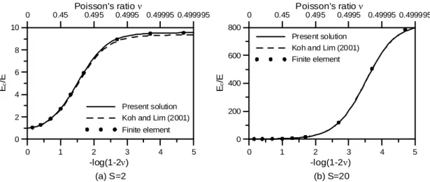
The effective compression modulus calculated from Eq. (40) by using the first 50 terms of the series is plotted as a function of Poisson’s ratio ν in Fig. 2 for the square layer

) 1 /

(a b= and in Fig. 3 for the rectangular layer of a/b=0.5 to compare with the finite element solution and the solution by Koh and Lim (2001). The square-layer solution of Tsai and Lee (1998) is also plotted in Fig. 2. These figures reveal that the present solution is very close to the finite element solution and the previous published results, which indicate that applying the approximate shear boundary conditions in Eqs. (15) and (16) to derive the effective compression modulus is acceptable.

To study the effect of aspect ratio, the ratio of the effective compression modulus of the rectangular layer in Eq. (40) to the effective compression modulus of the infinite-strip layer

) 0 /

(a b= in Eq. (42) is plotted in Fig. 4 as a function of aspect ratio for S =2 and S =20, which shows that the effect of the aspect ratio becomes significant only when Poisson’s ratio is close to 0.5. When Poisson’s ratio is small, the effective compression modulus has little

difference between the square layer (a/b=1) and the infinite-strip layer (a/b=0), if these bonded elastic layers have the same shape factor. Therefore, the solution of infinite-strip layer in Eq. (42) can be revised as

tanh )]

1 2 ( 1 1 1 [

1 ²

2 tS

tS E

E_c

α α ν

ν

ν + − ⁻

= − (44)

for the approximate solution of the rectangular layer. The range of Poisson’s ratio where Eq.

(44) is applicable is

1 for

2 . 0 5 .

0 − ¹ ≥

≤ S⁻ S

ν (45)

In this range, the error of the effective compression modulus calculated from Eq. (44) is smaller than 1.7%.

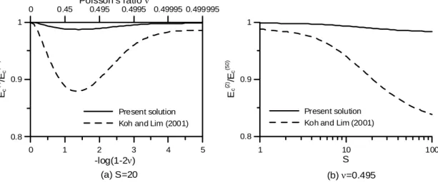
To study the convergence of the series solution in Eq. (40), let E_c^(k) denote the value of

E using the first k terms of the series in Eq. (40). Regarding c E_c⁽⁵⁰⁾ as the converged solution, the ratio of E to _c⁽¹⁾ E_c⁽⁵⁰⁾ is plotted in Fig. 5 for the rectangular layer of a/b=0.5 to depict the error of E . For the range of _c⁽¹⁾ 1≤ S≤100, the maximum error of E is about _c⁽¹⁾ 6%. The error of the solution by Koh and Lim (2001), which is also plotted in the figure, is lager than the present solution. Since the Koh-Lim solution is a double series form, E_c^(k) means the value of E which uses the first k terms in each series of the Koh-Lim solution, _c i.e., E_c^(k,k). As illustrated in Fig. 6, the maximum error of E_c⁽²⁾ for the present solution is about 2%. The error of the Koh-Lim solution plotted in this figure is higher than that reported in the paper of Koh and Lim (2001) where they mistook E_c^(2,10) for E_c^(2,2).

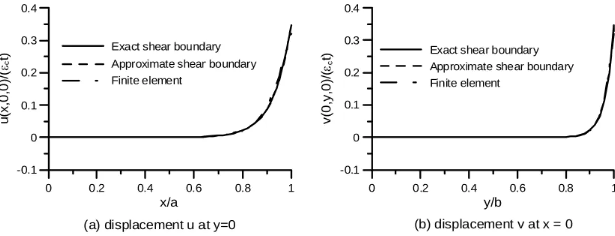
4. Solution of displacements

When using Eq. (8) to solve the displacement u(x,y), the pressure solution in Eq. (37) and the symmetric property of deformation imply that

] sin ) cosh cosh

cosh (

cos ) sinh sinh

sinh [(

) , (

1

x y

C y B

y A

y x

C x B

x A

y x u

n n

n n n

n n

n

n n

n n n

n n

γ γ

β δ

γ γ

β δ

+ +

+

+ +

= ∑^∞

= (46)

where A_n,B_n,C_n,A_n,B_n andC_n are the constants; the terms of A and_n A_n are the homogeneous solutions of Eq. (8), so that

2

2 12

n t

n = γ +

δ (47)

2

2 12

n t

n = γ +

δ (48)

Substituting Eqs. (37) and (46) into Eq. (8), the following constants can be solved as

n n n

n n c

n b a t

B t

γ β ν γ

ν β

ν ν ε ν

)] 1 ( 6

) 2 1 ( 1 3

cosh [ ) 1 ( ) 2 1 (

) 1 (

2 2 2

− +

− −

−

−

− −

= (49)

a b

C t

n n c

n ν γ

ε ν

cosh ) 1 ( ) 2 1 ( 2

2 −

= − (50)

)] 1 ( 6

) 2 1 ( 1 3

cosh [ ) 1 ( ) 2 1 (

) 1 (

2 2 2

ν γ

ν β

ν ν ε ν

− +

− −

−

−

= −

b t a

B t

n n

n c

n (51)

b a

C t

n n c

n ν γ

ε ν

cosh ) 1 ( ) 2 1 ( 2

2 −

− −

= (52)

from which, the boundary condition in Eq. (13) gives

n n n

n n c

n b a t

A t

δ γ ν γ

ν δ

ε ν

)] 1 ( 6 1 6

cosh [ ) 1 (

2 ^{2 2}

2

− + +

= − (53)

When using Eq. (9) to solve the displacement v(x,y), the pressure solution in Eq. (37) and the symmetric property of deformation imply

] cos ) sinh sinh

sinh (

sin ) cosh cosh

cosh [(

) , (

1

x y

F y E

y D

y x

F x E

x D

y x v

n n

n n n

n n n

n n

n n n

n n

γ γ

β δ

γ γ

β δ

+ +

+

+ +

= ∑^∞

= (54)

where D_n,E_n,F_n,D_n,E_n andE_n are the constants; the terms of D and_n D_n are the homogeneous solutions of Eq. (9). Substituting Eqs. (37) and (54) into Eq. (9), the following constants can be solved as

)] 1 ( 6

) 2 1 ( 1 3 cosh [

) 1 ( ) 2 1 (

) 1 (

2 2 2

ν γ

ν β

ν ν ν ε

− +

− −

−

−

= −

t a

b E t

n n

n c

n (55)

a b

F t

n n c

n ν γ

ε ν

cosh ) 1 ( ) 2 1 ( 2

2 −

− −

= (56)

n n n

n n c

n a b t

E t

γ β ν γ

ν β

ν ν ε ν

)] 1 ( 6

) 2 1 ( 1 3

cosh [ ) 1 ( ) 2 1 (

) 1 (

2 2 2

− +

− −

−

−

− −

= (57)

b a

F t

n n c

n ν γ

ε ν

cosh ) 1 ( ) 2 1 ( 2

2 −

= − (58)

from which, the boundary condition in Eq. (14) gives

n n n

n n c

n a b t

D t

δ γ ν γ

ν δ

ε ν

)] 1 ( 6 1 6

cosh [ ) 1 (

2 ^{2 2}

2

− + +

= − (59)

The remaining constants A and _n D could be solved by substituting Eqs. (46) and (54) _n