國
立
交
通
大
學
資訊科學與工程研究所
碩
士
論
文
繪圖處理器中順序獨立透明畫素片段儲存系統之設計
Transparent Fragment Storage System for Order-Independent
Transparency in GPU
研 究 生:林慧榛
指導教授:單 智 君 教授
繪圖處理器中順序獨立透明畫素片段儲存系統之設計
Transparent Fragment Storage System for Order-Independent
Transparency in GPU
研 究 生:林慧榛
Student:Hui-Chen Lin
指導教授:單智君
Advisor:Jyh-Jiun Shann
國 立 交 通 大 學
資 訊 科 學 與 工 程 研 究 所
碩 士 論 文
A Thesis
Submitted to Institute of Computer Science and Engineering
College of Computer Science
National Chiao Tung University
in Partial Fulfillment of the Requirements
for the Degree of
Master
In
Computer Science
August 2007
Hsinchu, Taiwan, Republic of China
繪圖處理器中順序獨立透明畫素片段儲存系統之設計
學生:林慧榛 指導教授:單智君 教授 國立交通大學資訊科學與工程研究所 碩士班摘 要
為了能正確且迅速繪製出場景透明度的效果,現今電腦圖學領域中提出
了順序獨立透明計算之演算法,並配以額外透明畫素片段儲存系統之支
援,以進一步降低演算法所需執行時間。然而,隨著現今對於高畫質場景
的要求愈來愈高的情況下,場景中具透明度像素片段之數目亦日漸增加,
其所需儲存空間亦日漸增大。如何能降低該儲存容量之需求,成為值得研
究之議題。本論文針對順序獨立透明計算,提出一畫素片段儲存系統之設
計:依畫素片段之螢幕座標位置,將畫素片段擺放至儲存系統中相對應的
位址,並利用指標索引方式,將具相同螢幕座標之畫素片段串連起來,達
到節省系統儲存空間、降低對儲存系統存取之次數、快速存取同螢幕座標
畫素片段及之目的。
Transparent Fragment Storage System for Order-Independent
Transparency in GPU
Student:Hui-Chen Lin Advisor:
Jyh-Jiun Shann
Institute of Computer Science and Engineering National Chiao-Tung University
Abstract
In order to correctly and fast render the transparent effect of a scene, some
hardware oriented algorithms with additional transparent fragment storage
supports for order-independent transparency are proposed in current computer
graphics. However, as the scene complexity is constantly increasing, the number
of transparent fragments and the size of transparent fragment storage support
also increase significantly. To lower the demand for memory, in this thesis, we
propose a transparent fragment storage system design for order-independent
transparency. Within our fragment storage system, transparent fragments are
stored in a corresponding location based on their x-y coordinate, and connected
with the other fragments that has the same x-y coordinate by pointer indexing.
The objective of our design is to reduce the memory requirement and the
memory access frequency of the transparent fragment storage system.
誌謝
這一年來的碩士研究生涯中,首先,我要感謝我的指導教授 單智君老師。感謝她 細心與極具耐心的指導,使我在我碩士研究中,直接由與單老師的討論中,獲得許多寶 貴的建議與方向,並且學習到如何以巨觀與微觀角度兼具地去看待研究事物,而得以完 成此碩士論文及順利通過畢業口試。我亦感謝同實驗室的另一位指導教授 鍾崇斌老 師,在鍾老師的諄諄教誨下,我習得參與群體討論、勇於提問的重要性,並且學習到如 何更客觀去評論研究事物、注意細節,對於我往後學習態度上,影響甚鉅。此外,感謝 我的畢業口試委員 林正中教授、邱日清教授、陳青文教授,由於他們的建議,使得此 論文研究更加完整。 同時,我也要感謝實驗室的學長姐、同學及學弟們在研究方面,給我很大的幫助。 特別謝謝惠親學姐辛苦地帶領與指導及討論、元化學長的關心與鼓勵、喬偉豪學長的建 議與幫忙,以及吳奕緯學長對於機器上維護付出的心力;謝謝GPU同組參與討論的同學們 相互打氣與支持,康康在實作上的幫忙及給予不錯的意見、辰瑋與立傑在討論中細心的 指正與建議;另外,亦要感謝順傑與柏駿等擔任實驗室系統維護的學弟們,在維修機器 及系統維護上的大力幫忙。沒有你們的幫助,我也無法如此順利地完成此碩士論文。 此外,我要特別感謝我親朋好友們給我的支持,謝謝小黃、軟哥、stephon等,在 程式實作上給與很大的指導與幫助; 小瞇、小豆、kano、stray給我不少鼓勵及幫助我 壓力的紓解; 還有天兵學長每天早上元氣的問候,使得我精神上振奮不少; 噢,我還要 特別感謝我男友ken,要不是他這麼努力地將自己吃得胖嘟嘟的,我也沒辦法有這麼溫暖 的懷抱可以依靠。最後,感謝我的家人在背後默默的支持我,即使你們對於研究上沒辦 法給予我太多意見,但有你們在一旁關心我,也讓我能更堅定與堅毅地繼續我的研究之 路。 所有陪我走過這段研究歷程的師長與親友們,謝謝你們這一路來的支持與鼓勵,謝 謝。 林慧榛 2007.8Table of Contents
摘 要 ...i
Abstract ...ii
誌謝 ...iii
Table of Contents ...iv
List of Figures ... v
List of Tables ...vi
Chapter 1 Introduction ... 1
Chapter 2 Background and Related work... 3
2.1 Graphics pipeline... 3
2.2 Transparency and alpha blending... 4
2.3 Transparency rendering problem ... 5
2.4 Order-independent transparency... 6
2.5 Related works... 7
2.5.1 R-Buffer hardware architecture... 7
2.5.2 Hardware oriented algorithm based on weight factors computations ... 9
Chapter 3 Design... 14
3.1 Design overview ... 14
3.2 Transparent Fragment Storage System ... 15
3.2.1 Statistics and observation for the distribution of transparent fragment... 15
3.2.2 The structure of transparent fragment storage system... 17
3.2.3 The access process of transparent fragment storage system ... 20
3.3 Leading 0s elimination ... 23
3.3.1 Statistics and observation of fragment data length ... 23
3.3.2 Main idea of leading 0s elimination ... 25
3.3.3 Example of leading 0s elimination ... 27
Chapter 4 Evaluation Results ... 28
4.1 Evaluation environment... 28
4.2 Test frame data ... 30
4.3 Simulation results ... 31
4.3.1 Memory requirement ... 31
4.3.2 time requirement ... 35
Chapter 5 Conclusion and Future Work ... 39
5.1 Conclusion ... 39
5.2 Future work... 39
References... 41
List of Figures
Figure 2-1 3D graphics pipeline... 3
Figure 2-2 Example of fragment blending processing ... 5
Figure 2-3 R-buffer graphics architecture scheme ... 8
Figure 2-4 R-buffer high level algorithm ... 9
Figure 2-5 Generic structure of WF hardware oriented algorithm... 10
Figure 2-6 WF hardware oriented algorithm... 11
Figure 3-1 the design diagram of transparent fragment storage system... 15
Figure 3-2 frame in DOOM3 ... 16
Figure 3-3 number of transparent fragments per pixel expressed by grayscale image ... 17
Figure 3-4 statistics of the number of transparent fragments per pixel... 17
Figure 3-5 diagram of SSA Table... 18
Figure 3-6 the structure of T-buffer ... 19
Figure 3-7 diagram of NSA Table ... 20
Figure 3-8 flowchart of the process for storing fragments into TFSS... 21
Figure 3-9 flowchart of the process for reading fragments from TFSS ... 22
Figure 3-10 distribution of the number of leading 0s of fragments ... 23
Figure 3-11 the number of leading 0s of fragments after multiplied by alpha value ... 24
Figure 3-12 cumulative percentage curves of transparent fragments... 25
Figure 3-13 transparent fragment storage system with leading 0s elimination... 26
Figure 3-14 example of leading 0s elimination... 27
Figure 4-1 simulation flow and ATTILA architecture... 28
Figure 4-2 a frame appearing in QUAKE4 ... 29
Figure 4-3 memory requirement comparison... 32
Figure 4-4 average memory reduction rate of TFSS ... 33
Figure 4-5 memory requirement comparison... 34
Figure 4-6 average memory reduction rate of TFSS with leading 0s elimination ... 35
Figure 4-7 execution time comparison... 37
Figure A-1 frame60... 43
Figure A-2 frame120... 43
Figure A-3 frame180... 44
Figure A-4 frame240... 44
Figure A-5 frame300... 45
Figure A-6 frame360... 45
Figure A-7 frame420... 46
List of Tables
Table 4-1 statistics of test frames... 30 Table 4-2 memory requirements of each of transparent storage systems ... 32
Chapter 1 Introduction
In order to support realistic scene in computer graphics, a special purpose processor, called Graphics Processing Unit or GPU, is required for high performance 3D graphics rendering. As the demand for high quality realistically rendering in computer graphics is continuously increasing, the support for transparent effect becomes more important for visual reality. Current GPUs provide the capability to generate the effect of transparency. The operation implemented in GPU to generate the transparent effect is called alpha blending: combining a translucent foreground with a background. Due to the alpha blending operation, rendering a scene with transparent objects realistic requires rendering in correct depth order— from back to front or front to back with respect to the viewpoint. It implies that the rendering order of transparent objects depends on their depth order with respect to the viewpoint, that is, order-dependent transparency. Traditionally, the transparent objects are sorted to get the correct depth order in the application level. However, it is difficult for software application developers to sort transparent objects since objects may intersect each other. In addition, as the number of transparent primitives increases rapidly, the application sorting becomes more and more complicated. Therefore, order-independent transparency, rendering transparent objects without application depth sorting, becomes an important issue for high performance rendering systems.
Order-independent transparency is a difficult architectural problem to solve and many researches have been investigated on it. There are several different kinds of order-independent transparency algorithms. Some algorithms model the alpha value as a probability measure such as alpha-dithering [Will]. Other multi-pass rendering algorithms [Ever01] pass fragments several times to blend them and produce the correct results. For the reason of fast rendering, most order-independent transparency algorithms modified the traditional GPU architecture
with the additional hardware support for storing these transparent fragments. R-buffer(RB) proposal [Witt01] implements A-buffer [Carp84] software algorithm into hardware by adding an extra storage system to store transparent fragments in their arrival order. WF (Weight Factor) hardware oriented algorithm [Amor06] precomputes the contribution factor of each fragment to the final color of a pixel and sequentially stores transparent fragments based on their x-y coordinate into storage system.
As the scene complexity arises, the number of transparent fragments and the storage space for transparent fragments increase significantly. How to store these transparent fragments to lower the demand for memory becomes more and more important. In addition, current fragment storage support techniques for order-independent transparency [Amor06] [Witt01] still have some defects to be improved such as large storage requirement and high memory access frequency. Therefore, our objective is to design a transparent fragment storage system which places order-independent-arrival transparent fragments in such an organized way that reduces the memory requirement and memory access frequency in comparison with previous works. In addition, for the purpose to further reduce the memory requirement of proposed transparent fragment storage system, we also use leading 0s elimination technique to strip the redundant part of fragment data.
The rest of this thesis is organized as follows: In Chapter 2, we introduce an overview of graphics pipeline, transparency rendering operation and problem, and related works of fragment storage system for order-independent transparency. In Chapter 3, we propose the design of our transparent fragment storage system and the utilization of leading 0s elimination technique. In Chapter 4 we discuss and show our simulation environment and results. In chapter 5, we summarize our conclusions and future work.
Chapter 2 Background and Related work
In this chapter, we will give an overview of graphics pipeline. Then, we will introduce the definition of transparency, alpha blending operation, explain the transparency rendering problem, and expatiate on order-independent transparency. At the end of this chapter, we will present the details of two previous works related to hardware support techniques for order-independent transparency.
2.1
Graphics pipeline
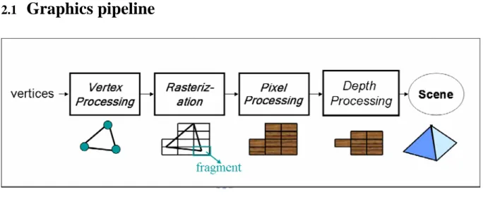
Figure 2-1 3D graphics pipeline
Graphics pipeline can be roughly divided into four stages: vertex processing,
rasterizarion, pixel (fragment) processing, and depth processing, as shown in Figure 2-1.
At vertex processing stage, vertices undergo coordinate transformation, lighting, and clipping operations. After vertex processing stage, these calculated vertices are sent into rasterization stage, which consists of two parts. The first part, called triangle setup, is to combine three vertices into a triangle, and the second part is to determine which squares of an integer grid in screen coordinate are occupied by the triangle and to assign a color and a depth value to each such square. Such generated image square is called fragment, which is defined as a pre-pixel before being sent to a screen. Fragments are then sent into pixel processing stage. At pixel
processing stage, the color of fragments are calculated based on values interpolated from the vertices or determined by texture mapping [Watt00]. Finally, fragments occluded by other fragments and invisible at the final screen are discarded at depth processing.
The graphics pipeline is implemented on GPUs, designed with high parallel structure which makes it more efficient than CPU, and the two describe stages —vertex processing and pixel processing— are implemented as programmable stages, named vertex shading and pixel shading, on GPUs..
Since our system is designed for storing fragments, which are generated after rasterization; therefore, we are only concerned about the process between rasterization stage and pixel processing in graphics pipeline in this thesis.
2.2
Transparency and alpha blending
Translucent objects can be rendered by specifying the degree of transparency with a color. The value to represent the degree of transparency is defined as an alpha (α) value, which ranges from 0.0(completely transparent) to 1.0(completely opaque). Each fragment has its alpha value with its RGB color components. To obtain the final color of a pixel, the translucent fragments belonging to the pixel (i.e., fragments have the same x-y coordinate) are typically assumed to be rendered from back to front in visibility order, or depth order. The process of blending a translucent foreground with a background color to generate the effect of transparency is called alpha blending. Normally, the alpha blending equation (1) [Port84] is used for alpha blending, as shown below:
b f f
fc c
c=α +(1−α ) Eq. (1)
, where c is the final color of a pixel, c and f αf are the color and the alpha value of foreground transparent fragment, and c is the color of background fragment. b
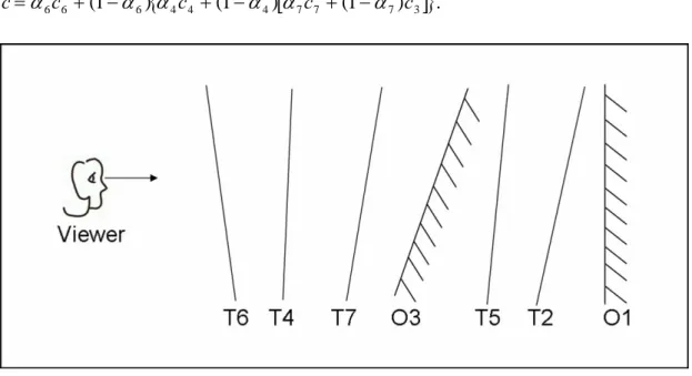
To clarify, consider an example shown in Figure 2-2. In Figure 2-2, six fragments are belonging to the same pixel, two of them are opaque (O1 and O3) and four of them are transparent (T2, T4, T5, T6, and T7). The suffixes of fragments indicate the sequential order where the fragments are received. The fragments are viewed from the left. The final color of the pixel is obtained by the combination of the closest opaque fragment O3 and the blending result of the transparent fragments processing from back to front: first T7, second T4 and finally T6. That is, assume ci and αi represent the color and the alpha value of fragments, where i is fragment’s received order, according to Eq. (1), the final color c of the pixel is equal to
[
]
{
4 4 4 7 7 7 3}
6 6 6c (1 ) c (1 ) c (1 )c c=α + −α α + −α α + −α .Figure 2-2 Example of fragment blending processing
2.3
Transparency rendering problem
The blending equation (1) is order-dependent, which means that transparent fragments require to be processed in their depth order, not in their arrival order. Thus, if we render transparent fragments in arbitrary order, it will produce an artificial result. For example, in Figure 2-2, fragment T4 and T6 come before fragment T7, if we blend T4 and T6 with opaque
fragment O3 first, the blend T7 later, according to Eq. (1), the final color c will be
[
]
{
}
3 4 6 7 4 4 6 7 6 6 7 7 7 3 4 4 4 6 6 6 7 7 7 ) 1 )( 1 )( 1 ( ) 1 )( 1 ( ) 1 ( ) 1 ( ) 1 ( ) 1 ( c c c c c c c c c α α α α α α α α α α α α α α α − − − + − − + − + = − + − + − + =But the correct final color should be
[
]
{
}
3 7 4 6 7 7 4 6 4 4 6 6 6 3 7 7 7 4 4 4 6 6 6 ) 1 )( 1 )( 1 ( ) 1 )( 1 ( ) 1 ( ) 1 ( ) 1 ( ) 1 ( c c c c c c c c c α α α α α α α α α α α α α α α − − − + − − + − + = − + − + − + =Thus, the incorrect result is produced due to the incorrect rendering order.
Since fragments are generated in arbitrary order at rasterization, not in depth order, several algorithms are proposed for correct transparent rendering. These algorithms can be classified as sorting based algorithms and order-independent transparency algorithms. Sorting based algorithms require the primitives (polygons) to be sorted from back to front with respect to the viewpoint. These sorting algorithms can further be classified into application sorting [Mamm89, Snyd98], hardware assistant sorting [Ever01], and hardware sorting [Amor06, Winn97] algorithms based on the method they use to sort the primitives. However, for application sorting algorithms, it is difficult to do depth sorting since objects in a scene may intersect each other and intersected parts need to be divided into several polygons. Even for those hardware assistant sorting algorithms, it is very time-consuming. Therefore, it comes out order-independent transparency.
2.4
Order-independent transparency
Order-independent transparency is defined as a process which renders transparent fragment in arbitrary order instead of sorting them in advance. There are several different kinds of order-independent transparency algorithms.
Some algorithms model the alpha value as a probability measure such as alpha-dithering [Will] [Muld98], or alpha-to-coverage. These algorithms sample the alpha value and interpret
it as how much it covers the pixel to produce dithering-like transparent effect in images. These algorithms are single-pass rendering, do not require depth sorting, and do not handle intersected polygons in advance. However, since they are probability-measure algorithms, they also have chance to produce artificial results. Other order-independent transparency algorithms [Ever01] use multi-pass rendering method to process transparent fragments several times that render them in correct depth order. These multi-pass rendering algorithms are some kinds of fragment-level depth sorting technique; therefore, in general cases, they have the same defect as sorting algorithms have, that is, time consuming.
Thus, most order-independent transparency algorithms modified the traditional GPU architecture to solve time-consuming problem. Z3 hardware technique [Joup99] is one of these modified hardware architecture which only renders a fixed number of transparency layers correctly. R-buffer(RB) [Witt01] is a modified hardware architecture which implements A-buffer [Carp84] software algorithm into hardware by adding an extra storage system to store transparent fragments associated with each pixel. WF (Weight Factor) hardware oriented algorithms [Amor06] precomputes the contribution factor of each fragment to the final color of pixel and propose an organized strategy to sequentially store transparent fragments corresponding to the same pixel. Since our research focuses on hardware storage support for order-independent transparency, we will introduce more details of R-buffer hardware architecture and WF hardware oriented algorithm, which are more related to our system design.
2.5
Related works
2.5.1 R-Buffer hardware architecture
R-buffer (RB) [Witt01] is a graphics hardware architecture which implements A-buffer software algorithm [Carp84]. Figure 2-3 shows the R-buffer graphics architecture. The
R-buffer architecture is a standard graphics pipeline with additional hardware support: a proposed recirculating fragment buffer, called R-buffer, pixel state memory, and a second z-buffer. In rasterization stage, the objects are rasterized into fragments in arbitrary depth-order. After rasterization, a transparent fragment is sent to the R-buffer, and the depth value of an opaque fragment is compared with the depth value in z-buffer to find the closest opaque fragment which needs to be placed into frame buffer. The transparent fragments behind the closest opaque one are discarded. Then, each transparent fragment in R-buffer is read out iteratively to find the furthest one to be blended with the fragment in frame buffer.
Figure 2-3 R-buffer graphics architecture scheme [Witt01]
Figure 2-4 shows the high level R-buffer algorithm. Phase 1 rasterizes the primitives into fragments and places the closest opaque fragment into frame buffer, the furthest transparent fragment’s depth value into second z-buffer. Phase 1 is equivalent to early z test with the exception that unoccluded transparent fragments are sent into R-buffer and second z-buffer is updated with the depth value of the furthest visible transparent fragment. After all fragments are generated, in phase2, the transparent fragments in R-buffer are discarded if they are occluded by the opaque fragments in frame buffer. If the R-buffer is not empty, the phase3 is
processed iteratively to find the transparent fragment whose depth value matches the depth in the second z-buffer from R-buffer and blend that transparent fragment with the fragment in frame buffer, and then, drop that transparent fragment from R-buffer. When the R-buffer is empty, the whole process is finished.
Figure 2-4 R-buffer high level algorithm [Witt01]
The R-buffer is a FIFO (first-in-first-out) memory which stores transparent fragments in the sequence that they arrive. The information of each transparent fragment —the location (x, y), the depth value (z), the color value (RGB) with alpha value(A or α)— needs to be stored in the R-buffer. Pixel state memory stores each pixel’s current state. The second z-buffer stores the depth value of the furthest visible transparent fragments per pixel. The memory size of the R-buffer is proportional to the number of transparent fragments after early z test. The memory size of the second z-buffer is equivalent to the original z-buffer. In pixel state memory, each pixel needs three bits to record its current value; thus, the memory size of the pixel state memory is equal to three multiplied by the screen size. To sum up the memory requirement of R-buffer architecture, we list the R-buffer memory requirement equation as follow:
Memorytotal = MR-buffer + M2nd-z-buffer + Mstate-memory
2.5.2 Hardware oriented algorithm based on weight factors computations
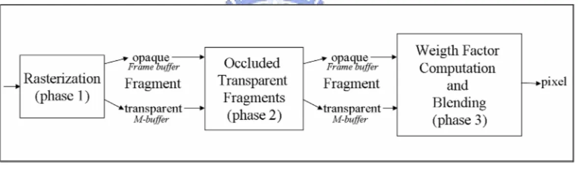
Factor) hardware oriented algorithm in brief. WF hardware oriented algorithm is based on the precomputation of the contribution of each fragment to the final color of the pixel with the specialized storage scheme. Figure 2-5 shows the generic structure of WF hardware oriented algorithm. Phase 1 and phase 2 of WF hardware oriented algorithm are similar to those of R-buffer high level algorithm, shown in Figure 2-4. In phase 1, fragments are sequentially generated and the current closest opaque transparent is placed into frame buffer while the transparent fragments are stored into another buffer, called Mbuffer. In phase 2, all transparent
fragments stored in Mbuffer are analyzed and discarded if they are occluded by the closest
opaque fragment stored in frame buffer. In phase 3, each transparent fragment in Mbuffer is
compared with other fragments belonging to the same pixel in order to compute its weight factor and the blending of the fragment is performed.
Figure 2-5 Generic structure of WF hardware oriented algorithm
The weight factor computation is based on the analysis of the blending equation (1). By breaking the recursivity of the blending equation (1), the equation can be revised as:
∑
= = n i i i i c w c 0 α Eq. (2), where there are n transparent fragments and one opaque fragment belonging to the pixel which has the final color c, c is the color of the transparent fragment i,i αi is the alpha value of fragment i, and w is the weight factor of the transparent fragment i. The weight factor i
i
w is computed by the accumulative contribution of all transparent fragments j in front of the
∏
= = n j j i a w 0 Eq. (3) with ⎩ ⎨ ⎧ − < = otherwise. 1 Z if 1 j j i j Z a α Eq. (4)Figure 2-6 WF hardware oriented algorithm
The WF hardware oriented algorithm is outlined in Figure 2-6. It can be basically divided into three stages: SETUP (line 1-6), OCCLUDED TRANSPARENT FRAGMENTS (line 9-12), WEIGHT FACTOR COMPUTATION (line 14-22). Assume that there are n+1 fragments are processed sequentially to the same pixel. In SETUP stage, if a fragment is transparent, it is placed into Mbuffer; otherwise, if a fragment is opaque and closest to the view
point at the time, it is stored into frame buffer and Z-buffer is updated by its depth value. Note that some transparent fragments are visible when they are compared to the front-most opaque fragment at the time they arrive, but a closer opaque fragment may arrive later and occlude them. Therefore, in the second stage, OCCLUDED TRANSPARENT FRAGMENTS, those transparent fragments in Mbuffer are discarded for the reason that they are occluded by the
closest opaque fragment. In the last stage, WEIGHT FACTOR COMPUTATION, each fragment is compared with all those following in the Mbuffer in order to compute its weight
factor. Obviously, these three stages in Figure 2-6 are the same as the three phases in Figure 2-5.
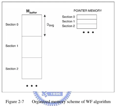
Figure 2-7 Organized memory scheme of WF algorithm
The organized memory scheme of WF algorithm is shown in Figure 2-7. It suggests that transparent fragments belonging to the same pixel are stored sequentially and connectedly in the Mbuffer. Mbuffer is organized in sections of Davg words, where Davg is the average number of
fragments per pixel. Each pixel has it corresponding storage section, with capacity for Davg
fragments; that is, for a system with W×H pixels, W×H sections would be required and a pixel i in a system has a corresponding section i in Mbuffer. To extend the storage capabilities, a
pointer memory is added so that more than one section can be dynamically assigned to a given pixel. The information stored per section of a pointer memory indicates that whether one section is sufficient (by storing a NULL pointer) or whether the following-coming fragments are stored in another section (by storing the section index). For example, if there
are F transparent fragments belonging to a pixel i, where F is larger than Davg, the first Davg
fragments are stored in section i of Mbuffer, and the following F- Davg fragments are stored in
another section j (j ≧ W×H). The section i of a pointer memory stores the section j index. If
section j is still insufficient to store F- Davg fragments (i.e., F- Davg > Davg), the rest F-2×Davg
Chapter 3 Design
In this chapter, our transparent fragment storage system is proposed. The objective of our transparent fragment storage system is to reduce the memory requirement and memory access of transparent fragments for order-independent transparency. In addition, we also propose a leading 0s elimination technique to compress fragment data size and further reduce the memory requirement of the proposed transparent fragment storage system. This chapter is organized as follows: in section 3.1, the system design overview is introduced; in section 3.2 our transparent fragment storage system is proposed; in the last section of this chapter (section 3.3), we present the leading 0s elimination technique.
3.1
Design overview
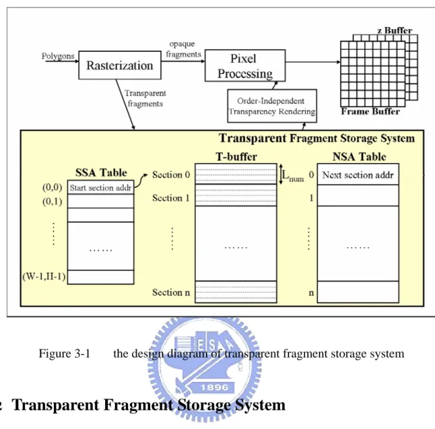
The overview of our proposed transparent fragment storage system is shown in Figure 3-1. There are three components in our transparent fragment storage system: start-section
address table (SSA Table), T-buffer, and next-section address (NSA Table). After rasterization stage, the polygons are segmented into several fragments in arbitrary order. Then, opaque fragments continue the pixel processing procedure while transparent fragments are stored into our transparent fragment storage system (TFSS). The details of our transparent fragment storage system will be introduced in section 3.2. In addition, we also design leading
0s elimination, which is the process that reduces a fragment data size by eliminate the leading 0s of fragment’s color components (RGB). The details of leading 0s elimination will be introduced in section 3.3.
Figure 3-1 the design diagram of transparent fragment storage system
3.2
Transparent Fragment Storage System
3.2.1 Statistics and observation for the distribution of transparent fragment
Figure 3-2 shows a frame image in DOOM3. We analysis the number of transparent fragments of each pixel in this frame and obtain the result in Figure 3-3 and Figure 3-4. Figure 3-3 is a gray-level image, and black color indicates that the number of transparent fragments of a pixel is 0, while white color indicates that the number of transparent fragments of a pixel is 7, that is, the maximum number of transparent fragments of a pixel in the frame. The transparent fragment numbers of a pixel between 0 and 7 and their corresponding colors are shown at right side of Figure 3-3. More detail of statistics of the transparent fragment number in the frame is shown in Figure 3-4. We find that not all pixels in a frame have
transparent fragments. However, in WF proposal, each pixel is assigned the same size of memory space, no matter whether the pixel has transparent fragments or not. Thus, if we use a transparent storage support proposed in WF proposal, it needs a large memory space and parts of them are unused resulting in unnecessary memory cost.
Figure 3-3 number of transparent fragments per pixel expressed by grayscale image 0 50,000 100,000 150,000 200,000 250,000 300,000
The number of transparent fragment per pixel
T h e num b e r of pi xel s 0% 20% 40% 60% 80% 100% T h e c u mu la tiv e p e rc e n ta g e (%)
the number of pixels cumulative percentage of pixel number the number of pixels 266,978 28,818 6,387 3,637 1,145 234 1 cumulative percentage of pixel
number
86.91% 96.29% 98.37% 99.55% 99.92% 100.00% 100.00%
0 1 2 3 4 5 6
Figure 3-4 statistics of the number of transparent fragments per pixel
3.2.2 The structure of transparent fragment storage system
the design diagram of transparent fragment storage system (TFSS) is shown in Figure 3-1. The storage scheme of TFSS is to store transparent fragments in an organized way based on their coordinate; that is, transparent fragments belonging to a pixel are stored serially in TFSS. The transparent fragment storage system (TFSS) is composed of three components: SSA Table, T-buffer, and NSA Table. The structure and the function of each component in TFSS will be described in 3.2.2.1 to 3.2.2.3.
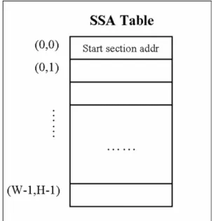
3.2.2.1 SSA(Start-Section Address) Table
Figure 3-5 diagram of SSA Table
As shown in Figure 3-5, SSA Table has W times H entries, where W is defined as the width of a screen, and H is defined as the height of a screen. Each pixel p in a screen has a corresponding entry ep in SSA Table and each entry in SSA Table stores the address of start
section for pixel p. Namely, pixel p has assigned the entry ep in SSA Table. If a pixel does not
have the start section— the pixel does not have transparent fragments— a nullified address is stored in the corresponding entry in SSA Table.
3.2.2.2 T-Buffer
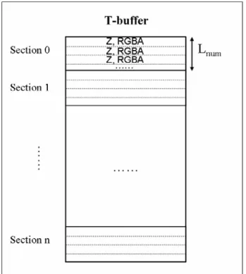
T-buffer is a storage space for transparent fragments. As shown in Figure 3-6, T-buffer is organized in sections of Lnum, where Lnum represents the maximum number of transparent fragments that can be stored in a section. Each section stores transparent fragments with the same x-y coordinate; that is, fragments belonging to the same pixel are stored gregarious within one section in T-buffer. There might be more than Lnum transparent fragments which have the same x-y coordinate. Thus, more than one section should be assigned to a pixel to extend the capability for storing variable number of fragments. We use NSA Table to record the address of next section which is assigned to store the following fragments.
Figure 3-6 the structure of T-buffer
3.2.2.3 NSA(Next-Section Address) Table
capable of storing, the excess fragments will be stored in another section. Then, the address of the section is recorded as the next-section address in NSA Table. Figure 3-7 shows the diagram of NSA Table. The number of entries in NSA Table is equivalent to the number of sections in T-buffer and there is a one-to-one correspondence between entries in NSA table and sections in T-buffer. However, if one section is sufficient to store transparent fragments of a pixel, there is no need to assign another section, and thus, the NULL pointer is stored instead of the section address.
Figure 3-7 diagram of NSA Table
3.2.3 The access process of transparent fragment storage system
In this section, the access process of transparent fragment storage system is described. The process for storing fragments into TFSS is described in 3.2.3.1; the process for reading fragments from TFSS is described in 3.2.3.2.
3.2.3.1 The process for storing transparent fragments into TFSS
the address of start section s(i,j) is read from the corresponding entry e(i,j) in SSA Table. If s(i,j)
of T-buffer, the start section, is full, the address of next section ns which is available (not full)
for storing fragments is read from the entry es of NSA Table. After the address of section ns is obtained, the fragment is eventually stored into section ns of T-buffer. If there is no start
section or no next section for a given pixel, the new empty section in T-buffer is assigned for that pixel, and the address of the new section is recorded in SSA Table as the start-section address or in NSA Table as the next-section address for the pixel. Figure 3-8 shows the flowchart of the process for storing fragments into TFSS.
3.2.3.2 The process for reading transparent fragments from TFSS
For each pixel p(i,j ) in a screen, the start-section address is read from its corresponding entry e(i,j) in SSA Table. If there is no start-section address for a pixel, the process is continued to read the start-section address from the next entry e(i,j+1) for the next pixel. Otherwise, transparent fragments belonging to p(i,j ) are accessed from the start section s(i,j) of T-buffer and the address of next section ns can be read simultaneously from the entry s of NSA Table.
If there is no next section for p(i,j ), instead, the NULL is stored in entry s of NSA Table, the process is continued for the next pixel. Otherwise, the fragments in the next section n are accessed from T-buffer and the address of the next section n’ of section n can be looked up simultaneously from the entry n of NSA Table. This process is recursively done until there is no next section for pixel (xi,yi). Figure 3-9 shows the flowchart of the whole process for
reading fragments from TFSS.
3.3
Leading 0s elimination
3.3.1 Statistics and observation of fragment data length
0 10000 20000 30000 40000 50000 60000 70000 0 1 2 3 4 5 6 7 number of leading 0s num be r of t ra ns pa re nt f ra gm en ts 0% 20% 40% 60% 80% 100% R G B
cumulative percentage of R cumulative percentage of G cumulative percentage of B
Figure 3-10 distribution of the number of leading 0s of fragments
Figure 3-10 shows the distribution of the number of leading 0s of fragments before multiplied by alpha value in frame130. In Figure 3-10, the horizontal axis represents the number of leading 0s of a fragment, ranging from 0 to 7 for each 8-bit color component; the vertical axis represent the number of transparent fragments. The yellow, light blue, and purple curves in Figure 3-10 represent the cumulative percentage of fragments in accordance with the number of leading 0s. As we can see, about 80% fragments, their effective value of each color component only use less than 4 bits.
When RGB color components of a fragment are multiplied by fragment’s alpha value, the number of leading 0s of each of RGB color components will increase, as shown in Figure 3-11. This phenomenon gives us a thought that it does not need full 8-bit memory space to
store each color component of a transparent fragment; that is, we can eliminate leading 0s of each color component of a transparent fragment before it is stored into T-buffer to further reduce the memory requirement of transparent fragment storage system.
0 20,000 40,000 60,000 80,000 100,000 120,000 140,000 160,000 0 1 2 3 4 5 6 7 number of leading 0s num be r of t ra ns par ent fra gm en ts 0% 20% 40% 60% 80% 100% cum ul at ive pe rce nt age (% ) R G B
cumulative percentage of R cumulative percentage of G cumulative percentage of B
Figure 3-11 the number of leading 0s of fragments after multiplied by alpha value
The original cumulative percentage curve of transparent fragments is compared with the cumulative percentage curve after multiplied by alpha value, as shown in Figure 3-12, where line1-R,G,B represent the former and line2-R,G,B represent the latter. Line3-R,G,B in Figure 3-12 represent the cumulative curve of transparent fragments when we choose the minimum number of leading 0s among RGB color components as the number of leading 0s of each color component. We observe that there is a little difference between line2 and line3, and it implies that perhaps a fixed-length leading 0s elimination to RGB color component of a fragment can achieve approximate memory reduction ratio as variable-length leading 0s elimination.
cumulative percentage curve
0%
20%
40%
60%
80%
100%
0
1
2
3
4
5
6
7
number of leading leading 0s
cu
m
ul
at
iv
e
per
cen
tag
e
of
tr
an
sp
ar
en
t
fr
ag
men
ts
(
%
)
line1-R
line1-G
line1-B
line2-R
line2-G
line2-B
line3-R
line3-G
line3-B
Figure 3-12 cumulative percentage curves of transparent fragments
3.3.2 Main idea of leading 0s elimination
According to the statistics and observation in 3.3.2, we decide to use a leading 0s elimination to further reduce the memory requirement for transparent fragments. Leading 0s elimination is a simple and quick process that eliminates the leading zero bits of three color component data(RGB) simultaneously until leading 1 occurs in any one of the three color components. Notice that we do not eliminate all leading zero bits from each color component, instead, we just eliminate the minimum number of leading 0s among RGB color components; that is, fixed-length leading 0s elimination for each RGB color component of a transparent fragment.
The operation of leading 0s elimination is simple. First, eliminate leading zero bits of three color components (RGB) simultaneously until leading 1 occurs in any one of the three
color components. Then, shift the RGB color component data to the right by several bits based on fragment’s alpha value. Finally, record the length of RGB color component after elimination.
As shown in Figure 3-13, for leading 0s elimination, an additional design component, called Length Table, is added into our transparent fragment storage system to support variable-length fragment data retrievals. Length Table records the length of RGB color components of a fragment after leading 0s elimination. There is a one-to-one correspondence between entries in Length Table and sections in T-buffer; that is, each entry in Length Table records the lengths of fragments in its corresponding section and each entry in Length Table can record at most Lnum lengths of fragments, where Lnum represents the maximum number of transparent fragment that can be stored in a section.
3.3.3 Example of leading 0s elimination
Figure 3-14 shows an example of leading 0s elimination. Assume that each color component of a fragment is 8 bits, fragment’s alpha value is 0.125, and the value of each color component is represented in binary format. First, the minimum number of leading 0s among RGB color components is two; thus, we eliminate two leading zero bits from each of three color components (RGB) simultaneously. Then, shift the RGB color component data to the right by 3 bits based on fragment’s alpha value. Finally, record the length of RGB color component after elimination.
Chapter 4 Evaluation Results
In this chapter, we first show our evaluation environment and the characteristic of input frame data (in section 4.1 and 4.2). Then, we show and analyze simulation results of memory requirement and execution time during rendering of each method: R-buffer, WF hardware oriented algorithm, and our TFSS design in section 4.3. In the last section, we briefly summarize our conclusion from the results.
4.1
Evaluation environment
Figure 4-1 shows the architecture of ATTILA simulator and when we dump trace of fragment data from ATTILA simulator for our simulator. We implemented a behavioral simulator of the architecture with the transparent fragment storage system in C++, and modified ATTILA simulator [Moya06] to output fragment information to a tracefile. The benchmark used in ATTILA simulator is QUAKE4 [Rave05], a modern graphics application. Figure 4-2 shows one frame appearing in QUAKE4. The tracefile outputted from ATTILA simulator contains the coordinates and RGBA color components of fragments in frames. Our simulator reads the tracefile and evaluates the memory requirement and access frequency time of transparent fragment storage system.
Figure 4-2 a frame appearing in QUAKE4
Display resolution: the number of distinct pixels in each dimension that can be displayed.
Color component bit-width: the bit-width of each of the RGBA color components Lnum : the maximum number of transparent fragments that a section in T-buffer can
stores.
Msection: the memory size of a section in T-buffer
In our simulator, we assume the display resolution is 640×480, the bit-width of each of RGBA color components is 8 bits, and modulate the value of Lnum and Msection to observe the memory requirements.
4.2
Test frame data
Table 4-1 statistics of test frames
In this section, we provide statistics of eight test frames, which are dumped at the interval of 60 frames, as shown in Table 4-1. In Table 4-1, the second column indicates the Frame
No. of pixels whose no. of transparent fragments = N N No. of fragments No. of transparent fragments No. of transparent fragments per transparent pixel Transparency density 1 2 3 4 5 Frame60 2,377,518 37,684 2.37 5% 5,812 956 6,633 2,279 189 Frame120 746,943 37,594 2.38 5% 5,723 956 6,634 2,278 189 Frame180 516,464 40,584 2.16 6% 8,713 956 6,634 2,278 189 Frame240 488,112 88,434 1.63 18% 32,588 12,040 7,235 2,279 189 Frame300 623,531 60,769 1.61 12% 26,082 2,729 6,636 2,179 121 Frame360 587,617 69,768 1.61 14% 27,421 7,094 7,006 1,569 173 Frame420 530,258 47,877 1.77 9% 15,728 3,290 6,770 1,296 15 Frame480 605,927 135,475 1.22 36% 95,226 8,716 6,711 671 0
total number of opaque and transparent fragments in each frame; the third column shows the number of transparent fragments in each frame; the fourth column shows the number of transparent fragments per transparent pixel; the fifth column shows the transparency density, which is defined as the percentage of transparent pixels in a frame (i.e. #transparent pixel/display resolution). The last column shows the distribution of transparent fragment layers per pixel in each frame. For example, in frame 120, 5723 pixels have 1 transparent fragment layer, 956 pixels have 2 transparent fragment layers, 6634 pixels have 3 transparent fragment layers, 2278 pixels have 4 transparent fragment layers, 189 pixels have 5 transparent fragment layers, and no pixel have more than or equal to 6 transparent fragment layers.
4.3
Simulation results
In this section, we show the simulation results of memory requirements and access frequency time of fragments storage system. We compare the results of our design with two related works: R-buffer and WF hardware oriented algorithm.
4.3.1 Memory requirement
In order to evaluate our transparent fragment storage system (TFSS), we compare our storage design with two related works: R-buffer [Witt01] and WF hardware oriented algorithm [Amor06]. We list the memory requirements of each method in Table 4-2. The second column shows the name and the size of a transparent fragment storage space in each technique and the third column shows the name and the size of other storage supports in each storage system. In Table 4-2, Nf is defined as the number of transparent fragments, NA is
defined as the number of dynamic allocated sections in WF algorithm, and NS is defined as the
number of sections in T-buffer in our design; Sf is defined as the size of a fragment data
section in M-buffer in WF algorithm, and MTFSS is defined as the memory size per section in
T-buffer in our TFSS; W and H are defined as the width and the height of a display screen. Transparent fragment storage system
transparent fragment memory other storage supports techniques
Name size Name Size
2nd Z buffer = Z buffer size (W×H×Z’s bytes) R-buffer R-buffer Nf×Sf
state memory 3(bits) ×W×H WF algorithm M-buffer (W×H+NA) ×MWF pointer memory SA × (W×H+NA)
SSA Table SA×W×H TFSS T-buffer MTFSS×NS
NSA Table SA×NS
Table 4-2 memory requirements of each of transparent storage systems
Based on the memory requirements listed in Table 4-2, we obtained the simulation result of memory requirement of each technique, as shown in Figure 4-3. We find that in average, our TFSS has the lowest memory requirement than two related works.
0 2 4 6 8 10 fram e60 fram e120 fram e180 fram e240 fram e300 fram e360 fram e420 fram e480 AVER AGE frame m emory si ze (M B ) RBUF WF(3) WF(2) WF(1) TFSS(3) TFSS(2) TFSS(1)
Figure 4-3 memory requirement comparison1
1
WF(Davg) represents WF algorithm has the capability for storing Davg fragments per section in M-buffer
Notice that in frame480, the memory requirements of our TFSS with Lnum=3 are larger than those of R-buffer technique. We conjecture that this result is occurred by the weakly utilization of a section, which has the capability for storing three transparent fragments but only stores fewer than three fragments. As shown in Table 4-1, the proportion of pixels which have one transparent fragment in frame480 is much larger than those in other frames. In fact, the percentage of pixels with one transparent fragment in frame480 is about 30%, while it is only 2% to 10% in other frames. It indicates that about 30% of sections in T-buffer are weakly utilized in frame480. Therefore, it results in unnecessary memory cost and larger memory requirement of TFSS with Lnum=3 than of R-buffer.
0% 10% 20% 30% 40% 50% 60% 70% 80% 90% RBUF WF(3) WF(2) WF(1)
fragment sotrage systems
m em or y re duc ti on rat e (% ) TFSS(3) TFSS(2) TFSS(1)
Figure 4-4 average memory reduction rate of TFSS
The average memory reduction rate of our TFSS is presented in Figure 4-4. As shown in Figure 4-4, our TFSS can achieve 18% to 41% memory reduction rate in comparison with R-buffer architecture, and 40% to 81% reduction rate in comparison with WF algorithms. It shows that our TFSS has great advantage over other related works.
Since the size of each fragment is reduced after leading 0s elimination, the memory size of each section within T-buffer in TFSS does not need as large as before. In our TFSS, without leading0s elimination, each section within T-buffer is Lnum×8bytes large (Figure 4-3). We suppose that with leading0s elimination, each section is smaller than Lnum×8bytes. Thus, we reduce the section size to evaluate the memory reduction ratio by leading 0s elimination. As we expect, the memory requirement of transparent fragment storage system will be further reduced by leading 0s elimination. We evaluate the memory requirement of our TFSS design with leading 0s elimination and compare the result with other related works, as shown in Figure 4-5. We notice that in each frame cases, including frame480, our design has the lowest memory requirement. 0 2 4 6 8 10 fram e60 frame1 20 fram e180 fram e240 fram e300 fram e360 frame 420 frame4 80 AVER AGE frame m em ory s iz e (M B ) RBUF WF(3) WF(2) WF(1) TFSS(3,20) TFSS(2,14)
Figure 4-5 memory requirement comparison2
As we can see in Figure 4-6, in average, TFSS with leading 0s elimination can reduce 23% to 29% memory requirement in comparison with R-buffer, and reduce 44% to 79% memory requirement in comparison with WF algorithm.
2
TFSS(Lnum,Msection) represents each section of T-buffer is Msection bytes and has the capability for storing Lnum
0% 10% 20% 30% 40% 50% 60% 70% 80% 90% RBUF WF(3) WF(2) WF(1)
fragment storage systems
m em or y reduct ion ra te (% ) TFSS(3,20) TFSS(2,14)
Figure 4-6 average memory reduction rate of TFSS with leading 0s elimination
4.3.2 time requirement
In First, we analyzed the memory access frequency of each technique. Suppose in one frame, Ni pixels have i transparent fragment, where i =0,1,2,3,…..nmax, nmax is the maximum number of transparent fragments that a pixel have in the frame. It infers that the number of pixels which have at least one transparent fragment is equal to
∑
= max 1 n i i
N , and the total number of transparent fragments is equal to
∑
= × max 1 ) ( n i i i N .
In R-buffer proposal, after rasterizing all fragments,
∑
= × max 1 n i i i N transparent fragments are stored in R-buffer. In the first pass of reading R-buffer,∑
= × max 1 n i i i N transparent fragments are accessed and
∑
= max 1 n i i
N transparent fragments are removed from R-buffer. In the second pass,
∑
∑
= = − × max max 1 1 n i i n i i i NN transparent fragments need to be accessed and
∑
= max 2 n i i N fragments areremoved from R-buffer. In the pth pass,
∑
∑∑
− = = = − × 1 1 1 max max p j n j i i n i i N iN need to be accessed and
∑
= max n p i iN fragments are removed from R-buffer. Therefore, the total access frequency of R-buffer,
denoted as fR-buffer, is equal to
) ( .... ) ( ) ( max max max max max max max max max 1 1 2 1 1 1 1 1
∑
∑
∑
∑
∑
∑
∑∑
∑
= = = = = = = = = − × + + − − × + − × + × n j n j i i n i i n i i n i i n i i n i i n i i n i i i N i N N i N N N i N NAfter a fragment accessed from R-buffer, its depth value needs to be compared with the depth value stored in second z-buffer, and thus, the access frequency of second z-buffer, denoted as f2nd-zbuffer, is equal to that of R-buffer. Moreover, each transparent fragment is
eventually blended with the background fragment stored in frame buffer, and thus, the access frequency of frame buffer, denoted as fframe-buffer, is equal to
∑
= × max 1 ) ( n i i i
N . The total memory access frequency of storage system in R-buffer architecture is equal to fR-buffer + f2nd-zbuffer+
fframe-buffer. It implies that the more transparent fragments in a frame or the more transparent
fragments per pixel, the more memory access frequency of R-buffer architecture. We defined the execution time for order-independent transparency rendering is equal to the sum of memory access time and computation time. Assume that each memory access takes one cycle and as observed by [Amor06], the computation time during rendering for a pixel which has i transparent fragments is 2 ) 1 (i+ i
cycles, we can easily figure out the execution time of R-buffer architecture.
In WF proposal, we assume that the pointer memory can be accessed simultaneously with M-buffer, and does not wait for being accessed after M-buffer access. Therefore, the access frequency of the pointer memory will not affect the time requirement of memory access and can be ignored. Since transparent fragments with the same x-y coordinate are stored sequentially and connectedly, we can access these transparent fragments at one pass
from M-buffer and blend these fragments based on weight factor computation stage in Figure 2-6. Thus, the access frequency of M-buffer is equal to
∑
= × max 1 n i i i
N , and the memory access time is
∑
= × max 1 n i i iN cycles. As proposed by [Amor06], the computation time during rendering is 1 2 ) 1 ( + − i i
cycles, for a pixel with i transparent fragments.
In our approach, we adopt the weight factor computation algorithm proposed in [Amor06]. Thus, the access frequency of T-buffer is the same as the access frequency of M-buffer in WF proposal, and the computation time is also the same as that in WF proposal. However, in our approach, SSA Table needs to be accessed before accessing T-buffer in order to find the start section in T-buffer. Thus, SSA Table cannot be accessed simultaneously with T-buffer and the access frequency of SSA Table should be considered.
Figure 4-7 execution time comparison
Figure 4-7 shows the execution time during order-independent transparency rendering of each technique. As we expect, the execution time of R-buffer proposal is the higher than WF
proposal and our approach, and WF proposal has the lowest access frequency. The execution time of our approach is just a little higher than WF proposal but is much lower than R-buffer architecture.
Overall, the results of our TFSS have been very positive, since TFSS significantly outperforms R-buffer in terms of time requirements and significantly outperforms WF algorithm in terms of memory requirements.
Chapter 5 Conclusion and Future Work
5.1
Conclusion
In this thesis, we propose a transparent fragment storage system for order-independent transparency, which fragments are stored in based on their x-y coordinate and supports pointer indexing to connect fragments belonging to the same pixel. The proposed transparent
fragment storage system costs less memory requirement than other related works (R-buffer and WF proposals). Also, the execution time of the proposed storage system in this thesis is much lower than R-buffer.
For QUAKE4 benchmark, our transparent fragment storage system, in comparison with R-buffer architecture, reduces 29% memory requirement in average, and reduces 45% execution time. In comparison with WF proposal, although the execution time of our storage system is higher than WF proposal, our transparent storage system reduces 67% memory requirement in average. Moreover, with leading 0s elimination technique, our system can further achieve 72% reduction rate in comparison with WF algorithm. From the evaluation result, we find that as the number of transparent fragments per pixel increases, our storage system has more advantages on memory requirements and execution time for rendering.
5.2
Future work
In our observation, the utilization of leading 0s elimination can reduce 5% memory requirement of storage system. However, this leading elimination only eliminates fixed-length leading zero bits from RGB color components of a fragment. If we can eliminate variable-length leading zero bits—each color component of a fragment can have variable
References
[Amor06] M. Amor, M. Boo, E.J. Padron and D. Bartz. Hardware Oriented Algorithms for
Rendering Order-Independent Transparency. The Computer Journal, vol. 49, issue 2, 2006.
[Carp84] L. Carpenter. The A-buffer, an Antialiased Hidden Surface Method. In Proceedings of ACM SIGGRAPH, pp.103-108, 1984.
[Ever01] Cass Everitt. Interactive Order-Independent Transparency. In Technical report, NVIDIA Corporation. ACM Press, 2001.
[Joup99] N. P. Jouppi and C.-F. Chang. Z3 : an Economical hardware Technique Rendering
for High-quality Antialising and Transparency. In Proceesings of Graphics Hardware, pp.
85-93, ACM/Eurographics, 1999.
[Mamm89] A. Mammen. Transparency and Antialiasing Algorithms Implemented with the
Virtual Pixel Maps Technique. In IEEE Computer Graphics and Applications, Vol. 9, No. 4,
pp. 43–55, 1989.
[Moya06] Víctor Moya, Carlos González, Jordi Roca, Agustín Fernández and Roger Espasa.
ATTILA: A Cycle-Level Execution-Driven Simulator for Modern GPU Architectures. IEEE
International Symposium on Performance Analysis of Systems and Software (ISPASS-2006), March 2006
[Muld98] Jurriaan D. Mulder, Frans C. A. Groen, and Jarke J. van Wijk. Pixel masks for
screen-door transparency. In Proceedings of the conference on Visualization ’98,
[Port84] T. Porter and T. Duff. Compositing Digital Images. ACM Computer Graphics (Siggraph 84 Proc.), pp. 253–259, 1984.
[Rave05] http://www.quake4game.com/
[Snyd98] John Snyder and Jed Lengyel. Visibility Sorting and Compositing without Splitting
for Image Layer Decompositions. In Proceedings of the 25th annual conference
on Computer graphics and interactive techniques, pp. 219–230, 1998.
[Watt00] Alan Watt. 3D Computer Graphics. 3rd edition. Pearson Addison-Wesley publishing. 2000
[Will] Peter L. Williams, Randall J. Frank, and Eric C. LaMar. Alpha Dithering. Lawrence Livermore National Laboratory, Livermore, CA.
[Winn97] Stephanie Winner, Mike Kelley, Brent Pease, Bill, Rivard, and Alex Yen.
Hardware Accelerated Rendering of Antialiasing Using a Modified A-buffer algorithm. In
Proceedings of the 24th annual conference on Computer graphics and interactive techniques, pp. 307–316, 1997.
[Witt01] Craig M. Wittenbrink. R-buffer: a Pointerless A-buffer Hardware Architecture. In Proceedings of the ACM SIGGRAPH/EUROGRAPHICS workshop on Graphics hardware, pages 73–80. ACM Press, 2001.
Appendix A. Simulation Test Frame Images
Figure A-1 frame60
\ Figure A-2 frame120
Figure A-3 frame180
Figure A-5 frame300
Figure A-7 frame420
![Figure 2-3 R-buffer graphics architecture scheme [Witt01]](https://thumb-ap.123doks.com/thumbv2/9libinfo/8648788.193823/20.892.158.755.442.804/figure-r-buffer-graphics-architecture-scheme-witt.webp)