利用參數伺服器在深度學習中應用多樣化的通訊最佳化

國立臺灣大學電機資訊學院資訊工程學系 碩士論文

Department of Computer Science and Information Engineering College of Electrical Engineering and Computer Science

National Taiwan University Master Thesis

利用參數伺服器在深度學習中 應用多樣化的通訊最佳化

Versatile Communication Optimization for Deep Learning by Modularized Parameter Server

吳伯彥 Po-Yen Wu

指導教授：劉邦鋒 博士 Advisor: Pangfeng Liu, Ph.D.

中華民國107年 7月 July 2018

誌 誌 誌謝 謝 謝

感謝劉邦鋒老師及吳真貞老師多年來不遺餘力的指導，不僅讓我瞭解研究與工作應

有的能力和態度，更在我重拾學業的過程中給予非常關鍵的鼓勵和支持。感謝許俊琛、

洪鼎詠與林敬棋學長在我遇到困難時總是提供相當有幫助的建議，協助我解決了許多問 題。也要感謝實驗室的其他學長、同學與學弟們一路走來與我相互打氣，讓我在學習研

究的路上不孤單，才能夠一直走下去。最後要感謝我的家人，這幾年默默接受任性的

我，讓我做我想做的事，不厭其煩無條件支持著我、包容著我。因為有這麼多人幫助，

我最終才能完成學業，謝謝你們。

摘 摘 摘要 要 要

深度學習已經成為最有希望解決人工智慧問題的方法之一。有效率地訓練一個大規 模深度學習模型非常具有挑戰性，一個廣泛使用的加速方法是利用集中式的參數伺服器 將計算分散到多臺工作節點上。為了克服因工作節點與參數伺服器交換資料而造成的通

訊成本，通常會採用三種最佳化方法：資料放置、一致性控制和壓縮。

在本文中，我們提出了模組化參數伺服器架構，其具有多個容易覆蓋的關鍵元件。

這讓開發者可以輕鬆地將最佳化技術整合至訓練過程中，而不必在現有系統中使用特殊

的方式實作。通過這個平臺，使用者能分析不同技術組合，並開發新的最佳化演算法。

實驗結果顯示，和 Google 的分散式 Tensorflow 相比，藉由結合多種最佳化技巧，基於模

組化參數伺服器的分散式訓練系統在運算上能夠達到接近線性的加速，並在減少一半訓

練時間的同時保持收斂的準確度。

關 關

關鍵鍵鍵字字字 深深深度學習、分散式訓練、參數伺服器、模組化架構、通訊最佳化

Abstract

Deep learning has become one of the most promising approaches to solve the artificial intel- ligence problems. Training large-scale deep learning models efficiently is challenging. A widely used approach to accelerate the training process is by distributing the computation across multiple nodes with a centralized parameter server. To overcome the communication overhead caused by exchanging information between workers and the parameter server, three types of optimization methods are adopted – data placement, consistency control, and compression.

In this paper, we proposed modularized parameter server, an architecture composed of key components that can be overridden without much effort. This allows developers to easily incor- porate optimization techniques in the training process instead of using ad-hoc ways in existing systems. With this platform, the users can analyze different combinations of techniques and de- velop new optimization algorithms. The experiment results show that, compared with Google’s distributed Tensorflow, our distributed training system based on the proposed modularized param- eter server can achieve near-linear speedup for computing and reduce half of the training time by combining multiple optimization techniques while maintaining the convergent accuracy.

Keywords deep learning, distributed training, parameter server, modular architecture, commu- nication optimization

Contents

Acknowledgement ii

Chinese Abstract iii

Abstract iv

1 Introduction 1

2 Background 5

2.1 Deep Learning . . . 5

2.2 Distributed Training . . . 6

2.3 Communication Optimization . . . 7

2.3.1 Placement . . . 8

2.3.2 Consistency Control . . . 8

2.3.3 Compression . . . 9

3 Related Work 11 4 Architecture 12 4.1 Modularized Parameter Server . . . 12

4.2 Use Case . . . 14

4.3 Distributed Training System . . . 17

5 Evaluation 19

6 Conclusion 26

List of Figures

1.1 Performance of Distributed Tensorflow. . . 2

2.1 Training a Deep Learning Model . . . 6

2.2 Communication Patterns . . . 7

2.3 Synchronization Schemes . . . 9

2.4 An Example of Transmission Control . . . 10

4.1 Modularized Parameter Server . . . 13

4.2 Parameter Server in TensorFlow . . . 18

5.1 Speedup of Placement Strategies . . . 20

5.2 Layer Size Distribution of Models . . . 21

5.3 Variation of Placement Strategies . . . 21

5.4 Speedup for Different Optimizations . . . 22

5.5 Scalability for ResNet . . . 23

5.6 GPU and Network Utilization of ResNet . . . 23

5.7 Convergence Quality of Iterations . . . 24

5.8 Training Time to Accuracy of ResNet . . . 24

List of Tables

1.1 Training Records of Modern Deep Learning Models in Tensorflow. . . 2 4.1 APIs of Modularized Parameter Server . . . 13

Chapter 1

Introduction

Deep learning has become a primary machine learning approach for a variety of previously un- solvable AI problems. For example, AlexNet [1], the winner of 2012 ImageNet Large Scale Visual Recognition Competition [2], reduced the top 5 error rate by 36% and substantially outperformed all competitors. After that, successive generations of deep learning models, such as VGG [3], GoogLeNet [4], ResNet [5], Inception-v4 [6], and DenseNet [7], continue to show enhancements.

These models can be trained to match or even surpass human abilities on image recognition. With these successful experiences, both academia and industry embrace deep learning in many other application domains, including speech recognition [8], machine translation [9], robotics [10], and art [11].

Although deep learning comes into prominence in recent years, training a deep learning model efficiently is still a challenging task. Neural Network, the core idea of deep learning, has been proposed and studied by the machine learning community for decades, but it can not get such achievements only until the computational power and huge datasets are ready. In the develop- ment, researchers need to adjust the architecture of the deep learning model, tuning many hyper- parameters and feed enough data to achieve acceptable accuracy. Each time the modification is applied, the time-consuming training process must be executed. Therefore, it’s critical to shorten the training time while maintaining the model accuracy of a deep learning system.

As the complexity of models and the amounts of data continue to grow rapidly, a single ma- chine can no longer accommodate the computation and data processing required by a large-scale learning system. A common approach to solve this problem is distributing the computation across multiple worker nodes to accelerate the training process. Data parallelism is a common way to parallelize the computation. In this method, the dataset is partitioned and assigned to workers.

Usually, the model is duplicated on each worker. A worker performs computation with its portion of data, and then exchanges information by a network to reach a consensus of the model. While there are many approaches to maintaining the consensus, a centralized network architecture with an infrastructure called Parameter Server is widely used [12, 13, 14, 15].

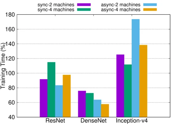
The communication overhead caused by exchange information between workers and the pa- rameter server has been known as a key factor in the runtime performance. GPUs and ASICs are getting faster and faster, while the demand for network bandwidth is growing beyond the physical network capacity. As a result, the communication overhead outweighs the benefit of parallel com- puting and becomes the bottleneck of the training process. Table 1.1 and Figure 1.1 show some training records of modern deep learning models. It’s obvious that the speedup of distributed training is highly correlated to the bits generated per second (bps) on each workers. For exam- ple, although DenseNet has more parameters than the ResNet, its bps is smaller and the training time is shorter because the model is more compute-intensive. On the other hand, the model size of Inception-v4 grows significantly larger, resulting in large communication overhead compared to computation time, and therefore, the distributed training is actually slower than on a single machine.

Model batch size # of parameters step/sec bps

ResNet 64 1.73M 13.5 746.5M

DenseNet 64 2.22M 2.92 207.2M

Inception-v4 32 42.65M 1.47 2.01G

Table 1.1: Training Records of Modern Deep Learning Models in Tensorflow.

40 60 80 100 120 140 160 180

ResNet DenseNet Inception-v4

Training Time (%)

sync-2 machines sync-4 machines

async-2 machines async-4 machines

Figure 1.1: Performance of Distributed Tensorflow.

Major optimization methods adopted for the network issue can be categorized into three types:

data placement, consistency control, and compression.

Data Placement Parameter server is an abstract concept and can be divided into multiple server nodes. In this kind of setting, the system needs to decide in which server a parameter is placed. If a suitable data placement policy is implemented, the communication latency can be reduced.

Consistency Control Accessing parameter server for updating the model incurs substantial overhead on the system. In recent works, researchers usually employ loose synchronization and create inconsistent models to decrease waiting time for network transfer. Besides, in the same syn- chronization restriction, there is room for performance improvement by fine-grained transmission control.

Compression Instead of reducing the frequency of the communication, the system can reduce the size of each message. There are mainly two research directions – quantization and sparsifica- tion. The former uses fewer bits to represent each parameter; the latter transmits only important parameters. Their goal is to achieve high compression ratio and low accuracy loss.

Existing systems and researches use ad-hoc strategies or intricate architectures to implement these optimization techniques. The main problem with existing approaches is that, when we want to employ some methods, we need to insert codes throughout the codebase. Furthermore, if mul- tiple kinds of optimizations are required, it is difficult to decouple the functions between them and analyze the performance of different optimization combinations. With these observations, we pro- pose a Modularized Parameter Server , an architecture that consists of a couple of key components that can be overridden without much effort and allows developers to easily incorporate optimiza- tion techniques in the training process. Experimental results show that the distributed training system based on our modularized parameter server efficiently supports various optimizations and achieves near-linear speedup without sacrificing much accuracy.

The main contributions of this paper are as follows.

• We propose a modularized parameter server architecture that can adopt various optimization techniques with ease.

• We implement a distributed deep learning system based on Tensorflow with the modularized parameter server, and implement a number of optimization methods in the system.

• We conduct experiments to prove the effectiveness of the proposed system and analyze the performance gain with single and multiple optimizations. The result indicates that we can improve the performance while maintaining the model accuracy by using the proposed system and combining multiple optimization techniques to reduce communication overhead.

The rest of this paper is organized as follows. Chapter 2 introduces the basics of deep learning, distributed training, and communication optimization techniques. Chapter 3 discusses the related

works. Chapter 4 describes the architecture of our modularized parameter server and our imple- mentation of distributed deep learning system based on Tensorflow. In Chapter 5, we implement different optimization techniques and conduct experiments to evaluate the system. Chapter 6 gives some concluding remarks.

Chapter 2

Background

In this chapter, we introduce deep learning by using image classification as an example. Then we describe the distributed training with and without parameter server. In the end, we summarize the optimization techniques for network communication.

2.1 Deep Learning

A deep learning model fw is a function defined by a set of trainable parameters w to ap- proximate a target function z. The model is typically composed of multiple layers, and layers are connected to form a network. For example, there might be three layers representing three functions fw⁽¹⁾1, fw⁽²⁾2 and fw⁽³⁾3 respectively. These layers constitute to form the model fw(x) = f_w⁽³⁾₃(f_w⁽²⁾₂(f_w⁽¹⁾₁(x))). Convolutional layer and fully-connected layer are two common types of para- metric functions.

Taking image classification as an example, y = z(x) means that z maps an input image x ∈ X to a true label y. X is a set of image samples constructed from D, a probability distribution of real world data. In general, we want to find a best set of parameter w^∗ to minimize the expectation of loss function `(fw(x), y), which is calculated as the difference between the predicted label f_w(x) and the true label y. The optimization problem is shown as Equation 2.1. The process to solve this problem is called Training a deep learning model.

w^∗= argmin

w

x∼DE [`(f_w(x), y)] (2.1)

The most widely used method to train a model is Stochastic Gradient Descent (SGD). SGD iteratively modifies parameters by using elements in dataset X. In each iteration, loss value is calculated first by performing a forward pass through layers. Then, a backward pass propagates the loss value back through the network to compute the gradient g with respect to the parameters, and then the gradient is applied to the parameters with a learning rate η. Figure 2.1 shows the

training process by using image classification as an examlpe.

∂loss

∂w₃

f1 : Convolutional Layer f2 : Convolutional Layer f3 : Fully Connected Layer

x

d f3

d f2

d f1 w₃

Loss Function True

Label

∂loss

∂w₂

∂loss

∂w₁

∂loss

∂x

Forward Pass Backward Pass w₂

w₂

Figure 2.1: Training a Deep Learning Model

2.2 Distributed Training

As mentioned in chapter 1, as the training data set is large, the training process usually needs to run on a distributed system. In data parallelism, gradients are computed by multiple workers and must be aggregated, so a distributed version of the SGD algorithm is required. Algorithm 1 shows the pseudocode of distributed SGD.

Algorithm 1: Distributed SGD

Data: Training data X, T iterations, learning rate η and N nodes

1 w(0) = initial value

2 for t = 0 to T − 1 do

3 for n = 1 to N in parallel do

4 x = random sample from X

5 loss_n= `(f_w(t)(x), z(x))

6 g_n= ^∂loss_∂wⁿ

7 w(t + 1) = w(t) − η ·PN n=1g_n

To exchange gradients at Line 7, the most widely used network architecture is Parameter Server, which stores parameters of a model that are shared among nodes and can be accessed via a key-value-like interface. A different approach is using decentralized network architecture for

exchanging information. Figure 2.2 shows these two communication patterns. The choice be- tween using either architecture is non-trivial and still an open problem [16]. We choose parameter server for the following reasons. (i) Centralized architecture has been proved to be a solid ap- proach by many practical deep learning frameworks, including Tensorflow [17], MXNet [18], and CNTK [19]. (ii) By keeping a global view of the training process, a parameter server provides more opportunities to decrease communication cost and maintain accuracy by performing suit- able optimizations, such as constant learning rate schedule [20] and momentum correction [21].

(iii) By relaxing synchronization restriction, parameter server can further improve the performance at scale without introducing convergence issue in the decentralized method [22].

Parameter Server

Worker

Worker Worker

Worker

(a) Centralized Architecture

Worker

Worker Worker

Worker

(b) Decentralized Architecture Figure 2.2: Communication Patterns

2.3 Communication Optimization

Although distributed learning with Algorithm 1 gets benefit from parallel computing, the in- trinsic synchronization property and the need to transmit huge volumes of data over network drag the performance down. Some previous works such as Li et al. 2014 [12] and GeePs [15] achieve great scalability by using high-end network infrastructure, for example, Infiniband and 40 Gigabit Ethernet. In this work, our goal is to enable such distributed training with commodity network infrastructure to democratize deep learning for millions of practitioners who cannot afford expen- sive equipments. Researchers have been developing many optimization techniques to solve this issue. These techniques can be categorized as follows.

2.3.1 Placement

Since the responsibility of parameter server can be divided into multiple server nodes, place- ment of each parameter becomes a critical issue. For example, GeePs [15] splits parameters into tables which composed of many fixed-size rows, and places rows into servers. Tensorflow [17]

defines parameters of the same layer as a Variable, and places variables in a round-robin way by default. It also provides another strategy that greedily places variables on the least-loaded server when each variable is processed. However, both strategies suffer from the sensitivity to the order of variable creation.

Layer-based load balancing problem can be seen as a Multi-Way Number Partitioning prob- lem [23], which is NP-complete. A simple heuristic algorithm for this problem is to sort layers in descending order and assign in turn to the server with the least load. Algorithm 2 shows the heuristic algorithm.

Algorithm 2: Heuristic Multi-Way Number Partitioning Data: A set of layers L, N nodes

Result: A set of layers for each nodes P

1 Sort L in descending order according to the sizes

2 foreach l in L do

3 n = node that has the least load

4 Add l to Pn

2.3.2 Consistency Control

In Algorithm 1, each iteration in the training process computes with the same up-to-date w on each worker. To accomplish such Bulk Synchronous Parallelism, every node has to exchange their updates before fetching new data to compute, as shown in Figure 2.3a. There are two rea- sons why bulk synchronous parallelism may incur heavy overhead on the system and harm the scalability: (1) Network Congestion occurs when the workers generate more data than the network can handle, resulting in transmission delay and waiting time that is significant relative to the com- puting time,and (2) Performance Fluctuation happens when some workers (so-called stragglers) occasionally become much slower than the others. To deal with these issues, recent works relax synchronization requirements for the distributed SGD.

Total Asynchronous Parallelism, shown in Figure 2.3b, is an asynchronous scheme that allows workers to access parameters independently. At time t, a worker may read w that only contains updates before time tc. t − tc is called staleness. Despite high efficiency of total asynchronous parallelism, it has been proved that the staleness would affect convergence of training [24].

There are other asynchronous schemes. Stale Synchronous Parallelism [25] is a middle ground

between bulk synchronous parallelism and total asynchronous parallelism, guaranteeing that miss- ing updates in each worker is enforced to be bounded by a threshold before a computation is carried on. Figure 2.3c illustrates stale synchronous parallelism and shows that the demand for network bandwith and the level of performance fluctuation can be reduced. Ho et al. [26] and Tsuzuku et al. [27] proposed adaptive communication approaches instead of the fixed period method. The adaptive approaches, shown in Figure 2.3d, send and request data only when some criteria are met. These schemes significantly reduce the communication traffic while maintaining the quality of convergence.

Parameter Server Iteration 0

Iteration 0

Iteration 1

Iteration 1 Time Node 1

Node 2 _{Sync Sync}

Straggle

(a) Bulk Synchronous Parallelism

Parameter Server Iteration 0

Iteration 0

Iteration 1

Iteration 1 Time Node 1

Node 2

t_c

Iteration 2 Access at will t

(b) Total Asynchronous Parallelism

Parameter Server Iteration 0

Iteration 0

Iteration 1

Iteration 1 Time Node 1

Node 2

Iteration 2

Iteration 2 Threshold = 1

(c) Stale Synchronous Parallelism

Parameter Server Iteration 0

Iteration 0

Iteration 1

Iteration 1 Time Node 1

Node 2

Iteration 2

Iteration 2 Iteration 3

Meet criterion

(d) Adaptive Approach

Figure 2.3: Synchronization Schemes

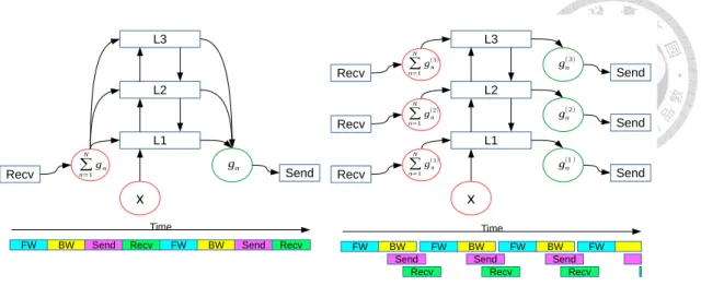
In addition to the synchronization scheme, fine-grained transmission control can improve the performance, too. For example, Poseidon [28], a scalable architecture for distributed learning, uses distributed wait-free backpropagation. In traditional backpropagation, shown in Figure 2.4a, the system receives all gradients at once, computes the forward and backward pass, and then sends full gradient at once. Distributed wait-free backpropagation, shown in Figure 2.4b, receives partial gradient and computes one layer at a time. Therefore, it can overlap the computation and data exchange to improve the communication efficiency. Furthermore, Tsai et al. [29] analyzed various computation and communication schedulings for distributed deep learning.

2.3.3 Compression

Reducing the size of each message can also relieve network congestion. One type of tech- niques is Quantization, which decreases the size of data representation for gradients or parameters.

Since values in deep learning are usually represented by IEEE 754 format, some works [30, 31, 32]

quantize values by reducing the precision or dynamic range of floating point. Another way to do quantization is to put the values into buckets. Seide et al. 2014 [33] proposed 1-bit SGD with error feedback. QSGD [34] and Terngrad [35] employ stochastic rounding. The former uses multi-level schemes to make the trade-off between compression ratio and iteration quality; the latter ternarizes

L3

L2

L1

∑

n=1 N

g_n

x

gn

Time

FW BW

Recv Send

Send Recv FW BW Send Recv

(a) Traditional Backpropagation

L3

L2

L1

x

Time

FW BW

Recv Send

Send Recv Recv

Recv

Send Send

FW BW

Send Recv

FW BW

Send Recv

FW

∑n=1 N

g(1)n

∑n=1 N

gn(2)

∑n=1 N

gn(3)

g_n^{(1 )} g_n⁽²⁾ g_n⁽³⁾

(b) Distributed Wait-free Backpropagation

Figure 2.4: An Example of Transmission Control

and clips the gradient to achieve high compression ratio without sacrificing much accuracy.

Because each of updates is of different importance in an iteration, Sparsification, which only sends significant gradients, can be used. Storm 2015 [36] proposed the first system that uses sparsification with a static threshold to determine which values can be transmitted and keeps a residual bufferto store values which are not sent. Other works [37, 21] proposed relative threshold, such as top 1 %, based on the absolute values of the gradient.

Chapter 3

Related Work

Researchers have developed many parameter servers with different optimization techniques.

This chapter supplements these works which are related to topics discussed in this paper.

Tensorflow [17] is a popular deep learning framework and has built-in parameter server con- figurations. MXNet [18] and CNTK [19] are two other frameworks. Both of them also have parameter server as components, named PS-Lite [38] and Multiverso [39] respectively. These frameworks provide simple interfaces for distributed training with bulk synchronous parallelism and total asynchronous parallelism.

Iterstore [40] is a parameter server that exploits repeating patterns in machine learning appli- cations and uses these patterns to apply some optimizations, including data caching, informing prefetch, and partitioning decisions. Its follow-up study, GeePs [15], is a GPU-specialized param- eter server which uses repeating patterns to improve CPU-GPU memory management.

Bosen [41] is another parameter server system that aims to maximize the network communica- tion efficiency by using stale synchronous parallelism and managed communication. The managed communication models the network as a leaky bucket and prioritizes parameters to be sent.

There are many other systems that use parameter server: Poject Adam [13] reduces the amount of information transmitted over the network by sending loss and the output of previous layer at fully-connected layer; Gaia [42] designs a hierarchical parameter server infrastructure for a geo- distributed system and only synchronizes important updates; Angel [20] uses a constant learning rate schedule to suppress the harm of stragglers. To the best of our knowledge, this paper is the first work to propose a modularized parameter server as a platform for network optimization research and practical system development. With this platform, we can analyze different combinations of optimization techniques and develop new compression or transmission algorithms.

Chapter 4

Architecture

In this chapter, we introduce modularized parameter server, where those optimizations can be easily applied. Then an implementation of a distributed training system based on modularized parameter server and Tensorflow is described.

4.1 Modularized Parameter Server

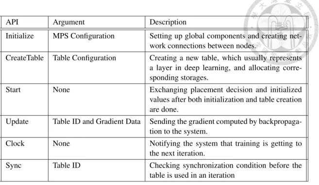
Modularized parameter server is a C++ library which provides a set of APIs similar to prior parameter servers. To be a flexible infrastructure, common functions of various communication optimization techniques in the training process are packed into C++ classes that can be modified or inherited without much effort. Figure 4.1 and Table 4.1 show the overview of the architecture and the summary of APIs respectively. In the folloing paragraphs, we introduce the detail of each component.

Each Table in the parameter server represents a layer in deep learning. A Client Table main- tains memory storage and buffers in a worker; a Server Table maintains table partitions assigned to a server node. Both types of table maintain some metadata, such as the size and value type of table.

A Storage manages the data structure where parameters or gradients are stored and implements behaviors of assigning, updating, encoding, and decoding. There are five types of storage in a ta- ble: (i) Gradient Storage represents a gradient computed from the deep learning framework and sends the gradient to the transmit buffer. (ii) Transmit Buffer stores gradients that have not been sent and encodes the content by optimization techniques such as compression and partition split when the gradients are about to be sent over the network. (iii) Server Storage decodes data sent from workers and aggregates gradients by various gradient descent algorithms [43]. Like trans- mit buffer, server storage supports implementation of a server-side encoding scheme. (iv) Apply Bufferdecodes data received from servers and keeps the content until updates are applied to the framework’s working memory. (v) Worker Storage manages device memory of the deep learning

API Argument Description

Initialize MPS Configuration Setting up global components and creating net- work connections between nodes.

CreateTable Table Configuration Creating a new table, which usually represents a layer in deep learning, and allocating corre- sponding storages.

Start None Exchanging placement decision and initialized

values after both initialization and table creation are done.

Update Table ID and Gradient Data Sending the gradient computed by backpropaga- tion to the system.

Clock None Notifying the system that training is getting to the next iteration.

Sync Table ID Checking synchronization condition before the table is used in an iteration

Table 4.1: APIs of Modularized Parameter Server

Deep Learning Framework Worker

Storage

Gradient Storage

Comm

Transmit Buffer Placement

Manager

Server Storage Apply

Buffer

Consistency Controller

update update

encode

decode encode

decode

Worker Server

Consistency Controller

trigger

trigger request request

Figure 4.1: Modularized Parameter Server

framework. It also implements the behavior of updating data into memory. For example, if the worker receives aggregated gradient, the gradient is added to parameters in the memory. In other cases, if the worker receives up-to-date parameters, the memory can be directly overwritten by the new parameter values.

Placement Manager uses a decision function to divide tables into partitions if needed and assign these partitions to server nodes according to placement strategy. When transmit buffer needs to encode data or consistency controller wants to make a request, placement manager passes the partition information to them.

Consistency Controllerdecides when and which data is sent or applied. The main responsi- bilities include sending gradients from transmit buffer to server storage, sending data from server storage to apply buffer, applying data in apply buffer to worker storage, and ensuring all the con- sistency requirements are met. It can also actively request pieces of data from other nodes if the scheme demands. There are many call sites of the controller, such as update, sync, clock, and data or request receiving.

Finally, Comm is a non-overridable component. It provides primitive interfaces for network communication, e.g., global barrier and client/server-side push/pull. In our implementation, we use gRPC [44] as the intermidiate communication mechanism to fairly compare the performance between Tensorflow and our system.

4.2 Use Case

Here we use an example to show how modularized parameter server can help developers imple- ment optimization techniques. In this case, we want to develop a training system with round-robin placement policy, top-1% sparsification, and stale synchronous parallelism.

First, we inherit the placement class and implement the round-robin policy in decision function by assigning partitions to servers in turn, as Code 4.1 shows. The behaviors of encoding and decoding in storages need to be customized to adopt the top-1% sparsification. Code 4.2 shows the encoding function in transmit buffer that partially sorts data to get top 1% gradient values and encodes them into a per server byte stream which contains index/value pairs. Then server storage in Code 4.3 decodes the received byte stream and applies to data storage. Server storage and apply buffer also have similar encoding/decoding procedure. Finally, stale synchronous parallelism is impelemeted in consistency controller, shown in Code 4.4. It ensures that the synchronization requirements are met before the client uses the layer, pushes and pulls data when needed, checks the staleness before sending data from server, and notifies the client and server when requirements are fulfilled.

Code 4.1: Round-robin Placement

class RoundRobinPlacement: public Placement {

public:

void Decision() override { int last = 0;

for (auto&& config: Lib::TableConfigs()) { table_to_partitions_[config.id][last] =

Partition{0, config.size};

last = (last + 1) % Lib::NumHosts();

} } };

Code 4.2: Transmit Buffer with Top-1% Sparsification template<typename T>

class TfTransmitBuffer: public DenseStorage<T>

{

public:

map<Hostid, Bytes> Encode(

const Partitions& partitions) override { vector<int> indexes(this->data_.size());

iota(indexes.begin(), indexes.end(), 0);

auto middle = partial_sort_top_precentage(

indexes, COMPRESSION_RATIO);

auto part = partitions.begin();

map<Hostid, Bytes> ret;

for (auto it = indexes.begin();

it != middle; ++it) { int idx = *it;

while (idx >= part->second.end) ++part;

Hostid server = part->first;

T& val = this->data_[idx];

append(ret, idx, val);

val = 0;

}

return ret;

} };

Code 4.3: Server Storage with Top-1% Sparsification template<typename T>

class TfServerStorage: public DenseStorage<T>

{

public:

Bytes Encode() override {

// ... similar to transmit buffer ...

}

void Decode(Hostid from, Hostid to, const Bytes& bytes) override { if (from == to) return;

auto it = bytes.begin();

while (it != bytes.end()) { auto [next, idx, val] =

decode_element(it);

this->data_[idx] += val;

it = next;

} } };

Code 4.4: Stale Synchronous Parallelism class SSPConsistency: public Consistency

{

public:

void ClientSync(Tableid id,

Iteration iteration) override { auto&& table = get_table(id);

std::unique_lock<std::mutex> lock(table.mu);

table.cv.wait(lock,

[this, &table, iteration]{

Iteration min = min_partition(

table.iterations.begin(), table.iterations.end());

return min >= iteration - staleness_ - 1;

});

}

void AfterClientUpdate(Tableid id, const Storage& storage,

Iteration iteration) override { auto&& table = get_table(id);

Iteration min = min_partition(

table.iterations.begin(), table.iterations.end());

if (min < iteration - staleness_) { push_to_server();

pull_from_server();

} }

void BeforeGetServerData(

Hostid client, Tableid id, Iteration iteration) override { auto&& table = get_table(id);

std::unique_lock<std::mutex> lock(table.server_mu);

table.server_cv.wait(lock, [this, &table, iteration]{

Iteration min = min_parition(

table.server_iterations.begin(), table.server_iterations.end());

return min >= iteration - staleness_;

});

}

void AfterClientPushHandler(Hostid client, Tableid id, Iteration iteration,

const Bytes& bytes) override { auto&& table = get_table(id);

Iteration min = min_partition(

table.server_iterations.begin(), table.server_iterations.end());

if (min >= iteration - staleness_) { table.server_cv.notify_all();

} }

void AfterServerPushHandler(Hostid server, Tableid id, Iteration iteration,

const Bytes& bytes,

Iteration iteration_now) override { auto&& table = get_table(id);

table.cv.notify_all();

}

private:

// ... some data and auxiliary functions...

};

Each component is decoupled from the main program and other components, so we can mod- ify/implement an optimization without digging into codebase or affecting other optimizations.

For example, we can replace the round-robin placement with heuristic approach mentioned in chapter 2 by a new decision function. We can also apply quantization methods in encoding and decoding function or use the adaptive synchronization method by checking the criteria at some call sites of consistency controller.

4.3 Distributed Training System

In order to compare with an existing distributed training framework, we implement a system in this work by using Tensorflow [17] as the deep learning framework mentioned in Figure 4.1. Ten- sorflow takes computation as a directed Graph. Each node in a graph represents the instantiation of an Operation, which describes an abstract computation, such as addition or matrix multiplication, and has inputs/outputs called Tensors. User programs interact with Tensorflow by using a Session.

The session can augment the currently managed graph and supports an interface named Run, which executes required computations to get outputs of specific nodes. In distributed Tensorflow, nodes are mapped onto a set of devices, and cross-device edges are replaced by a pair of send/receive nodes for cross-device communication. With this mechanism, original Tensorflow can implement different distributed training configurations including parameter server architecture.

To use modularized parameter server, the system launches an instance of modified Tensorflow per node, and each of them links to the library. There are two kinds of operations in Tensorflow that are most related to our work. Variable Op is a special stateful operation that maintains persis-

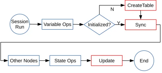
tent states across iterations. Layers in deep learning are usually represented by trainable variables, and each variable manages a tensor to store values. Another kind of operations is State Ops, which takes references of variables as inputs and can modify the underlying tensors. A subset of state ops called training ops is responsible for updating variables according to some optimization algo- rithms. We modify variable op to check whether the variable is initialized. If not, a corresponding table with related information, including size, data type, and storage types, is created first in the pa- rameter server. Then we check the synchronization condition before passing the variable to other operations. We also create a new type of operation for updating data in the parameter server and insert an updating operation after each training op node. Figure 4.2 shows the schematic flowchart of a session run.

Session

Run Variable Ops Initialized? Sync

CreateTable

Y

Other Nodes State Ops Update End

N

Figure 4.2: Parameter Server in TensorFlow

In addition to modifying Tensorflow, we also expose necessary APIs to Tensorflow’s Python bindings. At the beginning of user programs, the initialization of parameter server is called with a user-provided configuration, and the paramter server is started after the creation and initialization of variables are done. An iteration of deep learning usually includes a session run. The user needs to calls the clock function at the end of each iteration. Code 4.5 shows an example of user program.

Code 4.5: An example of user program import tensorflow as tf

tf.ps_initialize_from_file("config.pbtext")

# ... graph definition...

sess = tf.Session() sess.run(init) tf.ps_start()

for i in range(MAX_ITERATION):

sess.run(train) tf.ps_clock()

# ... evaluation ...

Chapter 5

Evaluation

In this chapter, we analyze the performance gain from different optimization techniques and evaluate the scalability of our distributed training system by training three deep learning models for image classification – GoogLeNet [4], ResNet [5], and Inception-v4 [6]. GoogLeNet, developed by Google, uses a deep learning architecture called inception to increase the depth and width of the network and wins 2014 ImageNet Large Scale Visual Recognition Competition (ILSVRC).

ResNet, developed by Microsoft, proposes residual learning to cope with the difficulty of training a very deep neural network and wins 2015 ILSVRC. Inception-v4 presents several new architectures and combines the idea of residual learning to train the model efficiently.

Two datasets are used in this evaluation. CIFAR10 [45], used by ResNet, has 60,000 32x32 images in 10 classes, with 6,000 images per class. 50,000 images are used as training images, and the other 10,000 images are used for validation. ILSVRC-2012, used by GoogLeNet and Inception-v4, consists of 1.2 million images that are categorized into 1000 classes, and a subset with 50,000 images is selected as the validation set.

Our experiment environment consists of a commodity GPU cluster which has four machines.

Each machine is equipped with a Nvidia GeForce GTX 1080 Graphics Card, a 3.70 GHz 4 cores Intel CPU, and 64 GB of RAM. The machines are connected via a 1 Gbps Ethernet interface.

Tensorflow 1.4.0 is used to develop our system and runs in parameter server configuration as the baseline. We train the model by canonical SGD with learning rate 0.1 and 20,000 iterations on each node. The performance metric is the speedup of the optimizations, measured as iteration per second ratio of distributed training against single machine training.

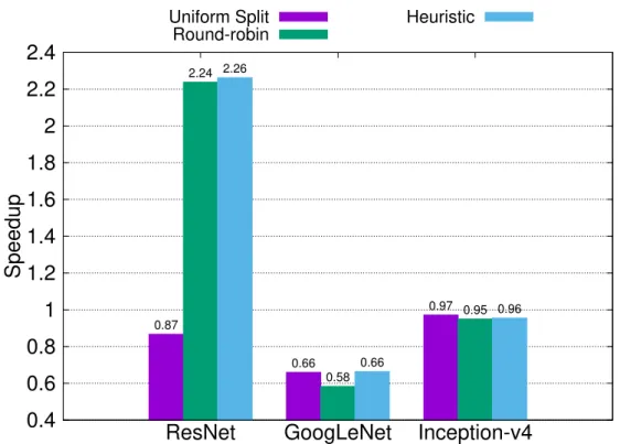
In the first set of experiment, we test three different placement strategies. Uniform Split is a parameter-based placement method that evenly splits each layer onto all of the servers. Round- robin, the default strategy in Tensorflow, places layers to each server in turn. Heuristic Method described in Algorithm 2 is implemeted, too. Figure 5.1 shows the speedup of these three place- ment strategies in different models. We observe that each strategy has different performance in different models. The main reason is that each model has different layer size distribution as shown

in Figure 5.2, and different variation of the size on each server caused by the placement strategy as shown in Figure 5.3. Despite no variation, uniform split may incur substantial increase in net- work traffic if the model has many small layers. Taking ResNet as an example, the number of partitions produced by uniform split is four times that of the number of layers, and many parti- tions are even smaller in size than the message headers and metadata. The network utilization for useful content is very low, so the performance drops significantly. However, if a model, like Inception-v4, has many large layers, standard deviations of other strategies become large. In this case, uniform split achieves the best performance among the three strategies by reducing variation.

Layer-based methods avoid the problem mentioned above, but load balance of round-robin suffers from high coefficient of variation due to the sensitivity to the order of variable creation, especially in GoogLeNet. Heuristic method effectively reduces the coefficient of variation, achieving the best and the most stable performance on average. In the following experiments, we use heuristic method as the placement strategy.

0.4 0.6 0.8 1 1.2 1.4 1.6 1.8 2 2.2 2.4

ResNet GoogLeNet Inception-v4

Speedup

Uniform Split

0.87

0.66

0.97

Round-robin

2.24

0.58

0.95

Heuristic

2.26

0.66

0.96

Figure 5.1: Speedup of Placement Strategies

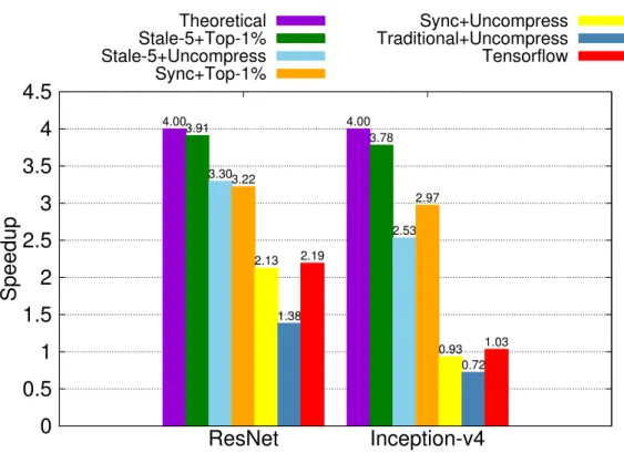
Figure 5.4 illustrates the speedup for various combinations of consistency control and com- pression scheme. We can get many properties of optimization techniques by analyzing these ex- perimental results. First, comparing traditional backpropagation (dark blue bar) with synchronous Distributed Wait-free Backpropagation(yellow bar), we found that transmission control can have big impact. ResNet and Inception-v4 achieve 1.54x and 1.29x acceleration, respectively. We also show that our architecture does not introduce too much overhead by comparing the original distributed Tensorflow (red bar) with the yellow bar. Compression by top-1% sparsification (or-

0 10 20 30 40 50 60 70 80

11 64 160 288 512

3072 819212800245763686455296768001024001351682129922949123732484608006881281537536

Count

Size

ResNet GoogLenet Inception-v4

Figure 5.2: Layer Size Distribution of Models

0 20 40 60 80 100

ResNet GooLeNet Inception-v4

0 0.5 1 1.5 2 2.5

Coefficient of variation (%) Standard Deviation (MB)

Uniform Split x

0.00 0.00 0.00

0.00 0.00 0.00

Round-robin o

16.65

61.93

22.78

0.07

1.08

2.01

Heuristic +

2.71

18.87

5.77

0.01

0.40

0.62

Figure 5.3: Variation of Placement Strategies

ange bar) and relaxing synchronization by stale synchronous parallelism with threshold 5 (blue bar) improve the performance significantly, too. For ResNet, the consistency control achieves higher speedup than compression. On the other hand, for Inception-v4, which is much bigger than ResNet, we can get more performance gain from compression. This again shows that different models with unique characteristics (such as size or layer distribution) may benefit from different optimization methods and hyper-parameters settings. Then, we combine all above optimizations (green bar) and achieve a near-theoretical speedup, 3.91x for ResNet and 3.78x for Inception-v4.

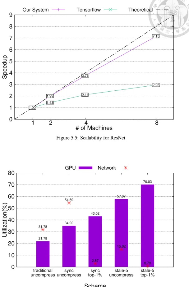
In Figure 5.5, we also show that our system is much closer to the theoretical performance than the original Tensorflow, achieving near-linear scalability.

0 0.5 1 1.5 2 2.5 3 3.5 4 4.5

ResNet Inception-v4

Speedup

Theoretical

4.00 4.00

Stale-5+Top-1%

3.91 3.78

Stale-5+Uncompress

3.30

2.53

Sync+Top-1%

3.22

2.97

Sync+Uncompress

2.13

0.93

Traditional+Uncompress

1.38

0.72

Tensorflow

2.19

1.03

Figure 5.4: Speedup for Different Optimizations

Next, we take ResNet as an example to study the changes of system resource usage caused by different optimization techniques. By analyzing GPU and network utilization shown in Figure 5.6, we can get some clues to improve the performance. The most important issue for speedup is increasing GPU utilization and decreasing the waiting time for network transfer. Distributed wait- free backpropagation overlaps the computation and transmission, raising network utilization and GPU utilization. Both compression and synchronization scheme reduce demands for network bandwidth, thereby decreasing the network utilization and increasing GPU utilization. The reason why synchronization scheme can achieve better GPU utilization and higher network utilization at the same time is that it reduces performance fluctuations by mitigating the impact of stragglers and also reducing the amount of transmission. Combining these methods further reduce network usage and the impact of performance fluctuations, resulting in increased GPU utilization.

0 1 2 3 4 5 6 7 8 9

1 2 4 8

Speedup

# of Machines

Our System Tensorflow Theoretical

1.00 1.00

1.43 1.43

2.11 2.11

2.95 2.95

1.00 1.00

1.99 1.99

3.76 3.76

7.15 7.15

Figure 5.5: Scalability for ResNet

0 10 20 30 40 50 60 70 80

traditional

uncompress sync

uncompress sync

top-1% stale-5

uncompress stale-5 top-1%

Utilization(%)

Scheme

GPU

21.78

34.92

43.02

57.67

70.03

Network

31.78

54.59

2.87

15.02

0.79

Figure 5.6: GPU and Network Utilization of ResNet

0.1 0.2 0.3 0.4 0.5 0.6 0.7 0.8 0.9

0

2000 4000 6000 8000 10000 12000 14000 16000 18000 20000

Accuracy

Iteration

Tensorflow Top-1% Stale-5

Figure 5.7: Convergence Quality of Iterations

0.1 0.2 0.3 0.4 0.5 0.6 0.7 0.8 0.9

0 500 1000 1500 2000 2500 3000

Accuracy

Elasped time(second)

Tensorflow Single Our System

Figure 5.8: Training Time to Accuracy of ResNet

Convergence time to a specific accuracy is affected by both the processing speed (iteration per second) and the convergence rate of each iteration. Figure 5.7 shows that staleness in asyn- chronous parallelism and information loss in compression do incur accuracy loss. That is, for the same number of iterations Tensorflow does have slightly higher accuracy than our method. How- ever, the processing speed of our method is much faster than Tensorflow, so that despite the slower converge due to staleness and compression, we can still achieve the same accuracy within 43%

of the training time of the original Tensorflow. For example, Figure 5.8 suggests that our method trains ResNet much faster than Tensorflow to a specific accurate. This indicates that the benefit of network optimizations, which reduces the communication time, outweighs the extra computing time required to remedy the quality loss introduced by these optimizations.

Chapter 6

Conclusion

In this paper, we summarize various communication optimizations for deep learning and pro- pose a modularized parameter server to adopt these techniques. Instead of using ad-hoc ap- proaches, our architecture uses overridable decoupling components to implement the functions required by optimizations. By doing so, we can apply most of the optimization techniques easily, examine different combinations, and analyze the performance.

We evaluate the proposed architecture by implementing a distributed training system based on Tensorflow and training three popular deep learning models – ResNet, GoogLeNet, and Inception- v4. The experimental results demonstrate that our system can get near-linear speedup for comput- ing and achieve convergent accuracy while reducing the communication overhead. This reduces half of training time for ResNet than the original Tensorflow. The experiments also show that dif- ferent models may benefit from different optimization techniques and hyper-parameters settings.

This is because characteristics of models, such as size, computation or layer distribution, affect properties of transmission and effects of optimizations.

Looking into the performance gain, we can get some clues for enhancements. Both com- pression and asynchronous communication reduce the amount of transmitted data to ease network congestion, and the later also mitigates performance fluctuations. The quality loss of iterations can be reduced by better compression algorithms that decrease the information loss without sacrificing the compreassion ratio, and by better transmission control that uses network bandwidth effectively to decrease the staleness without violating the synchronization requirements. With these investi- gations, we plan to research and develop new optimization techniques to further improve our system.

Bibliography

[1] Alex Krizhevsky, Ilya Sutskever, and Geoffrey E. Hinton. Imagenet classification with deep convolutional neural networks. In Proceedings of the 25th International Conference on Neu- ral Information Processing Systems - Volume 1, NIPS’12, pages 1097–1105, USA, 2012.

Curran Associates Inc.

[2] Olga Russakovsky, Jia Deng, Hao Su, Jonathan Krause, Sanjeev Satheesh, Sean Ma, Zhi- heng Huang, Andrej Karpathy, Aditya Khosla, Michael Bernstein, Alexander C. Berg, and Li Fei-Fei. ImageNet Large Scale Visual Recognition Challenge. International Journal of Computer Vision (IJCV), 115(3):211–252, 2015.

[3] Karen Simonyan and Andrew Zisserman. Very deep convolutional networks for large-scale image recognition. CoRR, abs/1409.1556, 2014.

[4] Christian Szegedy, Wei Liu, Yangqing Jia, Pierre Sermanet, Scott E. Reed, Dragomir Anguelov, Dumitru Erhan, Vincent Vanhoucke, and Andrew Rabinovich. Going deeper with convolutions. CoRR, abs/1409.4842, 2014.

[5] Kaiming He, Xiangyu Zhang, Shaoqing Ren, and Jian Sun. Deep residual learning for image recognition. CoRR, abs/1512.03385, 2015.

[6] Christian Szegedy, Sergey Ioffe, and Vincent Vanhoucke. Inception-v4, inception-resnet and the impact of residual connections on learning. CoRR, abs/1602.07261, 2016.

[7] Gao Huang, Zhuang Liu, and Kilian Q. Weinberger. Densely connected convolutional net- works. CoRR, abs/1608.06993, 2016.

[8] Dario Amodei, Rishita Anubhai, Eric Battenberg, Carl Case, Jared Casper, Bryan Catan- zaro, Jingdong Chen, Mike Chrzanowski, Adam Coates, Greg Diamos, Erich Elsen, Jesse Engel, Linxi Fan, Christopher Fougner, Tony Han, Awni Y. Hannun, Billy Jun, Patrick LeGresley, Libby Lin, Sharan Narang, Andrew Y. Ng, Sherjil Ozair, Ryan Prenger, Jonathan Raiman, Sanjeev Satheesh, David Seetapun, Shubho Sengupta, Yi Wang, Zhiqian Wang, Chong Wang, Bo Xiao, Dani Yogatama, Jun Zhan, and Zhenyao Zhu. Deep speech 2: End- to-end speech recognition in english and mandarin. CoRR, abs/1512.02595, 2015.

[9] Minh-Thang Luong, Hieu Pham, and Christopher D. Manning. Effective approaches to attention-based neural machine translation. CoRR, abs/1508.04025, 2015.

[10] Sergey Levine, Chelsea Finn, Trevor Darrell, and Pieter Abbeel. End-to-end training of deep visuomotor policies. CoRR, abs/1504.00702, 2015.

[11] Leon A. Gatys, Alexander S. Ecker, and Matthias Bethge. A neural algorithm of artistic style. CoRR, abs/1508.06576, 2015.

[12] Mu Li, David G. Andersen, Jun Woo Park, Alexander J. Smola, Amr Ahmed, Vanja Josi- fovski, James Long, Eugene J. Shekita, and Bor-Yiing Su. Scaling distributed machine learning with the parameter server. In Proceedings of the 11th USENIX Conference on Op- erating Systems Design and Implementation, OSDI’14, pages 583–598, Berkeley, CA, USA, 2014. USENIX Association.

[13] Trishul Chilimbi, Yutaka Suzue, Johnson Apacible, and Karthik Kalyanaraman. Project adam: Building an efficient and scalable deep learning training system. In Proceedings of the 11th USENIX Conference on Operating Systems Design and Implementation, OSDI’14, pages 571–582, Berkeley, CA, USA, 2014. USENIX Association.

[14] Eric P. Xing, Qirong Ho, Wei Dai, Jin-Kyu Kim, Jinliang Wei, Seunghak Lee, Xun Zheng, Pengtao Xie, Abhimanu Kumar, and Yaoliang Yu. Petuum: A new platform for distributed machine learning on big data. In Proceedings of the 21th ACM SIGKDD International Con- ference on Knowledge Discovery and Data Mining, KDD ’15, pages 1335–1344, New York, NY, USA, 2015. ACM.

[15] Henggang Cui, Hao Zhang, Gregory R. Ganger, Phillip B. Gibbons, and Eric P. Xing. Geeps:

Scalable deep learning on distributed gpus with a gpu-specialized parameter server. In Pro- ceedings of the Eleventh European Conference on Computer Systems, EuroSys ’16, pages 4:1–4:16, New York, NY, USA, 2016. ACM.

[16] Xiangru Lian, Ce Zhang, Huan Zhang, Cho-Jui Hsieh, Wei Zhang, and Ji Liu. Can decentral- ized algorithms outperform centralized algorithms? a case study for decentralized parallel stochastic gradient descent. In I. Guyon, U. V. Luxburg, S. Bengio, H. Wallach, R. Fer- gus, S. Vishwanathan, and R. Garnett, editors, Advances in Neural Information Processing Systems 30, pages 5330–5340. Curran Associates, Inc., 2017.

[17] Martin Abadi, Paul Barham, Jianmin Chen, Zhifeng Chen, Andy Davis, Jeffrey Dean, Matthieu Devin, Sanjay Ghemawat, Geoffrey Irving, Michael Isard, Manjunath Kudlur, Josh Levenberg, Rajat Monga, Sherry Moore, Derek G. Murray, Benoit Steiner, Paul Tucker, Vi- jay Vasudevan, Pete Warden, Martin Wicke, Yuan Yu, and Xiaoqiang Zheng. Tensorflow: A

system for large-scale machine learning. In 12th USENIX Symposium on Operating Systems Design and Implementation (OSDI 16), pages 265–283, 2016.

[18] Tianqi Chen, Mu Li, Yutian Li, Min Lin, Naiyan Wang, Minjie Wang, Tianjun Xiao, Bing Xu, Chiyuan Zhang, and Zheng Zhang. Mxnet: A flexible and efficient machine learning library for heterogeneous distributed systems. CoRR, abs/1512.01274, 2015.

[19] Frank Seide and Amit Agarwal. Cntk: Microsoft’s open-source deep-learning toolkit. In Proceedings of the 22Nd ACM SIGKDD International Conference on Knowledge Discovery and Data Mining, KDD ’16, pages 2135–2135, New York, NY, USA, 2016. ACM.

[20] Jiawei Jiang, Bin Cui, Ce Zhang, and Lele Yu. Heterogeneity-aware distributed parameter servers. In Proceedings of the 2017 ACM International Conference on Management of Data, SIGMOD ’17, pages 463–478, New York, NY, USA, 2017. ACM.

[21] Yujun Lin, Song Han, Huizi Mao, Yu Wang, and William Dally. Deep gradient compression:

Reducing the communication bandwidth for distributed training. 2018.

[22] Peter H. Jin, Qiaochu Yuan, Forrest N. Iandola, and Kurt Keutzer. How to scale distributed deep learning? 2016.

[23] Richard E. Korf. Multi-way number partitioning. In Proceedings of the 21st International Jont Conference on Artifical Intelligence, IJCAI’09, pages 538–543, San Francisco, CA, USA, 2009. Morgan Kaufmann Publishers Inc.

[24] Feng Niu, Benjamin Recht, Christopher Re, and Stephen J. Wright. Hogwild!: A lock- free approach to parallelizing stochastic gradient descent. In Proceedings of the 24th Inter- national Conference on Neural Information Processing Systems, NIPS’11, pages 693–701, USA, 2011. Curran Associates Inc.

[25] Qirong Ho, James Cipar, Henggang Cui, Jin Kyu Kim, Seunghak Lee, Phillip B. Gibbons, Garth A. Gibson, Gregory R. Ganger, and Eric P. Xing. More effective distributed ml via a stale synchronous parallel parameter server. In Proceedings of the 26th International Con- ference on Neural Information Processing Systems - Volume 1, NIPS’13, pages 1223–1231, USA, 2013. Curran Associates Inc.

[26] Jan-Jan Wu Li-Yung Ho and Pangfeng Liu. Adaptive communication for distributed deep learning on commodity gpu cluster. In 2018 18th IEEE/ACM International Symposium on Cluster, Cloud and Grid Computing (CCGrid 2018), CCGRID’18, 2018.

[27] Yusuke Tsuzuku, Hiroto Imachi, and Takuya Akiba. Variance-based gradient compression for efficient distributed deep learning. CoRR, abs/1802.06058, 2018.

[28] Hao Zhang, Zeyu Zheng, Shizhen Xu, Wei Dai, Qirong Ho, Xiaodan Liang, Zhiting Hu, Jin- liang Wei, Pengtao Xie, and Eric P. Xing. Poseidon: An efficient communication architecture for distributed deep learning on gpu clusters. In Proceedings of the 2017 USENIX Confer- ence on Usenix Annual Technical Conference, USENIX ATC ’17, pages 181–193, Berkeley, CA, USA, 2017. USENIX Association.

[29] Pangfeng Liu Ching-Yuan Tsai, Ching-Chi Lin and Jan-Jan Wu. Computation and commu- nication scheduling optimization for distributed deep learning systems.

[30] Suyog Gupta, Ankur Agrawal, Kailash Gopalakrishnan, and Pritish Narayanan. Deep learn- ing with limited numerical precision. In Proceedings of the 32Nd International Conference on International Conference on Machine Learning - Volume 37, ICML’15, pages 1737–1746.

JMLR.org, 2015.

[31] Tim Dettmers. 8-bit approximations for parallelism in deep learning. CoRR, abs/1511.04561, 2015.

[32] Urs K¨oster, Tristan Webb, Xin Wang, Marcel Nassar, Arjun K Bansal, William Constable, Oguz Elibol, Scott Gray, Stewart Hall, Luke Hornof, Amir Khosrowshahi, Carey Kloss, Ruby J Pai, and Naveen Rao. Flexpoint: An adaptive numerical format for efficient training of deep neural networks. In I. Guyon, U. V. Luxburg, S. Bengio, H. Wallach, R. Fergus, S. Vishwanathan, and R. Garnett, editors, Advances in Neural Information Processing Sys- tems 30, pages 1742–1752. Curran Associates, Inc., 2017.

[33] Frank Seide, Hao Fu, Jasha Droppo, Gang Li, and Dong Yu. 1-bit stochastic gradient descent and application to data-parallel distributed training of speech dnns. In Interspeech 2014, September 2014.

[34] Dan Alistarh, Demjan Grubic, Jerry Li, Ryota Tomioka, and Milan Vojnovic. Qsgd:

Communication-efficient sgd via gradient quantization and encoding. In I. Guyon, U. V.

Luxburg, S. Bengio, H. Wallach, R. Fergus, S. Vishwanathan, and R. Garnett, editors, Ad- vances in Neural Information Processing Systems 30, pages 1709–1720. Curran Associates, Inc., 2017.

[35] Wei Wen, Cong Xu, Feng Yan, Chunpeng Wu, Yandan Wang, Yiran Chen, and Hai Li. Tern- grad: Ternary gradients to reduce communication in distributed deep learning. In I. Guyon, U. V. Luxburg, S. Bengio, H. Wallach, R. Fergus, S. Vishwanathan, and R. Garnett, editors, Advances in Neural Information Processing Systems 30, pages 1509–1519. Curran Asso- ciates, Inc., 2017.

[36] Nikko Strom. Scalable distributed DNN training using commodity GPU cloud computing. In

INTERSPEECH 2015, 16th Annual Conference of the International Speech Communication Association, Dresden, Germany, September 6-10, 2015, pages 1488–1492, 2015.

[37] Alham Fikri Aji and Kenneth Heafield. Sparse communication for distributed gradient de- scent. In Proceedings of the Conference on Empirical Methods in Natural Language Pro- cessing, Copenhagen, Denmark, September 2017.

[38] dmlc. Ps-lite. https://github.com/dmlc/ps-lite, 2015.

[39] Microsoft. Multiverso. https://github.com/Microsoft/Multiverso, 2016.

[40] Henggang Cui, Alexey Tumanov, Jinliang Wei, Lianghong Xu, Wei Dai, Jesse Haber- Kucharsky, Qirong Ho, Gregory R. Ganger, Phillip B. Gibbons, Garth A. Gibson, and Eric P.

Xing. Exploiting iterative-ness for parallel ml computations. In Proceedings of the ACM Symposium on Cloud Computing, SOCC ’14, pages 5:1–5:14, New York, NY, USA, 2014.

ACM.

[41] Jinliang Wei, Wei Dai, Aurick Qiao, Qirong Ho, Henggang Cui, Gregory R. Ganger, Phillip B. Gibbons, Garth A. Gibson, and Eric P. Xing. Managed communication and consis- tency for fast data-parallel iterative analytics. In Proceedings of the Sixth ACM Symposium on Cloud Computing, SoCC ’15, pages 381–394, New York, NY, USA, 2015. ACM.

[42] Kevin Hsieh, Aaron Harlap, Nandita Vijaykumar, Dimitris Konomis, Gregory R. Ganger, Phillip B. Gibbons, and Onur Mutlu. Gaia: Geo-distributed machine learning approaching LAN speeds. In 14th USENIX Symposium on Networked Systems Design and Implementation (NSDI 17), pages 629–647, Boston, MA, 2017. USENIX Association.

[43] Sebastian Ruder. An overview of gradient descent optimization algorithms. CoRR, abs/1609.04747, 2016.

[44] Google. grpc. https://grpc.io.

[45] Alex Krizhevsky, Vinod Nair, and Geoffrey Hinton. Cifar-10, 2009.