Some improvements on the procedure of modeling and analysis for space-time ARMA models
對於時空
ARMA 序列分析及建模程序的一些改進
Cheng-Yu Lee Asia University [email protected]
Abstract
Correlation in space and in time is a common phenomenon among biological and environmental processes. However, in space-time ARMA modeling which is a widely used modeling for space-time correlated process, there exist some difficulties in the modeling procedure, that have impeded practical applications since the statistical theory was developed.
The difficulties include no robust optimization algorithm and no appropriate criteria for space-time model evaluation. In this paper, a space-time extension of Hannan-Rissanen algorithm is suggested for accelerating the modeling process and improving robustness while optimizing model parameters. This study makes the space-time modeling practical.
Keywords:space-time autoregressive moving average model; STARMA; Hannan-Rissanen Algorithm;
Introduction
Biological and environmental data are often organized by units of time as well as by geographic locations[4]. The processes that produce such data may have strong correlations not only in time but also in space. With increasing accessibility and accuracy in remote sensing technology, large scale analyses and data collection (especially in space) of space-time data become possible. This trend highlights the importance and necessity of space-time analysis in various disciplines.
The processes in these systems are dynamically (and often systemically) self- or inter-correlated in space and in time. Analyses considering only time or
only space may produce misleading results and be unable to reveal the dynamical behavior of the system.
In fact, biological or environmental processes such as epidemics, succession, competition, evolution, interactions, pollutant spreading, and population dynamics, assume that the elements of such a system close to one another in space or in time are more likely to be affected by the same generating process.
The lack of spatio-temporally explicit analytical framework is considered to be a major obstacle to understanding the fundamental mechanisms of such processes.
Spatio-temporal models have gained widespread popularity for the last decade. One major reason for this is an abundance of new challenging applications arising in the environmental sciences and epidemiology. Typical examples include forecasting of global climate change, infectious disease mapping[11], and their inter-relationship[12].
Space-time datasets are usually very large and, therefore, require substantial computing power for modeling. The major advance in computational power, especially personal computing, is another significant cause for the recent surge in using the models.
The extension of univariate ARMA models into the spatial-temporal domain results in a general class of models known as Space-Time AutoRegressive Moving Average (STARMA) models [1, 8, 11].
STARMA models can be used to represent a wide range of biological or environmental processes that are space-time correlated. In 1980, Pfeifer and Deutsch culminated the collective efforts to extend the Box-Jenkins approach [1] for time series modeling to STARMA modeling [10, 11]. These studies also provided a computational basis for STARMA modeling and analyses.
The three-stage iterative model-building philosophy commonly referred to as the Box-Jenkins approach [1] for building univariate time series models has been adapted for use with STARMA models. Pfeifer and Deutsch (1980) [10, 11, 12] were among the first to develop space-time modeling techniques for lattice spaces in the context of STARMA models, and they illustrated the model-building details for the identification, estimation, and diagnostic checking of the STARMA model, using an iterative three-stage procedure.
These models apply to a single random variable observable at N fixed sites or locations in space at discrete points or periods of time, t = 1; 2; …, T.
They are of value for descriptive and forecasting purposes when the observed system exhibits spatial autocorrelation defined by Cliff and Ord [3]: 'If the presence of some quality in a county of a country makes it presence in neighboring counties more or less likely, we say that the phenomenon exhibits
spatial autocorrelation.' Figure 1. Box-Jenkins modeling approach The classic (1970s) time series analysis [1] uses
a Box-Jenkins’ approach that is a general procedure for modeling and forecasting stationary autoregressive and moving average processes. The main output from such an approach is a regression model explaining current values of the series in terms of past values. The coefficients in the model can then be used to forecast the series into the future.
Methods
According to the definition [11], a general space-time autoregressive moving average (STARMA) model can be written as:
∑ ∑
∑ ∑
= = − − = = − += q
k s l
l kl p
k r l
l
kl t k t k t
t 1 0
) (
1 0
)
( ( ) ( ) ()
)
( W Z W ε ε
Z φ θ
……Equation (1) This approach involves identifying an
appropriate ARMA model, fitting it to the data, and using the fitted model for forecasting. One of the attractive features of Box-Jenkins approach for forecasting is that ARMA processes are a very rich class of possible models. It is usually possible to find a model that provides an adequate description for the data. The Box-Jenkins approach consists of iterative steps of model identification, parameter estimation, diagnostic checking and forecasting (as shown in Figure 1). Iterations of these steps are then used to find increasingly better solutions.
where is a N×1 vector
such that Zi(t) is the state of the interested process found in cell i (space) during week t (time). The
vector is a random
noise vector at time t. The parameters p and r are respectively the maximum autoregressive temporal and spatial orders, and q and s are respectively the maximum moving average temporal and spatial orders, which are determined by inspection of the behavior of the space-time correlations and partial space time correlations [11]. The variates
t N t Z t Z t Z
t) [ (), (), , ()]
( = 1 2 L
Z
t
N t
t t
t) [ ( ), ( ),..., ( )]
( =
ε
1ε
2ε
ε
φ and kl
θ are respectively the autoregressive and moving kl
average parameters at temporal lag k and spatial lag l, and these are to be estimated in the modeling process.
The autoregressive parameters in particular would be expected to be functions of the relative rates of direct spatial evolution behavior of Z(t). is the N×N weight matrix for spatial order l. has elements
that are the weighting contributions of site j to site i, and which are nonzero if and only if site i and j are l-th order neighbors in space. The weights
)
W(l )
W(l )
(l
wij
) (l
wij
The method for STARMA modeling in the study is based on a space-time extension of the Box-Jenkins approach as shown in [11]. However, in the step of ‘parameter estimation’ of the modeling procedure, it usually costs a lot of computing power to find a set of appropriate parameters for a given space-time model and a given set of space-time observations. Not only this, sometimes does it even not converge to any solution at all. Hence, in this study, we suggested the improvements on the parameter estimation stage.
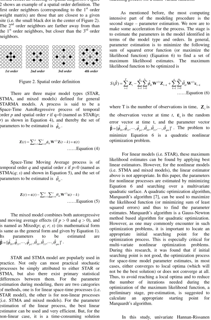
should reflect an ordering of spatial neighbors. Figure 2 shows an example of a spatial order definition. The first order neighbors (corresponding to the 1st order weight matrix) are those that are closest to a given site (i.e. the small black dot in the center of Figure 2).
The 2nd order neighbors are farther away from than the 1st order neighbors, but closer than the 3rd order neighbors.
1st order 2nd order 3rd order 4th order
Figure 2. Spatial order definition
There are three major model types (STAR, STMA, and mixed models) defined for general STARMA models. A process is said to be a Space-Time AutoRegressive process of temporal order p and spatial order r if q=0 (named as STAR(p;
r) as shown in Equation 4), and thereby the set of parameters to be estimated is φˆkl.
) ( ) ( )
( 1 0
)
( t k t
t p
k r l
l
klW Z ε
Z =
∑ ∑
= =φ − +……Equation (4) Space-Time Moving Average process is of temporal order q and spatial order s if p=0 (named as STMA(q; s) and shown in Equation 5), and the set of parameters to be estimated is θˆkl.
∑ ∑
= = −−
= q
k s l
l
kl t k
t
t 1 0
)
( ( )
) ( )
( ε W ε
Z θ
……Equation (5) The mixed model combines both autoregressive and moving average effects (if p > 0 and q > 0), and is named as Mixed(p; q; r; s) (its mathematical form is same as the general form and given by Equation 1).
Its parameters to be estimated are .
t 11
10 11
10 ,ˆ , ,ˆ ,ˆ ,ˆ , ,ˆ ] [ˆ
ˆ= φ φ Lφpλ θ θ Lθqm
β
STAR and STMA model are popularly used in practice. Not only can most practical stochastic processes be simply attributed to either STAR or STMA, but also there exist primary statistical differences between them. For the parameter estimation during modeling, there are two categories of methods, one is for linear space-time processes (i.e.
STAR model), the other is for non-linear processes (i.e. STMA and mixed models). For the parameter estimation of the linear process, the best linear estimator can be used and very efficient. But, for the non-linear case, it is a time-consuming solution
searching process for a multi-variate function.
As mentioned before, the most computing intensive part of the modeling procedure is the second stage – parameter estimation. We now are to make some acceleration for the process. The stage is to estimate the parameters in the model identified in terms of the model type and orders. In general, parameter estimation is to minimize the following sum of squared error function (or maximize the likelihood function) (Equation 6) to find a set of maximum likelihood estimates. The maximum likelihood function to be optimized is
∑∑
∑ ∑∑
= = −
= − = = − +
= q
k m
l
k t l kl T
t
p
k l
k t l kl t
k k
S
1 0
) (
1 1 0
)
( ˆ
) ˆ
(βˆ Z λ φ W Z θ W ε
……Equation (6)
where T is the number of observations in time, is the observation vector at time t, is the random error vector at time t, and the parameter vector . The problem to minimize Equation 6 is a quadratic nonlinear optimization problem.
Zt
εt
t 11
10 11
10 ,ˆ , ,ˆ ,ˆ ,ˆ , ,ˆ ] [ˆ
ˆ= φ φ Lφpλ θ θ Lθqm
β
For linear models (i.e. STAR), these maximum likelihood estimates can be found by applying best linear estimators. However, for the nonlinear models (i.e. STMA and mixed models), the linear estimator above is not appropriate. In this paper, the parameters for nonlinear processes are estimated by minimizing Equation 6 and searching over a multivariate quadratic surface. A quadratic optimization algorithm, Marquardt’s algorithm [7], can be used to maximize the likelihood function (or minimizing sum of least squared errors) and thus to find the parameter estimates. Marquardt’s algorithm is a Gauss-Newton method based algorithm for quadratic optimization.
However, as one may commonly encounter in such optimization problems, it is important to locate an appropriate initial searching point for the optimization process. This is especially critical for multi-variate nonlinear optimization problems.
During this research, it was found that if initial searching point is not good, the optimization process for space-time model parameter estimates, in most cases, either converges to local optima (which will not be the best solution) or does not converge at all.
Thus, to avoid reaching a local optima and to reduce the number of iterations needed during the optimization of the maximum likelihood function, a preliminary stage, pre-estimation, is suggested to calculate an appropriate starting point for Marquardt’s algorithm.
In this study, univariate Hannan-Rissanen
algorithm[5] has been extended to the multivariate STARMA series as shown below. The space-time extension of Hannan-Rissanen algorithm has three iterative steps:
Step 1. A high order STAR model is fitted to the data using the space-time Yule-Walker equations. Then, we have the following approximate model
*
1 0
* ) (
* ˆ t
u
k v
l
k t l kl
t W Z ε
Z =
∑∑
+= = η −
where {ηˆkl|k=1,L,u;l=0,L,v} are the Yule-Walker estimates.
Step 2. The estimated random noise vectors can be found as
∑∑
= = −−
=
≡ u
k v
l
k t l kl t
t t
1 0
* ) (
*
* ˆ
ˆ ε Z W Z
ε η
……Equation (3) Step 3. Once the estimated random noise vectors εˆ , t t=m+1, …, T, have been found from Equation 3, pre-estimates for the model parameters,
are determined by the least squares linear regression of projecting onto the space {Zt-1, Zt-2, …, Zt-p,
t t t,ˆ ] [ˆ
ˆ ϕ ψ
α=
Zt
ˆt−1
ε , εˆt−2, …, εˆt−q}, t=m+1, …, T.
By minimizing the sum of squared errors
∑ ∑∑ ∑∑
+
= = = −
= = − ⎟⎟⎠
⎞2
⎜⎜⎝
⎛ − +
= T
m t
q
k m
l
k t l kl p
k l
k t l kl t
k k
S
1 1 0
) (
1 0
)
( ˆ
) ˆ
(αˆ Z λ ϕ W Z ψ W εˆ
with respect to αˆ
( )
Ω= XtX −1Xt αˆ
, we can obtain the space-time extension of the Hannan-Rissanen estimator as
where
, ˆ ] , ˆ , ˆ , ˆ , , ˆ , ˆ ,
ˆ [ϕ10 ϕ11 ϕklψ10ψ11 ψkl t
α= L L
, ] , , ,
[Zm+1 Zm+2L ZT t
= Ω
⎢⎢
⎢⎢
⎢
⎣
⎡
=
−
−
−
−
−
+ +
+
−
−
2 ) ( 2
1 ) ( 1
) 1 ( 1
) ( 1
) ( 1
) 1 ( 1
1 ) ( 1
) ( )
1 (
T r T
T r T
T
m r m
m r m
m
m r m
m r m
m
Z W Z
Z W Z
W Z
Z W Z
Z W Z
W Z
Z W Z
Z W Z
W Z X
L L
M L M M
L M M
L L
L L
L L L L
⎥⎥
⎥⎥
⎥
⎦
⎤
−
−
−
−
−
+ +
+
−
−
2 ) ( 2
1 ) ( 1
) 1 ( 1
) ( 1
) ( 1
) 1 ( 1
1 ) ( 1
) ( )
1 (
ˆ ˆ
ˆ ˆ
ˆ
ˆ ˆ
ˆ ˆ
ˆ
ˆ ˆ
ˆ ˆ
ˆ
T r T
T r T
T
m r m
m r m
m
m r m
m r m
m
W W
W
W W
W
W W
W
ε ε
ε ε
ε
ε ε
ε ε
ε
ε ε
ε ε
ε
L L
M L M M L M M
L L
L L
.
Discussion
From simulation results, the space-time extension of Hannan-Rissanen algorithm is very efficient and robust. The deviations of the parameter pre-estimates αˆ from the expected values are generally lower than 10%.
This algorithm greatly reduces the possibility of converging to a local optima or diverging and hence improves the robustness of the modeling process.
Combining with the space-time extensions of STARMA model fitness measures, e.g. Akaike’s information criterion (AIC) and Bayesian information criterion (BIC), we can make the entire modeling iterative procedure automatic and accurate.
Reference
1. Box, G. E. P. and Jenkins, G. M. (1970). Time Series Analysis: Forecasting and Control.
Holden-Day, San Francisco.
2. Cliff, A. D., Haggett, P., Ord, J. K., Bassett, K. A.
and Davies, R. B. (1975). Elements of Spatial Structure: A Quantitative Approach. Cambridge University Press, New York.
3. Cliff, A. D. and Ord, J. K.. Model building and the analysis of spatial pattern in human geography. Journal of the Royal Statistical Society Series B, 37:297-348,1975.
4. Epperson, B. K. Spatial and space-time correlations in ecological models. Ecol Modell 132, 63-76, 2000.
5. Hannan, E.J. and Rissanen, J. Recursive estimation of mixed auto-regressive moving average order. Biometrika, 69:81-94, 1982.
6. Hay, et al. Climate change and the resurgence of malaria in the East African highlands, Nature, Vol.415, 2002.
7. Marquardt, D.W. An algorithm for least squares estimation of nonlinear parameters. Journal of the Society of Industrial and Applied Mathematics, 11:431-441, 1963.
8. Martin, R.L. and Oeppen, J. E. The identification of regional forecasting models using space-time correlation functions. Transactions of the Institute of British Geographers, 66:95-118, 1975.
9. Petersen, L. and Roehrig, J. West Nile virus: a reemerging global pathogen. Emerging Infectious Diseases, 7(4):611-614, 2001.
10. Pfeifer, P. E. Spatial-Dynamic Modeling (Unpublished Ph.D. dissertation). Georgia Institute of Technology, Atlanta, Georgia, 1979.
11. Pfeifer, P.E. and Deutsch, S.J. A three-stage iterative procedure for space-time modeling.
Technometrics 22(1), 35-47, 1980.
12. Pfeifer, P.E. and Deutsch, S.J. A comparison of estimation procedures for the parameters of the STAR model. Communications in Statistics - Simulation and Computation, B9 (3):255-270, 1980.