行政院國家科學委員會補助專題研究計畫成果報告
※※※※※※※※※※※※※※※※※※※※※※※※※
※ ※
※ 一個推估多項目量表內部一致性之無母數方法 ※
※ ※
※※※※※※※※※※※※※※※※※※※※※※※※※
計畫類別:■個別型計畫 □整合型計畫
計畫編號:NSC 89-2314-B-006-150-
執行期間:89 年 08 月 01 日至 91 年 01 月 31 日
計畫主持人: 王新台 教授
本成果報告包括以下應繳交之附件:
□赴國外出差或研習心得報告一份
□赴大陸地區出差或研習心得報告一份
□出席國際學術會議心得報告及發表之論文各一份
□國際合作研究計畫國外研究報告書一份
執行單位:國立成功大學醫學院公共衛生科
中 華 民 國 91 年 01 月 09 日
行政院國家科學委員會專題研究計畫成果報告
計畫編號:NSC 89-2314-B-006-150
執行期限:89 年 08 月 01 日至 90 年 07 月 31 日
主持人:王新台 教授
執行機構及單位名稱:國立成功大學醫學院公共衛生科
中文摘要 在這份報告中,我們在假設兩因子混合模型 情況下,電腦模擬比較一個母數和一個無母 數估計量表內部一致性之方法。這裡的內部 一致性是由 Kendall’s tau 相關係數延伸而 來,比起 Cronbach’s alpha 解釋上較簡單。 我們推導了兩種估計方法之變異數的公 式。模擬中計算了兩種估計方法之偏差量、 根號的平均平方差,以及信賴區間包含機 率,並加以比較。模擬結果發現根號的平均 平方差會隨著題數的增加或者是測驗信度 的增加而減少。無母數估計方法,在樣本數 足夠的情況下,與母數估計法一樣好。但是 仍需近一了解,在不符合兩因子混合模型情 況下,兩者統計性質。 關鍵詞:模擬、內部一致性 AbstractA simulations study was undertaken to compare a model-based and a sample-based estimators of a new index for internal consistency under a two-factor (subject by item). This new index is essentially a generalization of Kendall’s tau correlation coefficient and has a simpler interpretation than Cronbach’s alpha. Variance formulae for the model-based and sample-based estimators were derived. Biases, root mean square errors (RMSE), and coverage probabilities of these estimators were calculated and compared. The RMSE decreases as the number of test items
increases or as the test reliability increases. The results show that the sample-based estimator performs equally well as the model-based estimator when the number of subjects increases. However, further
investigation is needed to study their
performance when the assumptions embedded in the two-factor model are violated.
Keywords: Simulation, internal consistency
Background
Internal consistency is among one of the major concerns while developing a test instrument or questionnaire with multiple items that are intended to measure a unidimensional attribute. The associated degree of internal consistency refers to the extend to which the items that make up the instrument are parallel measurement An instrument that is intended to measure a single attributed should be devised to reflect an adequate degree of internal consistency, so that the attribute could be consistently estimated by a parsimonious set of items. Cronbach’s alpha (Cronbach, 1951) is the most widely used index for measuring internal consistency. However, the index can render negative values that defy interpretation and does not take account of multidimension in a set of items. Moreover, its interpretation as the average of all the possible split-half
coefficients of a test is somewhat mysterious to applied researchers. We described internal consistency by a joint probability that is essentially a generalization of Kendall’s tau correlation coefficient (Hollander & Wolfe, 1973). The idea originates from an intuitive notion about internal consistency. Basically it is assumed that as the homogeneity of a test increases, a test taker with a higher total-test score should have a greater probability of obtaining a higher score on each and every item than a test taker with a lower total-test score (Anastasi, 1988, p123). Both a model-based estimator and a sample-based estimator were proposed to estimate the joint probability (Wang, NSC87-2416-H-006-034). However, the variance formulae for these estimators were not derived. In this report, we proposed a variance formula for the
model-based estimator under a two-factor (subject by item) mixed effects model and a large-sample variance formula for the sample-based estimator derived under the
U-statistics theory. A monte-carlo simulation
was undertaken to study the performance of both the estimators under a two-factor
(subject by item) mixed effects model. It is of particular interest to compare the
sample-based estimator to the model-based estimator.
Results
The new measure of internal consistency, denoted by ϕ, under a two-factor (subject by item) mixed effects model (Feldt, 1965) given by Yij = µ + aj+ ti + eij , where = 0, ∼ N(0, ), and ∼N(0, ) (1)
∑
= k j j a 1 i t 2 t σ /( 1 k ij e σe2σ
/ ) 1 m P ^ g ∂ ∂ g m ^ ϕ 2 ) j i Y ,' /( ) 2 k− − k) ,..., i i I [ = < 2 (n n P ^ ) is defined as ϕ = P = {2E ) 1 − z[(1- Φ(z× r ))k]} ) 1 /( 1 k−whereΦ(u) is the cumulative distribution function of a standard normal variate evaluated at u, Ez is an expectation over a standard normal variate z and r
(=
t
2
σ
)is test reliability. Using the delta-method, we could derive an estimated variance of the model-based estimator given as e 2 m ^ ϕ = Pm ={2E ^ 1/(k− z[(1-Φ(z× ^ r )) ]} k 1/(k−1)as follows. Note that
Var( ) ≅ 2 2 2 ) ) ( ( r r ×Var( ^ r2)
where = 2E(r2) z[(1- Φ(z× r )) ]. Using the delta-method, k Var( ) ≅ ^ ^ ) ( 1 ( Pm2( 1) Var Pm k k × ×
Ninety-five percent confidence limits were derived in a previous report (Wang,
NSC87-2416-H-006-034).
An unbiased sample estimator of P is given as s P ^ n
∑∑
= s j i ij i ij j I Y Y j k N Y 1 ( , 1,..., )]/ ( ' 1 ' = < + = > where Ns= −1) .The corresponding estimator for ϕ can be
written as = . An estimated
variance of can be derived as
s ^ ϕ s 1 /( 1 k− s P ^
Var(Ps) = ^ 2 1 { ) 1 ( 4 − n n P- 2) 3 − n ( P2 +(n−2)B(12)(13)} where ) 13 )( 12 ( B ( ( 2 2 Y P Y P r j r + = ). ,..., 1 , , ( ) ,..., 1 , , ( ) ,..., 1 , , 1 3 1 2 1 3 1 1 2 1 3 1 k j Y Y Y Y P k j Y Y Y Y Y P k j Y Y Y j j j j r j j j j j j r j j j = < < + = > < > + = > > ,Y3j <Y1j, j =1,..,k)
For each case, ϕ was calculated and 2000 trials were generated. For each trial, , ,
, and 95 percent confidence limits were obtained. The biases, root mean square errors (RMSE), and coverage probabilities of these estimators were also computed. The estimated variances of and were also calculated and compared to simulated variances to check the adequacy of the variance formulae. m ^ ϕ Pm ^ s ^ ϕ Ps ^ m P ^ s P ^
Using the delta-method,
Var( s) ^ ϕ ≅ 2 ^ ^ ) ( ) 1 ( Ps2( 2)/( 1) Var Ps k k k × × − − .
According to the U-statistics theory,
N(P, Var( )) as Ninety
percent confidence limits were computed based on this large sample result.
→ s P ^ s P ^ . ∞ → 思n
A simulation study was carried out to investigate the performance of the proposed model-based and model-based estimators under the mixed effects model (1). The
number of test examinees ( ) was set to be 25, 50, or 100, and the number of test items ( ) was chosen to be 10, 15, 20. Without loss of generality,
n
k
µ was chosen to be 3, and six cases of and as follows were considered. 2 t σ 2 e σ Case 1: σt2=5, and σe2=2.5 (r2= 2), Case 2: σt2=5, and σe2= 1.25 (r2= 4), Case 3: σt2=5, and σe2= 0.833 (r2= 6), Case 4: σt2=5, and σe2= 0.625 (r2= 8), Case 5: σt2=5, and σe2= 0.5 (r2= 10), and Case 6: σt2=5, and σe2= 0.417 (r2= 12).
Tables 1, 2 and 3 show the results of the simulation when =25. The estimated
variances of the and were comparable to the corresponding simulated variances. Both the and slightly underestimate ϕ in all
the cases, but has smaller biases. The , on the other hand, has smaller RMSE and more satisfactory coverage probabilities. However, the differences in RMSE between the two estimators were small. As
increases to 50 or 100, the biases, and RMSE of the sample-based estimator become
negligible and the coverage probabilities were closer to 95 percent (data not shown). More important, they fared equally well with those of the model-based estimator.
n m P ^ s s P ^ m ^ ϕ ϕ^s ^ ϕ ϕ^m n
probabilities of and for the various and
m
^
ϕ ϕ^s
k r2 when =25. The RMSE for the both the estimators of ϕ are decreasing in
and
n
k r2and the coverage probabilities for the sample-based estimator tend to decrease when
2
r increases. The same findings were obtained when n=50 or n=100.
Discussion
The estimated variances of and were of the same magnitudes as the
corresponding simulated variances. But the estimated variances of and were in some cases 10 times smaller than the corresponding simulated variances. The discrepancies could be partly due to the functional form of and ,
and raised to m P ^ s s P ^ m ^ ϕ ϕ^ m ^ ϕ ϕ^s m P ^ s P ^ th 1 1 − n k power, that
rendered the first-order Taylor’s expansion inadequate or be partly attributed to pure simulation glitches. As increases, the differences subsided.
The coverage probabilities of the sample-based estimator improved as increases, validating the large sample normality. It appears that the sample-based estimator has smaller coverage probabilities for larger inter-item correlations. In other words, the normality of the sample-based estimator will be affected by the magnitudes of the inter-item correlations.
n
The sample-based estimator performed equally well as the model-based estimator when the sample size is sufficiently large under the two-factor model (1), and does not require numerical integration. As a matter fact, it can be programmed easily in SAS or
Fortran. Further investigation is needed to study their performance when the assumptions embedded in the two-factor model are
violated.
References
Anastasi, A. (1988). Psychological Testing. New York: Macmillan Publishing Company.
Cronbach, L. J. (1951). Coefficient alpha and the internal structure of tests.
Psychometrika, 16, 297-334.
Feldt, L. S. (1965). The approximate sampling distribution of Kuder-Richardson reliability coefficient twenty.
Psychometrika, 30, 357-379. Hollander, M. and Wolfe, D. A. (1973).
Nonparametric Statistical Methods. New York: John Wiley and Sons. Wang, S.T. (1998). A New Index for
Measuring Internal Consistency of Multiple-item Instruments. National Science Council Archives,
0 2 4 6 8 10 12 0.00 0.01 0.02 0.03 0.04 0.05 Model-based method (k=10) Sample-based method (k=10) Model-based method (k=15) Sample-based method (k=15) Model-based method (k =20) Sample-based method (k =20) r2 Ro ot mea n s q u ar e erro r fo r esti mat in g ϕ 0 2 4 6 8 10 12 0.85 0.86 0.87 0.88 0.89 0.90 0.91 0.92 0.93 0.94 0.95 0.96 r2 Co v er a g e pr o b a bil it ie s
Figure 1. The root mean square errors and coverage probabilities for the model-based and sample-based estimators
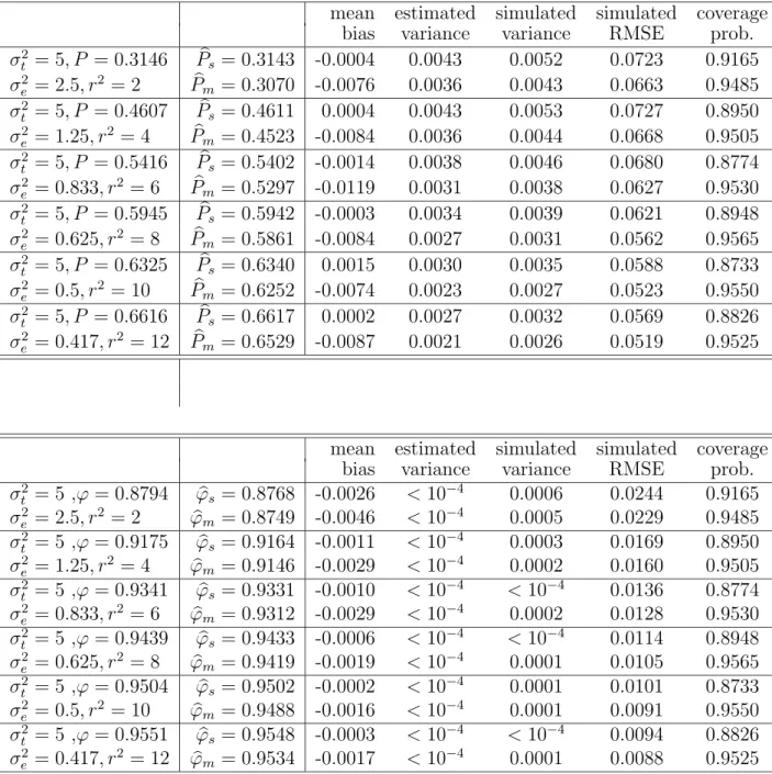
Table 1 Comparison of the sample-based estimator and the model-based estimator based on continuous score data. (µ = 3, n=25, k=10)
mean estimated simulated simulated coverage
bias variance variance RMSE prob.
σ2 t = 5, P = 0.3146 Pbs = 0.3143 -0.0004 0.0043 0.0052 0.0723 0.9165 σ2 e = 2.5, r2 = 2 Pbm = 0.3070 -0.0076 0.0036 0.0043 0.0663 0.9485 σ2 t = 5, P = 0.4607 Pbs = 0.4611 0.0004 0.0043 0.0053 0.0727 0.8950 σ2 e = 1.25, r2 = 4 Pbm = 0.4523 -0.0084 0.0036 0.0044 0.0668 0.9505 σ2 t = 5, P = 0.5416 Pbs = 0.5402 -0.0014 0.0038 0.0046 0.0680 0.8774 σ2 e = 0.833, r2 = 6 Pbm = 0.5297 -0.0119 0.0031 0.0038 0.0627 0.9530 σt2 = 5, P = 0.5945 Pbs = 0.5942 -0.0003 0.0034 0.0039 0.0621 0.8948 σe2 = 0.625, r2 = 8 Pbm = 0.5861 -0.0084 0.0027 0.0031 0.0562 0.9565 σt2 = 5, P = 0.6325 Pbs = 0.6340 0.0015 0.0030 0.0035 0.0588 0.8733 σe2 = 0.5, r2 = 10 Pbm = 0.6252 -0.0074 0.0023 0.0027 0.0523 0.9550 σ2 t = 5, P = 0.6616 Pbs = 0.6617 0.0002 0.0027 0.0032 0.0569 0.8826 σ2 e = 0.417, r2 = 12 Pbm = 0.6529 -0.0087 0.0021 0.0026 0.0519 0.9525
mean estimated simulated simulated coverage
bias variance variance RMSE prob.
σ2 t = 5 ,ϕ = 0.8794 ϕbs= 0.8768 -0.0026 < 10 −4 0.0006 0.0244 0.9165 σe2 = 2.5, r2 = 2 ϕbm = 0.8749 -0.0046 < 10−4 0.0005 0.0229 0.9485 σ2 t = 5 ,ϕ = 0.9175 ϕbs= 0.9164 -0.0011 < 10 −4 0.0003 0.0169 0.8950 σe2 = 1.25, r2 = 4 ϕbm = 0.9146 -0.0029 < 10−4 0.0002 0.0160 0.9505 σ2 t = 5 ,ϕ = 0.9341 ϕbs= 0.9331 -0.0010 < 10−4 < 10−4 0.0136 0.8774 σe2 = 0.833, r2 = 6 ϕbm = 0.9312 -0.0029 < 10−4 0.0002 0.0128 0.9530 σt2 = 5 ,ϕ = 0.9439 ϕbs= 0.9433 -0.0006 < 10−4 < 10−4 0.0114 0.8948 σe2 = 0.625, r2 = 8 ϕbm = 0.9419 -0.0019 < 10 −4 0.0001 0.0105 0.9565 σt2 = 5 ,ϕ = 0.9504 ϕbs= 0.9502 -0.0002 < 10−4 0.0001 0.0101 0.8733 σ2 e = 0.5, r2 = 10 ϕbm = 0.9488 -0.0016 < 10 −4 0.0001 0.0091 0.9550 σt2 = 5 ,ϕ = 0.9551 ϕbs= 0.9548 -0.0003 < 10−4 < 10−4 0.0094 0.8826 σ2 e = 0.417, r2 = 12 ϕbm = 0.9534 -0.0017 < 10 −4 0.0001 0.0088 0.9525 7
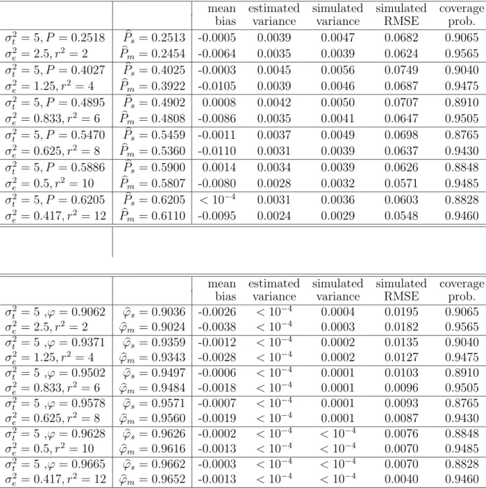
Table 2 Comparison of the sample-based estimator and the model-based estimator based on continuous score data. (µ = 3, n=25, k=15)
mean estimated simulated simulated coverage
bias variance variance RMSE prob.
σ2 t = 5, P = 0.2518 Pbs = 0.2513 -0.0005 0.0039 0.0047 0.0682 0.9065 σ2 e = 2.5, r2 = 2 Pbm = 0.2454 -0.0064 0.0035 0.0039 0.0624 0.9565 σ2 t = 5, P = 0.4027 Pbs = 0.4025 -0.0003 0.0045 0.0056 0.0749 0.9040 σ2 e = 1.25, r2 = 4 Pbm = 0.3922 -0.0105 0.0039 0.0046 0.0687 0.9475 σ2 t = 5, P = 0.4895 Pbs = 0.4902 0.0008 0.0042 0.0050 0.0707 0.8910 σ2 e = 0.833, r2 = 6 Pbm = 0.4808 -0.0086 0.0035 0.0041 0.0647 0.9505 σt2 = 5, P = 0.5470 Pbs = 0.5459 -0.0011 0.0037 0.0049 0.0698 0.8765 σe2 = 0.625, r2 = 8 Pbm = 0.5360 -0.0110 0.0031 0.0039 0.0637 0.9430 σt2 = 5, P = 0.5886 Pbs = 0.5900 0.0014 0.0034 0.0039 0.0626 0.8848 σe2 = 0.5, r2 = 10 Pbm = 0.5807 -0.0080 0.0028 0.0032 0.0571 0.9485 σ2 t = 5, P = 0.6205 Pbs = 0.6205 < 10−4 0.0031 0.0036 0.0603 0.8828 σ2 e = 0.417, r2 = 12 Pbm = 0.6110 -0.0095 0.0024 0.0029 0.0548 0.9460
mean estimated simulated simulated coverage
bias variance variance RMSE prob.
σ2 t = 5 ,ϕ = 0.9062 ϕbs= 0.9036 -0.0026 < 10 −4 0.0004 0.0195 0.9065 σe2 = 2.5, r2 = 2 ϕbm = 0.9024 -0.0038 < 10−4 0.0003 0.0182 0.9565 σ2 t = 5 ,ϕ = 0.9371 ϕbs= 0.9359 -0.0012 < 10 −4 0.0002 0.0135 0.9040 σe2 = 1.25, r2 = 4 ϕbm = 0.9343 -0.0028 < 10−4 0.0002 0.0127 0.9475 σ2 t = 5 ,ϕ = 0.9502 ϕbs= 0.9497 -0.0006 < 10−4 0.0001 0.0103 0.8910 σe2 = 0.833, r2 = 6 ϕbm = 0.9484 -0.0018 < 10−4 0.0001 0.0096 0.9505 σt2 = 5 ,ϕ = 0.9578 ϕbs= 0.9571 -0.0007 < 10−4 0.0001 0.0093 0.8765 σe2 = 0.625, r2 = 8 ϕbm = 0.9560 -0.0019 < 10 −4 0.0001 0.0087 0.9430 σt2 = 5 ,ϕ = 0.9628 ϕbs= 0.9626 -0.0002 < 10−4 < 10−4 0.0076 0.8848 σ2 e = 0.5, r2 = 10 ϕbm = 0.9616 -0.0013 < 10 −4 < 10−4 0.0070 0.9485 σt2 = 5 ,ϕ = 0.9665 ϕbs= 0.9662 -0.0003 < 10−4 < 10−4 0.0070 0.8828 σ2 e = 0.417, r2 = 12 ϕbm = 0.9652 -0.0013 < 10 −4 < 10−4 0.0040 0.9460 8
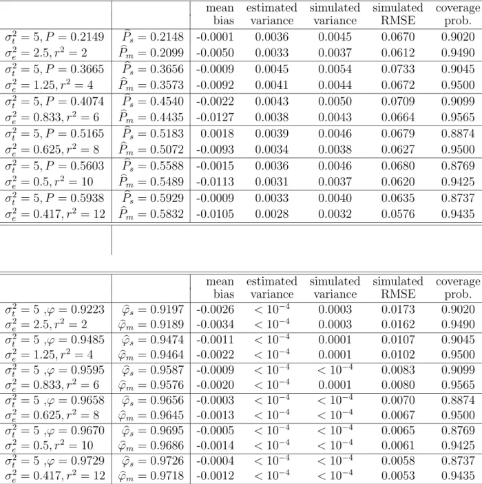
Table 3 Comparison of the sample-based estimator and the model-based estimator based on continuous score data. (µ = 3, n=25, k=20)
mean estimated simulated simulated coverage
bias variance variance RMSE prob.
σ2 t = 5, P = 0.2149 Pbs = 0.2148 -0.0001 0.0036 0.0045 0.0670 0.9020 σ2 e = 2.5, r2 = 2 Pbm = 0.2099 -0.0050 0.0033 0.0037 0.0612 0.9490 σ2 t = 5, P = 0.3665 Pbs = 0.3656 -0.0009 0.0045 0.0054 0.0733 0.9045 σ2 e = 1.25, r2 = 4 Pbm = 0.3573 -0.0092 0.0041 0.0044 0.0672 0.9500 σ2 t = 5, P = 0.4074 Pbs = 0.4540 -0.0022 0.0043 0.0050 0.0709 0.9099 σ2 e = 0.833, r2 = 6 Pbm = 0.4435 -0.0127 0.0038 0.0043 0.0664 0.9565 σt2 = 5, P = 0.5165 Pbs = 0.5183 0.0018 0.0039 0.0046 0.0679 0.8874 σe2 = 0.625, r2 = 8 Pbm = 0.5072 -0.0093 0.0034 0.0038 0.0627 0.9500 σt2 = 5, P = 0.5603 Pbs = 0.5588 -0.0015 0.0036 0.0046 0.0680 0.8769 σe2 = 0.5, r2 = 10 Pbm = 0.5489 -0.0113 0.0031 0.0037 0.0620 0.9425 σ2 t = 5, P = 0.5938 Pbs = 0.5929 -0.0009 0.0033 0.0040 0.0635 0.8737 σ2 e = 0.417, r2 = 12 Pbm = 0.5832 -0.0105 0.0028 0.0032 0.0576 0.9435
mean estimated simulated simulated coverage
bias variance variance RMSE prob.
σ2 t = 5 ,ϕ = 0.9223 ϕbs= 0.9197 -0.0026 < 10 −4 0.0003 0.0173 0.9020 σe2 = 2.5, r2 = 2 ϕbm = 0.9189 -0.0034 < 10−4 0.0003 0.0162 0.9490 σ2 t = 5 ,ϕ = 0.9485 ϕbs= 0.9474 -0.0011 < 10 −4 0.0001 0.0107 0.9045 σe2 = 1.25, r2 = 4 ϕbm = 0.9464 -0.0022 < 10−4 0.0001 0.0102 0.9500 σ2 t = 5 ,ϕ = 0.9595 ϕbs= 0.9587 -0.0009 < 10−4 < 10−4 0.0083 0.9099 σe2 = 0.833, r2 = 6 ϕbm = 0.9576 -0.0020 < 10−4 0.0001 0.0080 0.9565 σt2 = 5 ,ϕ = 0.9658 ϕbs= 0.9656 -0.0003 < 10−4 < 10−4 0.0070 0.8874 σe2 = 0.625, r2 = 8 ϕbm = 0.9645 -0.0013 < 10 −4 < 10−4 0.0067 0.9500 σt2 = 5 ,ϕ = 0.9670 ϕbs= 0.9695 -0.0005 < 10−4 < 10−4 0.0065 0.8769 σ2 e = 0.5, r2 = 10 ϕbm = 0.9686 -0.0014 < 10 −4 < 10−4 0.0061 0.9425 σt2 = 5 ,ϕ = 0.9729 ϕbs= 0.9726 -0.0004 < 10−4 < 10−4 0.0058 0.8737 σ2 e = 0.417, r2 = 12 ϕbm = 0.9718 -0.0012 < 10 −4 < 10−4 0.0053 0.9435 9