行政院國家科學委員會專題研究計畫成果報告 正交函數近似法用於不確定性撓性關節機械臂之適應控制研究
Adaptive Contr ol of Uncer tain Flexible J oint Robot Using Or thonor mal Function Appr oximation
計畫編號:NSC 90-2212-E-011-056 執行期限:90 年 8 月 1 日至 91 年 7 月 31 日 主持人: 黃安橋 國立台灣科技大學機械系
中文摘要
本計畫對一具有未知邊界時變未知參數之單桿撓軸 機械臂,提出適應控制法則。未知參數係於回授線性化 領域中,以正交函數之有限組合進行近似。一適應控制 器則被設計成得以確保追蹤誤差之漸近收斂;同時,諸 時變未知參數之估測值亦皆為有界。為測試本計畫所提 控制器之性能,除嚴謹數學證明外,亦進行電腦模擬,
以及實驗。實驗所需之單桿撓軸機械臂,係一併於本計 畫中設計與製作。模擬與實驗結果顯示,本計畫所發展 之控制器確實可達到預期之效果。
關鍵字:適應控制,撓性關節機械臂,函數近似。
Abstr act
A sliding control based adaptive controller is proposed in this project for a single-link flexible-joint robot. The lumped uncertainties represented in the feedback-linearized domain are assumed to be time-variant and their variation bounds are not given. Since the conventional robust designs or adaptive strategies can not be applied directly, the function approximation technique is used to represent those uncertain terms into linearly parameterized forms. The form is basically an inner product of a known basis function vector and an unknown coefficient vector. Since the coefficient vector is time-invariant, an update law can be easily derived from the traditional Lyapunov design.
Convergence of the output error and boundedness of internal signals are proved under the assumption of proper selection of basis functions. Experiment results justify the usefulness of the proposed scheme.
Keywor ds: Flexible joint robot, adaptive control, function approximation.
1. Intr oduction
Many industrial robots use harmonic drives to reduce speed and amplify output torque. A cup-shape component in the harmonic drive provides elastic deformation to enable large speed reduction. Therefore, it is known that harmonic drives introduce torsional flexibility into the robot joints. To have a high performance robot control system, elastic coupling between actuators and links cannot be neglected.
Modeling of these effects, however, produces an enormously complicated model. For simplicity, let us consider a single-link flexible-joint robot that can be modeled by inserting a linear torsional spring between the shaft of the motor and the end about which the link is rotating. Two second-order differential equations should be used to describe its dynamic behavior, one for the motor shaft and one for the link. This implies that the number of degree-of-freedom is twice the number for a rigid robot, since the motion of the motor shaft is no longer simply
related to the link angle by the gear ratio. Because the model inevitably contains inaccuracies, any practical design should consider their effects. The highly nonlinear coupling and model inaccuracies make the controller design for a flexible joint robot extremely difficult. Based on the assumption that the fast part of the robot dynamics is much faster than the slower part, the singular perturbation technique was proposed to stabilize the system [11,17]. A fast joint torque control loop and a slower output control loop were designed in this approach. However, the strategy can only be applied to robots with weak joint flexibility. Spong [20] proposed a feedback linearization based controller for precisely known flexible joint robots. Several controllers were designed [1,15,10] for the flexible joint robot with full state feedback.
To reduce the number of sensors for measuring system states and to avoid possible measuring noise, various controllers were proposed with partial state feedback [14,13,16,3]. For considering modeling inaccuracies, robust controllers were designed [2,23,16]. Adaptive controllers for flexible joint robots with fixed structure and unknown constant parameters were also suggested [5,6,12,24,13,4]. In this project, an adaptive sliding controller is suggested for a single-link flexible-joint robot. In the feedback-linearized domain, the lumped uncertainties are assumed to be represented as functions of time and their variation bounds are not given.
Hence, conventional robust control or adaptive strategies are not applicable directly. The function approximation technique [7,8,9] is employed to transform the uncertain terms into linearly parameterized forms. The form is basically an inner product of a known basis function vector and an unknown coefficient vector. Since the coefficient vector is time-invariant, we may use traditional Lyapunov stability theory to derive its update law to have convergence of the output error and boundedness of internal signals.
This report is organized as follows. Section 2 reviews some concepts of function approximation with orthonormal basis functions. Section 3 presents the derivation of the proposed controller. Experiment results are shown in section 4.
2. Review of or thonor mal function appr oximation
In this section some basic notions of function approximation with orthonormal functions are reviewed. Let us consider a set of functions {bi(t)} that are orthonormal in [t1, t2] such that
∫12 =1, =≠ , ) 0 ( ) ( *
t
t i j
j i
j dt i
t b t
b (1)
where ()* denotes the complex conjugate operator. With the definition of the inner product < >=∫12
) ( ) (
, t *
t f t g t dt g
f
and its corresponding norm f = < f,f >, the space of
functions for which f exists and is finite is a Hilbert space [22,18]. If {bi(t)} is an orthonormal basis in the sense of (1) then every f(t) with f finite can be expanded in the form
∑∞
=
=
1
) ( )
(
i i ib t w t
f (2)
where wi =< f,bi> is the Fourier coefficient, and the series converges in the sense of mean square as
∫ −∑ =
∞ =
→
2
1
0 ) ( )
( lim
2
1 t
t
n
i i
n f t wib t dt . (3)
This implies that any function f(t) in the current Hilbert space can be approximated to arbitrarily prescribed accuracy by finite linear combinations of the orthonormal basis {bi(t)}
as
∑=
≈ n
i i ib t w t f
1
) ( )
( . (4)
An excellent property of (4) is its linear parameterization of the time-varying function f(t) into a basis function vector
T n t b t
b t b
t) [ () () ()]
( = 1 2 L
b and a time-invariant
coefficient vector w=[w1 w2 L wn]T , i.e.,f(t)≈wTb(t). We would like to abuse the notation by writing the approximation as f(t)=wTb(t) provided a sufficient number of the basis functions is used. In the next section, equation (4) is used to represent the time-varying parameter in the system dynamic equation. The time-varying vector b(t) is known while w is an unknown constant vector.
With this approximation, the unknown time-varying function is replaced by a set of unknown constants; therefore, a proper Lyapunov function can be selected to find update laws for these unknown constants.
3. Main Results
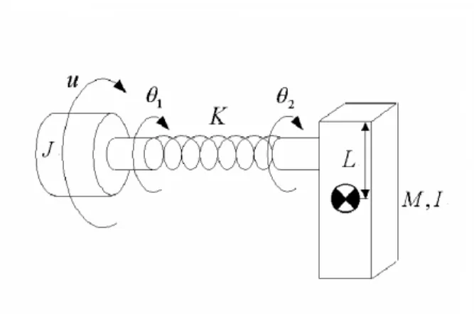
Let us consider a single-link flexible-joint robot (Figure 1) rotating in a vertical plane with the assumptions that its joint can only deform in the direction of joint rotation, the link is rigid, the viscous damping is neglected, and the states are measurable. The dynamic equation of the robot is given by [19]
1 3 1 4
4 3
3 1 1 2
2 1
) 1 (
) ( sin
x y
J u x J x x k
x x
x I x x k I x mgl
x x
=
+
−
=
=
−
−
−
=
=
&
&
&
&
(5)
in which xi∈ℜ, i=1,...,4 are state variables, and the output y is equal to the link displacement. The link inertial I, the rotor inertia J, the stiffness k, the link mass m, the gravity constant g, and the center of mass l are positive parameters.
The control u is the torque delivered by the motor. The system equation can be further written in the standard affine form
) (
) ( ) (
x x g x f x
h y
u
= +
=
&
(6)
where
1
3 1 4 3 1 1 2
4 3 2 1
0 1 0 0
) 1 ( )
( sin
, ] [
x h
J
J u x J x x k x I x x k I x mgl
x x x x
T
T T
=
=
− − − − +
=
=
g f x
Since (6) is controllable, and the set of vector fields }
, ,
{gadfgadf2g is involutive, the system is input-state linearizable [19]. If all the parameters are given, the set of coordinate mapping
) ( cos
) ( sin
4 2 1 2 4
3 1 1 3
2 2
1 1
x I x x k I x
z mgl
x I x x k I z mgl
x z
x z
−
−
−
=
−
−
−
=
=
=
(7)
can be used to transform the system into a linearized dynamics
mu f
z
i z zi i
+
=
=
= + ) (
3 , 2 , 1 ,
4 1
& x
&
(8) where
( )
IJ m K
x x I x
MgL J
K I K I K
I x x K I x MgL I
f MgL
=
−
+ +
+
+ +
=
3 1 1
1 1
2 2
cos
sin cos
) (x
If the system is precisely known, then a control law can be easily designed based on (8). In the control of practical industrial robots, however, uncertainties inevitably may exist due to several reasons [21]. For example, because the control law is implemented with digital computers, there will be some error due to computational round-off and delay. In some cases, the control law is intentionally simplified by dropping some terms to facilitate on-line computation. In addition, uncertainties in the modeling of system parameters, such as masses, moments of inertia and friction effects, may be reflected in f and m in (8). Since the feedback linearization design is based on the inversion of nominal known functions and requires accurate knowledge of the system dynamics. With these possible inaccuracies stated above, the resulting inversion error may cause performance degradation. To consider uncertainties in the feedback linearized domain, a reasonable assumption is to regard f and m as time-varying uncertainties and their variation bounds are not available. The control problem is to find a control u so that the output converges to its desired trajectory with all signals remain bounded. For application of conventional robust schemes to cover the effect of these uncertainties, their bounds have to be given. On the other hand, if the adaptive control strategies are to be used, the uncertainties are required to be time-invariant. Therefore,
both the robust and adaptive controls cannot be applied directly to the present problem. In the following, an adaptive sliding controller is proposed based on the function approximation technique to deal with the given problem.
Define the sliding surface as 0
3
>
+
= λ e λ
dt
s d (9)
where e=z1−z1dand z1d is the desired trajectory of z1. Taking the time derivative of s, we obtain
e y y
s&= (4)− d(4)+ (10)
where yd =z1d and e=4λ&e&&+6λ2e&&+4λ3e&+λ4e . Equation (10) can be further written as
e y mu f
s&= + − d(4)+ (11)
A smoothed adaptive sliding controller can thus be designed as
0 ˆ ,
ˆ
1 (4) >
− + − −
= f y e ηs η
u m d (12)
where mˆ and fˆ are estimates of m and f , respectively.
Substituting (12) into (11), we get s u m m f f
s&=( − ˆ)+( − ˆ) −η (13)
We can approximate f,fˆ,mandmˆ using the technique introduced in the previous section as
s u
s u s
m T f m T
f
m T m m T f m T
f f T
f
η
η
− +
=
−
− +
−
=
z z
z z z
z w~ w~
) wˆ w ( ) wˆ w
& (
(14)
where w~Tf =wf −wˆf and w~Tm=wm−wˆm . Note that equation (13) indicates that dynamics of the error signal s is driven by the estimation error of m and f . In equation (14), however, it has been changed to be driven by the estimation error of the coefficient vectors. To realize the controller in (12), we have to find update laws forfˆand
mˆ . This can be done by designing update laws for wˆfand wˆ . Let us m define a Lyapunov function candidate
m m T f m f T
s f
V w~ w~
2 w~ 1 w~ 2 1 2 1 2
Q
Q +
+
= (15)
where Qf and Qm are positive definite matrices with proper dimensions. By taking the time derivative of V along the trajectory of (14), we obtain
(
f f f) (
Tm m m m)
T
f s su
s
V&=−η 2+w~ z −Q wˆ& +w~ z −Q wˆ& (16) The update laws can thus be selected as
su s
m m m
f f f
z Q
z Q
1 1
wˆ wˆ
−
−
=
=
&
&
(17) Therefore, equation (16) can be further written as
2≤0
−
= s
V& η (18)
Hence, w~f,w~m∈L∞ and
L2
L
s∈ ∞∩ . By using the Barbalat’s lemma, we can also have asymptotic convergence performance of s.
The above derivation is valid only if the function approximation error is small. To consider the approximation
error, let us represent f , fˆ,
m and mˆ as
f f T
f =wfz&&+ε (19a)
f T
fˆ=wˆfz&& (19b)
m m T
m=wmz +ε (19c)
m T
mˆ=wˆmz (19d)
where εf and εm are approximation errors. Therefore, equation (14) becomes
ε η +
− +
= u s
s& w~Tfzf w~Tmzm (20) where ( , m, , d(4))
f ε s y
ε ε
ε= && is a lumped approximation
error. With the update laws in (17), the time derivative of the Lyapunov function candidate (15) can be computed as
ε ηs s
V&=− 2+ (21)
Due to the existence of ε, definiteness of V& can not be determined. Let us derive further to have
( s )s
V&≤ −η +ε (22)
This implies that suppose we select proper η>0 and a sufficient number of orthonormal functions, then V&≤0 if
>
∈ η
σ ε σ
s , i.e., the error signal s is bounded.
Let us now consider the case when an estimate of the upper bound of ε is available with ε ≤δ for some δ >0. A robust term can thus be added to the control law (12) as
− + − − +
= f yd e s urobust
u m ˆ (4) η
ˆ
1 (23)
Therefore, equation (21) becomes
robust
su s s
V&≤−η 2+δ + (24)
By selecting the robust term as ) sgn(s
urobust =δ (25)
we may have the same result as in (18), and the Barbalat’s lemma can be used to prove asymptotic convergence of the tracking error.
4. Exper iment r esults
To test the performance of the proposed controller, experiments are conducted for controlling a single-link flexible-joint robot shown in Figure 2. The robot consists of a DC motor, a rigid arm and a torsional spring connected between the motor shaft and the arm. The actual parameters of the experiment setup are M=0.2kg, L=0.02m, I=1.35×10⁻⁴kg-m2, K=7.47N-m/rad and J=2.16×10⁻³kg-m2. The controller parameters are selected as λ=700 and η=2000.
The desired output trajectory is designed to be t
yd =2π+2πsin5 . Controller (12) is implemented with the update laws in (17) to control the given system. The first 300 terms of the Fourier series is employed as the set of basis functions used in (17). All initial conditions of the experiments are set to x1(0)=x2(0)=x3(0)=x4(0)=0 ; therefore, there is an initial position error -2π rad. In the experiment, we assume that f is an unknown function of time and its variation bound is not given.The experimental
results are shown in Figures 3 to 6. Figure 3 shows that the output y converges nicely to the desired trajectory. The following two figures present estimation performance of f and m, respectively. It can be observed that both parameters are bounded as desired. Figure 6 shows a comparison of the output tracking errors between the proposed controller and conventional PI controller. The P and I gains of the PI controller are selected as 2.0 and 0.001, respectively. It is obvious that the performance of the adaptive sliding controller is much better than that of the PI controller.
5. Conclusions
This report has presented a new approach based on the adaptive sliding strategy and function approximation technique for the control of a single-link flexible-joint robot.
A sliding controller is firstly designed in the feedback-linearized domain as if the robot is completely known. By replacing the uncertain terms in the controller by their estimates, a closed-loop error dynamics can be derived.
With the representation of function approximation, the output tracking error dynamics can be regarded as a stable filter driven by the estimation error of the coefficient vector.
The update law can thus be found using conventional Lyapunov design. Output error convergence and internal signal boundedness have also been proved. Experiment results show the feasibility of the proposed method.
Refer ences
[1] Brogliato, B., Ortega, R. and Lozano, R.: Global tracking controllers for flexible joint manipulators: A comparative study, Automatica. 31(7) (1995), 941-956.
[2] Dawson, D.M., Qu, Z., Bridges, M., and Carroll, J.:
Robust Tracking of rigid-link flexible joint electrically driven robots, Proc. IEEE CDC, pp1409-1412, 1991.
[3] Dixon, W.E., Zergeroglu, E., De Queiroz, M.S., and Dawson, D.M.: Global output feedback tracking control for rigid-link flexible-joint robots, Proc. IEEE Int. Conf. on Robotics and Automation, 1998.
[4] Dixon, W.E., Zergeroglu, E., Dawson, D.M., and Hannan, M.W.: Global adaptive partial state feedback tracking control of rigid-link flexible-joint robots, Proc. IEEE/ASME Int. Conf. Adv. Intelligent Mechatronics, 1999. pp. 281-286.
[5] Ghorbel, F., Hung, J.Y. and Spong, M.W.: Adaptive control of flexible joint manipulators, Proc. IEEE Int.
Conf. on Robotics and Auto., 1989, pp. 1188-1191.
[6] Ghorbel, F. and Spong, M.W.: Adaptive integral manifold control of flexible joint robot manipulators, IEEE Conf. on Robotic & Auto. 1992, pp. 707-714.
[7] Huang, A.C. and Kuo, Y.S.: Sliding control of nonlinear systems containing time-varying uncertainties with unknown bounds, Int. Journal of Control. 74(3) (2001), pp.252-264.
[8] Huang, A.C. and Kuo, Y.S.: A model reference adaptive control scheme for uncertain non-autonomous systems, J. of Chinese Soc. of Mech.
Eng., Vol.22, No.6, pp.537-544, 2001.
[9] Huang, A.C. and Chen, Y.C., “Adaptive Multiple-Surface Sliding Control for Single-Link Flexible-Joint Robot with Mismatched Uncertainties,”
accepted by IEEE Trans. on Control Sys. Tech., 2002.
[10] Kelly, R. and Santibanez, V.: Global regulation of elastic joint robots based on energy shaping, IEEE Trans. on Auto. Control. 43(10), 1998, 1451-1456.
[11] Khorasani, K. and Spong, M.: Invariant manifolds and their application to robot manipulators with elastic joints, IEEE Conf. Robotics& Auto., 1985, pp978-983.
[12] Khorasani, K.: Adaptive control of flexible joint robots, IEEE Trans. on Robotics and Automation. 8, 1992, 250-267.
[13] Kozlowski, K. and Sauer, P.: The stability of the adaptive tracking controller of rigid and flexible joint robots, Proc. first Workshop on Robot Motion and Control, 1999, 85-93.
[14] Lahdhiri, T. and ElMaraghy, H.A.: Optimal position controller of a two-link flexible joints robot manipulator, Proc. American Control Conf., 1998.
[15] Ortega, R., Loria, A. and Kelly, R.: A class of output feedback globally stabilizing controllers for flexible joint robots, IEEE Trans. on Robotics and Automation. 11(10) (1995), 766-770.
[16] Oya, M. and Wada, M.: Simple robust tracking controller for rigid link flexible joint robots using only joint position and velocity measurements, SICE 2000, 2000, 79-84.
[17] Readman, M.C.: Flexible Joint Robots, 1994.
[18] Rudin, W.: Principles of Mathematical analysis, 1976.
[19] Slotine, J-J.E. and Li, W., Applied Nonlinear Control, 1991.
[20] Spong, M.W.: Modeling and control of elastic joint robots, ASME Journal of Dynamic System, Measurements and Control 109(12) (1987), 310-319.
[21] Spong M.W. and Vidyasagar, M.: Robot Dynamics and Control, Wiley, 1989.
[22] Stakgold, I.: Green’s Functions and Boundary Value Problems, NY: Wiley, 1979.
[23] Tomei, P.: Tracking control of flexible joint robots with uncertain parameters and disturbances, IEEE Trans. on Automatic Control, 39(5) (1994) 1067-1072.
[24] Yuan, J. and Stepanenko, Y.: Composite adaptive control of flexible joint robots, Automatica 29 (1993), 609-619.
Figure 1 Flexible joint robot
Figure 2 Experimental setup
Figure 3 Output tracking performance
Figure 5 Estimation of f in Case 2
Figure 4 Function approximation of f
Figure 5 Function approximation of m
Figure 6 Output tracking error of the robot using PI control and proposed controller
0 0.5 1 1.5 2 2.5 3 3.5 4
-2 0 2 4 6 8 10 12 14
Time (sec)
desired real
0 0.5 1 1.5 2 2.5 3 3.5 4
-2 -1.5 -1 -0.5 0 0.5
1x 10⁹
Time (sec)
real esti
0 0.5 1 1.5 2 2.5 3 3.5 4
0 0.5 1 1.5 2 2.5x 10⁸
Time (sec)
real esti
0 0.5 1 1.5 2 2.5 3 3.5 4
-7 -6 -5 -4 -3 -2 -1 0 1 2 3
Time (sec)
PI ASMC