國立臺灣大學電機資訊學院資訊工程學系
碩士論文
Department of Computer Science and Information Engineering College of Electrical Engineering and Computer Science
National Taiwan University Master thesis
正則化收斂與特徵選取
SelectNet: Feature selection based on regularization loss
鄭皓謙 Hao-Chien Cheng
指導教授:歐陽彥正 博士 Advisor :Yen-Jen Oyang, Ph.D.
中華民國 108 年 7 月
July, 2019
摘要
可解釋性在機器學習中是很重要的一部分,尤其現在越來越多強大的深度模型被 應用在各式各樣的問題中,其為人詬病的便是黑箱決策。特徵選取是一種理解資 料的方法,透過降低輸入空間的維度,亦能更掌握資料的特性。我們提出了一個
簡單的網絡層SelectNet,使用特徵空間上的正則化損失,迫使模型在端到端的訓
練中使用較少的特徵。我們在兩個人工合成資料集上應用SelectNet,藉此驗證特
徵選擇的能力,以及兩個真實世界的問題,以顯示找到關鍵特徵的好處,並且加 強驗證實際應用的效果。我們的模型顯示了增加可解釋性上的好處,而不會損害 準確性。由於該方法避免了來自那些不必要特徵的噪音,因此模型便能更加穩健。
SelectNet 可以採用任何進階網路架構作為其下游模型,而不僅僅是全連接層。我
們將它應用於具有CNN 層的 MNIST,與基準相比,它仍然實現了相同的性能,
這也顯示了不需要的像素。
關鍵詞:特徵選取、深度學習、正則化
Abstract
Interpretability is an increasingly significant issue in machine learning, especially in deep learning. Recent developments in Deep learning have raised the need for interpretability of black box models. Feature selection is a way to help people understand difficult problem, by explaining the dataset. We propose a simple network layer, SelectNet, using regularization loss on feature space to force the model to use the less features in end-to-end training. We apply SelectNet on 2 synthesized datasets to examine the ability of feature selection and 2 real world problems to show the benefit from finding the key features. Our model shows what features are actually in use, without harming the accuracy. Since this method avoid noise from those unnecessary features, the model becomes more robust. SelectNet can take any modern network architecture, not just fully connected network, as its downstream model. We apply it on MNIST with CNN layer, and it still achieves same performance as benchmark does, which also shows what pixels are unnecessary.
Keywords: Feature selection, Deep learning, Regularization loss
Table of Contents
國立臺灣大學電機資訊學院資訊工程學系... I Abstract ... III Table of Contents ... IV List of Figures ... V List of Tables ... VI
Chapter 1 Introduction ... 1
Chapter 2 Background ... 2
Chapter 3 Methods ... 2
3.1 Deep Feature Selection ... 3
3.2 SelectNet ... 4
3.3 Improvement ... 5
Chapter 4 Experiments ... 7
4.1 Model Selection ... 8
4.2 Synthesized-easy ... 8
4.3 Synthesized-hard ... 12
4.4 MNIST ... 15
4.5 Dengue Fever binary classification ... 18
Chapter 5 Conclusion and Future Works ... 20
References ... 21
List of Figures
FIGURE 1: THE DEEP FEATURE SELECTION (DFS) – MODEL ARCHITECTURE. ... 3
FIGURE 2: THE SELECTNET – MODEL ARCHITECTURE. ... 5
FIGURE. 3 SYNTHESIZED-EASY ... 8
FIGURE. 4: ACCURACY OF TRAINING/VALIDATION SET IN SYNTHESIZE-EASY. . 10
FIGURE. 5: FEATURE SELECTION IN SYNTHESIZED-EASY. ... 11
FIGURE. 6 NON-LINEAR SEPARATE HYPER-PLANE OF SYNTHESIZED-HARD ... 12
FIGURE.7: ACCURACY OF TRAINING/VALIDATION SET IN SYNTHESIZED-HARD13 FIGURE.8: FEATURE SELECTION IN SYNTHESIZED-HARD ... 14
FIGURE.9: THE MNIST ORIGINAL IMAGE WITH LABEL 2 IN 10X10 PIXELS. ... 15
FIGURE.10: THE FEATURE SELECTION RESULT IN MNIST. ... 16
FIGURE.11: ACCURACY OF TRAINING/VALIDATION SET IN MNIST ... 17
FIGURE.12: ACCURACY OF TRAINING/VALIDATION SET IN DENGUE FEVER. ... 18
FIGURE.13: FEATURE SELECTION IN DENGUE ... 19
List of Tables
TABLE 1: PERFORMANCE IN SYNTHESIZED EASY DATASET. ... 10
TABLE 2: PERFORMANCE IN SYNTHESIZED HARD. ... 13
TABLE 3: PERFORMANCE IN MNIST DATASET. ... 17
TABLE 4: PERFORMANCE IN DENGUE FEVER DATASET. ... 18
Chapter 1 Introduction
End-to-end training saves a lot of cost of feature engineering, and it seems to be a prevalent way that use as many as possible features. The model should learn to
transform features automatically. However, sometimes models were not built based on key features, which results in bad performance in validation/testing. This
phenomenon may occur in small dataset with large redundant features space.
Fortunately, there are many solutions to prevent overfitting, such as regularization and pruning [14, 15], to reduce the model complexity. Feature selection is another solution by reducing non-correlated input space, and it improves the interpretability, which is important because the patterns are hard to be explained, especially in numerical dataset. For example, interpreting image or word sequence numerical is easier than numeric medical values. Therefore, finding a subset of features is helpful to analyze specific problem.
Previous studies in this area proposed many methods to understand how networks make decision, such as CNN visualization [10, 9] or attention mechanism [7, 19]. In those studies, they focus on explaining what patterns trigger the filters. Results of previous works have proved that contextual information [1, 3] is powerful. With contextual information, different samples focus on different features/patterns. Our study focuses on finding the efficient subset of features/patterns for whole dataset.
Different fields are benefited by feature selection in different forms, such as smaller vocabulary in NLP task, less pixels in images, or minimal effective factors in medical.
We propose a new layer, SelectNet, between the input layer and the first hidden layer.
Every feature passes through a ‘gate weight’ before being fed to the first hidden layer.
Crucially, the layer shows clearly what features are necessary to the model, by
interpreting the gate weight of SelectNet. The main purpose of this study is to explore what features are actually in use by network.
Chapter 2 Related works
Structured sparsity regularization is one of feature selection approach. For years many researchers contributed to sparsity regularization area, such as Lasso in linear logistic regression. This review [4] concludes the variant works on Lasso family. The
exploration of this survey [5] includes many solutions in feature selection, such as statistical test [13, 12], sparse learning and information theory [2, 16]. The Deep Feature Selection (DFS) [17] uses an one-to-one element-wise product layer between input layer and first hidden layer. DFS imposes L1 regularization to achieve sparse structure in one-to-one layer. The p-norm (0 < p ≤ 1) has been proposed in [8] and has been successfully used in feature selection [6]. To further explore sparser structure representation, we introduce p-norm regularization in our one-to-one layer.
Chapter 3 Methods
We will introduce Deep Feature Selection (DFS) in the section 3.1 as the baseline model to compare the improvement. The second section 3.2, describe our method in detail. The last section 3.3 will discuss the main difference in modification.
In this chapter, 𝜃 denotes the parameters of network, ⊙ denotes the element-wise product between two vectors.
3.1 Deep Feature Selection
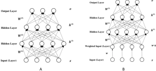
Deep Feature Selection (Yifeng Li, 2015) [17] is a network architecture between input layer and first hidden layer. In order to demonstrate the compact of every feature in input space, they proposed an one-to-one element-wise product layer. The architecture shows in Figure 1, and the additional regularization loss formats in Equation 1.
𝑦$%&' = 𝑓 𝑥 ⊙ 𝑤 𝜃) 𝑥, 𝑤 ∈ 𝑅'
min4 𝑓 𝜃 = 𝑙 𝑦$%&', 𝑦6%7& + 𝛼 𝑊 ;+ 𝛽 𝑤 = (1)
𝑊 ; denotes the common L2 regularization loss for parameters of network, 𝑤 = denotes the regularization loss on additional one-to-one layer. They use the L1 to make 𝑤= sparse to achieve the goal, which is feature selection. In the original paper, they rank the features by magnitude of corresponded weight in 𝑤.
A B
Figure 1: The Deep Feature Selection (DFS) – model architecture.
(A) : The fully-connective network, with 2 hidden layer. (B) The DFS with 2 hidden layer and one-to-one element-wise product layer. [17]
3.2 SelectNet
To achieve the sparser structure, we first introduce a new hyper-parameter 𝑝, where 0 < 𝑝 ≤ 1, to replace the regularization norm over 𝑤.
𝑦$%&' = 𝑓 𝑥 ⊙ 𝑤 𝜃) 𝑥, 𝑤 ∈ 𝑅'
min4 𝑓 𝜃 = 𝑙(𝑦$%&', 𝑦6%7&) + 𝛼 𝑊 ; + 𝛽 𝑤 $ (2) Moreover, we use the ratio over values of 𝑤 to rank features.
𝑤%F6GHI = 𝑤G 𝑤J
'J
𝑦$%&' = 𝑓 𝑥 ⊙ 𝑤%F6GH 𝜃) 𝑥, 𝑤 ∈ 𝑅'
min4 𝑓 𝜃 = 𝑙(𝑦$%&', 𝑦6%7&) + 𝛼 𝑊 ; + 𝛽 𝑤 $ (3)
After network converges, weight of the one-to-one layer can show what features are actually in use. With strong regularization loss, the network tends to fit the problem with the less features. In the following experiments, we also add a hyper-parameter calls ratio threshold, initialized by L.='. It’s a threshold activation function to one-to- one layer. Since the ratio values lower than threshold will be set zero, the feature could be seen as unnecessary feature for network.
3.3 Improvement
The DFS faces 2 major shortcomings in feature selection and computing.
l Weights of 𝑤 converge toward an extreme small value.
l Accuracy dropping, because of covariate shift, and floating point computing problem in extreme small value.
In formula (1), every 𝑤G is supposed to be small. It is hard to tell whether a feature is in use when even the greatest weight is lower than 10MN. Moreover, those weights may be recovered by the hidden layer with large weights.
Figure 2: The SelectNet – model architecture.
We calculated ratio in one-to-one layer.
The second is about the performance dropping, we notice that after applying DFS on original network, the network perform worse. Based on this observation, we assume the reason is caused by floating computation problem and covariate shift.
When the inputs go through an extreme small value, they may still be recovered by hidden layer with large weights. The authors of DFS introduced L2 regularization on
𝑊 ; to restrain this behavior, but covariate shift still remains the problem.
Our method use ratio to control the gate weight, so its convergence is bounded within [1,'=] in practical, which prevents the covariate shift. It can also easily tell which features are actually used by introducing the ratio threshold. By the thumb rule, we set ratio threshold as 10MQ in all experiments
Chapter 4 Experiments
In this section, we present the performance in 3 methods and 4 datasets.
Three methods are listed below.
l Naive DNN, only with hyper-parameter 𝛼 to control regularization loss of kernel weight matrix.
𝐿𝑜𝑠𝑠 = 𝐿𝑜𝑠𝑠 𝑦, 𝑦 + 𝛼 𝜃 ;; l Deep Feature Selection(DFS), the method from [6].
𝐿𝑜𝑠𝑠 = 𝐿𝑜𝑠𝑠 𝑦, 𝑦 + 𝛼 𝜃 ;;+ 𝛽 𝑤 = l SelectNet, our proposed method.
𝐿𝑜𝑠𝑠 = 𝐿𝑜𝑠𝑠 𝑦, 𝑦 + 𝛼 𝜃 ;;+ 𝛽 𝑤%F6GH $, 0 < 𝑝 ≤ 1 Four datasets are listed below.
1. Synthesized-easy 2. Synthesized-hard 3. MNIST
4. Dengue fever binary classification
The first two datasets are synthesized, and we use the easy one to test the ability of feature selection. Then, we use the 2nd one to show the importance of denoising.
The third one is MNIST, a released image dataset for many benchmarks. Because images are more interpretable than numeric features, we use it to show the correctness in comprehensible dataset. At last, we apply this method to a real world medical binary classification problem.
All the experiment results have been smoothed, we implemented the same logic with Tensorboard smooth variable as 0.8.
4.1 Model Selection
To select the best hyper-parameters, we used the following rule:
𝑝 ∈ {0.25, 0.5, 0.75, 1.0}
𝛼 ∈ {0.1}
𝛽 ∈ {1, 10, 100, 1000}
𝛾 ∈ 0
In every dataset, we train 3 times, ensuring to avoid the sampling bias. To
demonstrate the ability of feature selection, the sparest feature group will be selected by top 3 at accuracy.
4.2 Synthesized-easy
It’s a 2D binary classification dataset with 6 extra noised features, shows as Figure 3.
It contains 3 types of noised feature:
redundant feature, random distribution and random permutation. Also, we add 10%
missing with mean value for each feature to increase the complexity of this dataset.
We denote 𝑈 𝑎, 𝑏 as Uniform
distribution within 𝑎, 𝑏 . 𝑃𝑒𝑟𝑚𝑢𝑡𝑎𝑡𝑖𝑜𝑛 𝑥 as random permutation without association
with label. The reason why we choose random permutation is based on [18] because the noised feature may share some similar characteristic with the original feature.
Figure. 3 Synthesized-easy
0.02𝑥=N− 0.5𝑥=;+ 0.8𝑥;+ 12 separate hyper-plane of synthesized-easy dataset
The definition of all features shows as following:
𝑥= ∼ 𝑈 𝑎, 𝑏 | 𝑎 = −50, 𝑏 = 75 𝑥; ∼ 𝑈 𝑎, 𝑏 | 𝑎 = −50, 𝑏 = 75
𝑥N = −0.5𝑥;
𝑥i ∼ 𝑈 𝑎, 𝑏 | 𝑎 = −50, 𝑏 = 75 𝑥Q ∼ 𝑁 𝜇, 𝜎; | 𝜇 = 12.5, 𝜎 = 10
𝑥m = 𝑃𝑒𝑟𝑚𝑢𝑡𝑎𝑡𝑖𝑜𝑛 𝑥= 𝑥n = 𝑃𝑒𝑟𝑚𝑢𝑡𝑎𝑡𝑖𝑜𝑛 𝑥=; 𝑥o = 𝑃𝑒𝑟 𝑚𝑢𝑡𝑎𝑡𝑖𝑜𝑛 𝑥; 𝑦 = 0.02𝑥=N− 0.5𝑥=;+ 0.8𝑥;+ 12
In this experiment, all three results, including the naive DNN, use fully
connected network with 3 hidden-layer, hidden dimension as 16, as their downstream model. Table.1 lists top 3 hyper-parameter sets for each method. Figure. 4 shows the accuracy, and Figure. 5 represents the result of feature selection corresponding to SelectNet and DFS.
Based on the results, both SelectNet and DFS find the key feature with slight difference, passing the noise test as well. In contrast to DFS, SelectNet filters out the redundant feature −0.5𝑥;.
In conclusion, both methods work in this dataset, though DFS shows the
drawback of dropping accuracy. The noise didn’t make significant effect on the naive FCN. Most likely, this dataset is too easy to show the benefit of finding the key
feature. Therefore, in next section we design an advanced dataset based on this one, to demonstrate the importance of fitting on noised features.
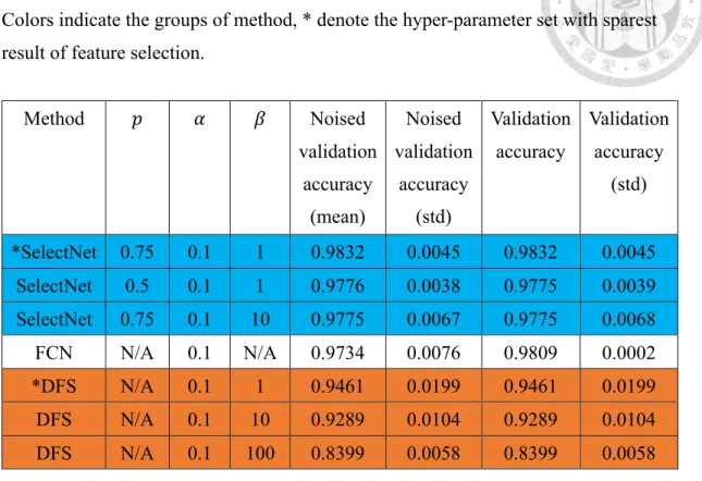
Table 1: Performance in Synthesized Easy dataset.
Colors indicate the groups of method, * denote the hyper-parameter set with sparest result of feature selection.
Method 𝑝 𝛼 𝛽 Noised
validation accuracy
(mean)
Noised validation
accuracy (std)
Validation accuracy
Validation accuracy
(std)
*SelectNet 0.75 0.1 1 0.9832 0.0045 0.9832 0.0045 SelectNet 0.5 0.1 1 0.9776 0.0038 0.9775 0.0039 SelectNet 0.75 0.1 10 0.9775 0.0067 0.9775 0.0068
FCN N/A 0.1 N/A 0.9734 0.0076 0.9809 0.0002
*DFS N/A 0.1 1 0.9461 0.0199 0.9461 0.0199
DFS N/A 0.1 10 0.9289 0.0104 0.9289 0.0104
DFS N/A 0.1 100 0.8399 0.0058 0.8399 0.0058
Figure. 4: Accuracy of training/validation set in Synthesize-easy.
Figure. 5: Feature selection in Synthesized-easy.
(A) The w value of DFS. (B) The w values of SelectNet. (C) The w ratio of DFS, 2 features were selected. (D) The ratio of SelectNet, 2 features were selected. Except the top 2 features, the rest all reach the lower bound. Which all were set to zero.
A B
C D
4.3 Synthesized-hard
To emphasize the benefit of feature selection, we design an advanced dataset, altered from previous one. In this experiment, SelectNet shows the better performance in accuracy and feature selection.
It’s also a 2D binary classification dataset with 6 extra noised features same as previous one, added non-linear transform, shows as Figure 6.
We only add 5% missing noise to each feature in this dataset, in contrast to adding 10% the easier one.
Table.2 lists top 3 hyper-parameter sets for each method. Figure. 7 shows the accuracy, and Figure. 8 represents the result of feature
selection corresponding to SelectNet and DFS.
In this experiment, the naive FCN fits on the wrong features, so the accuracy drops dramatically. On the other hand, both DFS and SelectNet fit on the key features, but the drawback of DFS we mention in Section 3 shows up. When feature passes through an extreme small weight, it raises the hardness of converge. That may be the reason accuracy drops.
Figure. 6 Non-linear separate hyper-plane of synthesized-hard dataset
Table 2: Performance in Synthesized Hard.
Colors indicate the groups of method, * denote the hyper-parameter set with sparest result of feature selection.
Method 𝑝 𝛼 𝛽 Noised
validation accuracy
(mean)
Noised validation
accuracy (std)
Validation accuracy
Validation accuracy
(std)
*SelectNet 0.5 0.1 10 0.9137 0.0114 0.9137 0.0114
DFS N/A 0.1 1 0.8938 0.0027 0.908 0.0048
SelectNet 0.25 0.1 1 0.8884 0.0229 0.8884 0.0229 SelectNet 0.75 0.1 100 0.8753 0.0052 0.8753 0.0052
*DFS N/A 0.1 10 0.8602 0.0238 0.8602 0.0238
FCN N/A 0.1 N/A 0.6144 0.0322 0.7755 0.0357
DFS N/A 0.1 100 0.5491 0.0568 0.5491 0.0568
Figure.7: Accuracy of training/validation set in Synthesized-hard
Figure.8: Feature selection in Synthesized-hard
(A) The w value of DFS. (B) The w values of SelectNet. (C) The w ratio of DFS, 3 features were selected. (D) The ratio of SelectNet, 2 features were selected. Except the top 2 features, the rest all reach the lower bound. Which all were set to zero.
A B
D C
4.4 MNIST
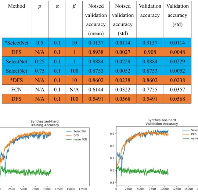
In this multi-class image classification dataset, MNIST, we examine SelectNet to see whether it can still fit on the key feature in real-world data. For this purpose, we add noise on the border, where the pixels are unnecessary for naked eyes to distinguish digits. Additionally, we resize to 10x10x1 grayscale image and use the CNN and Max pooling as downstream model.
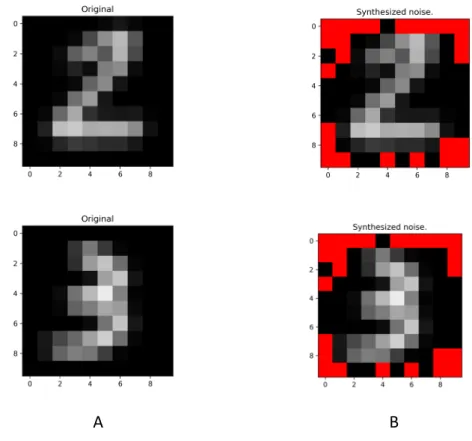
Figure 9 shows the coverage of noise. Figure 10 shows the benefit from feature
Figure.9: (A) The original image with label 2 in 10x10 pixels. (B) The noised image covered with red pixels, but the contour is still clear. The Noised validation accuracy shows the performance which model trained on images likes (A), then tested in (B).
A B
selection, emphasizing the ability to defense noise from unnecessary features. If the model can fit on the key features, the central pixels, it should avoid the noise on the border. Figure 10 shows the pixel coverage that DFS and SelectNet actually used.
Both DFS and SelectNet generated similar result, and the exposed region is sufficient to be differentiated by human vision. As the result, we conclude that the models find a subset of features to do this classification. In contrast to DFS, SelectNet ends up with some zero weights in one-to-one layer, so it’s clear to demonstrate unnecessary features, which is also the improvement we mentioned in Section 3. Overall, the SelectNet keeps the performance in validation set, and avoids the effect from noise on
Figure.10: (A) The original image with label 2 in 10x10 pixels. (B) The noised image covered with red pixels, but the contour is still clear. The Noised validation accuracy shows the performance which model trained on images likes (A), then tested in (B).
A B
unnecessary features. Table 3 shows the top 3 hyper-parameter sets of models.
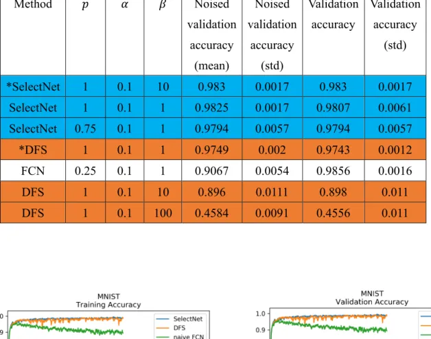
Table 3: Performance in MNIST dataset.
Colors indicate the groups of method, * denote the hyper-parameter set with sparest result of feature selection.
Method 𝑝 𝛼 𝛽 Noised
validation accuracy
(mean)
Noised validation
accuracy (std)
Validation accuracy
Validation accuracy
(std)
*SelectNet 1 0.1 10 0.983 0.0017 0.983 0.0017
SelectNet 1 0.1 1 0.9825 0.0017 0.9807 0.0061
SelectNet 0.75 0.1 1 0.9794 0.0057 0.9794 0.0057
*DFS 1 0.1 1 0.9749 0.002 0.9743 0.0012
FCN 0.25 0.1 1 0.9067 0.0054 0.9856 0.0016
DFS 1 0.1 10 0.896 0.0111 0.898 0.011
DFS 1 0.1 100 0.4584 0.0091 0.4556 0.011
Figure.11: Accuracy of training/validation set in MNIST
4.5 Dengue Fever binary classification
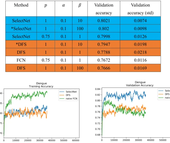
In this experiment, we discuss our first assumption, whether the feature selection benefit models in highly redundant input space. This dataset contains 63 features in total. However, our expert filter out 11 key features, and gain higher performance than training with 63 features. Under this premise, we expect SelectNet should improve the accuracy, and show similar result with experts.
Table 4: Performance in Dengue Fever dataset.
Colors indicate the groups of method, * denote the hyper-parameter set with sparest result of feature selection.
Method 𝑝 𝛼 𝛽 Validation
accuracy
Validation accuracy (std)
SelectNet 1 0.1 10 0.8021 0.0074
*SelectNet 1 0.1 100 0.802 0.0098
SelectNet 0.75 0.1 1 0.7998 0.0126
*DFS 1 0.1 10 0.7947 0.0198
DFS 1 0.1 1 0.7788 0.0218
FCN 0.75 0.1 1 0.7672 0.0116
DFS 1 0.1 100 0.7666 0.0169
Figure.12: Accuracy of training/validation set in Dengue Fever.
A B
Figure.13: (A) The w value of DFS. (B) The w values of SelectNet. (C) The w ratio of DFS, 6 features were
selected. (D) The ratio of SelectNet, 26features were selected. Except the top 6 features, the rest all reach the lower bound. Which all were set to zero.
A
C D
B
Chapter 5 Conclusion and Future Works
In this work, we presented the SelectNet, a regularization layer learning structured sparsity in input space, showing the sufficient subset of features.
For classification task, the SelectNet performed better than naive FCN/CNN at noise data/images without harming the accuracy in default validation set. In feature
selection aspect, SelectNet can directly show what features that network actually used.
A further study with more focus on correctness of feature selection should be carefully examined. More experiments in human comprehensible data will increase confidence of this method.
Overall, SelectNet is more stable than DFS in accuracy, more interpretable than naive network.
References
[1] Ashish Vaswani, Noam Shazeer, Niki Parmar, Jakob Uszkoreit, Llion Jones, Aidan N. Gomez, Lukasz Kaiser, Illia Polosukhin. 2017. Attention Is All You Need. In NIPS [2] Čehovin, Luka & Bosnic, Zoran. 2010. Empirical evaluation of feature selection
methods in classification. Intell. Data Anal.. 14. 265-281. 10.3233/IDA-2010-0421.
[3] Devlin, J., Chang, M., Lee, K., & Toutanova, K. 2018. BERT: Pre-training of
Deep Bidirectional Transformers for Language Understanding.
ArXiv,abs/1810.04805.
[4] Gui, Jie & Sun, Zhenjun & Ji, Shuiwang & Tao, Dacheng & Tan, Tieniu. 2016.
Feature Selection Based on Structured Sparsity: A Comprehensive Study. In IEEE
Transactions on Neural Networks and Learning Systems. 1-18.10.1109/TNNLS.2016.2551724.
[5] Jundong Li, Kewei Cheng, Suhang Wang, Fred Morstatter, Robert P. Trevino, Jiliang Tang, and Huan Liu. 2017. Feature selection: A data perspective. In ACM Computing Surveys
[6] Ji Zhu, Saharon Rosset, Robert Tibshirani, and Trevor J Hastie. 2004. 1-norm
support vector machines. In NIPS. 49–56.
[7] Kelvin Xu, Jimmy Ba, Ryan Kiros, Kyunghyun Cho, Aaron Courville, Ruslan Salakhutdinov, Richard Zemel, Yoshua Bengio. 2015. Show, Attend, and Tell: Neural
image caption generation with visual attention. In ICML
[8] Liping Wang, Songcan Chen, Yuanping Wang. 2014. Comput. Optim. Appl., vol.
58, no. 2, pp. 409–421
[9] Lin, Min, Qiang Chen and Shuicheng Yan. 2013. Network In Network. CoRR, abs/1312.4400
[10] Matthew D Zeiler, Rob Fergus. 2013. Visualizing and Understanding
Convolutional Networks. In EVCC.
[11] Miao Zhang, Chris Ding, Ya Zhang, Feiping Nie. 2014. Feature Selection at the
discrete limit. In AAAI 1355–1361.
[12] Quanquan Gu, Zhenhui Li, Jiawei Han. 2011. Generalized Fisher score for
feaure selection. In Proc. 27th Conf. Uncertainty Artif. Intell., pp. 266–273.
[13] Richard O Duda, Peter E Hart, and David G Stork. 2001. Pattern Classification,
2nd ed. Hoboken, NJ, USA: Wiley.
[14] Rudy Setiono. 1997. A penalty-function approach for pruning feedforward
neural networks. In Neural Comput. 185-204.
[15] Rudy Setiono and Huan Liu. 1997. Neural-network feature selector. in IEEE Transactions on Neural Networks, vol. 8, no. 3, pp. 654-662
[16] Thomas M. Cover, Joy A. Thomas. 2006. Elements of Information Theory. 2nd ed. New York, NY, USA: Wiley.
[17] Yifeng Li, Chih-Yu Chen, and Wyeth W Wasserman. 2015. Deep feature
selection: theory and application to identify enhancers and promoters. In RECOMB.
205–217.
[18] Yang Young Lu, Yingying Fan, Jinchi Lv, William Stafford Noble. 2018.
DeepPINK: reproducible feature selection in deep neural networks. In NIPS.
[19] Zhouhan Lin, Minwei Feng, Cicero Nogueira dos Santos, Mo Yu, Bing Xiang, Bowen Zhou, Yoshua Bengio. 2017, A structured Self-attentive sentence embedding.
In ICLR.