國立臺灣大學管理學院資訊管理學研究所 碩士論文
Graduate Institute of Information Management College of Management
National Taiwan University Master Thesis
點集合影片資料庫中封閉性樣式之資料探勘 Mining Closed Patterns in Pointset Video Databases
賴奕伃 Lai, Yi-Yu
指導教授:李瑞庭 博士 Advisor: Anthony J. T. Lee, Ph.D.
中華民國 97 年 7 月
July, 2008
點集合影片資料庫中封閉性樣式之資料探勘 Mining Closed Patterns in Pointset Video Databases
本論文係提交國立台灣大學 資訊管理學研究所作為完成碩士
學位所需條件之一部份
研究生:賴奕伃 撰 民國九十七年七月
謝辭
本篇論文得以順利完成,首先我要感謝我的指導教授李瑞庭老師,他認真嚴 謹的研究及教學態度、親切有耐心的指導以及他謙遜包容的待人處事,在我的研 究生涯給了我很大的幫助和一個值得學習的榜樣,真的非常感謝老師。在研究以 外,老師也常與我們分享生活中的點滴,給予我許多啟發,真的很高興有這個機 會能夠加入老師的實驗室跟隨老師做研究。
再來我要感謝口試委員陳良華老師、沈錳坤老師細心的提問並提出許多寶貴 的意見,讓本篇論文更加的完整。也感謝所上老師的認真教學,讓我在資管所學 到了許多有用的知識和做人處事的道理。
感謝實驗室的同學們:春宏、柏吟、韻茹、韋廷、明志,在我的研究和生活 上幫助我非常多;好相處的學弟妹:巽評、榮泰、惠萍、景瑋,不僅在我的口試 當天幫忙、平日也給了我很多歡笑和感動;博班的學長姊:怡安、惠雯、文光,
在研究上給了我許多建議和鼓勵。也感謝已經畢業的學長姊,在碩一時對我的關
懷和照顧。非常榮幸能加入Tony Lab,和大家相處的點滴會成為我難忘的回憶。
感謝所上的好朋友:子超、孜謙、奐廷、家禎、至浩、偉倫、文振,陪伴我 度過充滿歡笑及淚水的研究所生涯,也給予我許多的鼓勵和幫助。感謝我高中的
摯友之珺和宜薇、大學的802 室友們不論何時一直給我最大的鼓勵和支持。
最後要感謝我的家人,爹、娘、大哥一直以來對我的支持,照顧我的日常生 活、讓我無後顧之憂地念研究所,非常謝謝你們,沒有你們就沒有今天的我。要 感謝的人還有很多很多,在此,謹以此論文獻給我最愛的親人、師長和朋友們。
賴奕伃 謹識 于台大資訊管理學研究所 中華民國九十七年七月
論文摘要
論文題目:點集合影片資料庫中封閉性樣式之資料探勘
作者:賴奕伃 九十七年七月 指導教授:李瑞庭 博士
隨著多媒體影像技術的蓬勃發展,多媒體資料量快速地遽增,如何從龐大的 多媒體資料中找到有意義的資訊和特性已成為熱門的研究議題。我們可以將影片 中發生的一個事件視為一個連續的點集合,而找到影片資料庫中由點集合所構成 的封閉性樣式,則可以表達出影片中發生該事件的特性。因此,在本論文中,我 們提出一個有效率的探勘演算法「CVP」來探勘出影片資料庫中的封閉性樣式。
我們所提出的演算法主要先利用兩種資料結構儲存頻繁樣式的資訊,以深度優先 搜尋的方式先對空間維度、再對時間維度產生出可能的頻繁樣式,最後再利用我 們所提出的方法來修剪不符合或不必要的樣式以及判斷其封閉性。我們的演算法 利用投影資料庫去產生可能的樣式和進行修剪,並不需要重複地搜尋整個影片資 料庫,因此效率能夠得到明顯的改善。在人造及真實資料庫的實驗結果中顯示我
們所提出的方法較改良式Apriori 的方法來得更有效率。
關鍵詞:資料探勘、點集合影片資料庫、封閉性樣式、頻繁樣式
THESIS ABSTRACT
Mining Closed Patterns in Pointset Video Databases
By Yi-Yu Lai
DEPARTMENT OF INFORMATION MANAGEMENT NATIONAL TAIWAN UNIVERSITY
July, 2008
ADVISOR: Anthony J. T. Lee, Ph.D.
Nowadays, the number of multimedia datasets is increasing rapidly. Thus, mining implicit and meaningful patterns from multimedia databases has attracted more and more attention in recent years. The event object can be viewed as a sequence of pointsets in a video. Mining closed patterns in pointset video databases can help us understand the pattern of an event in video databases. In this thesis, we first devise two data structures, called rplist and CV-tree, to store the information of frequent video patterns. Next, we propose a novel algorithm, called CVP, to mine frequent closed patterns from a video database in a depth-first search (DFS) manner.
Our proposed algorithm consists of two phases. We first grow frequent video patterns in the spatial dimension and then grow them in the temporal dimension. To efficiently mine frequent closed patterns, we develop several pruning strategies to prune non-closed patterns. The CVP algorithm can localize the candidate generation, pattern join, and support counting in a small amount of rplists. Therefore, it can efficiently mine frequent closed patterns in a video database. The experiment results show that our proposed method outperforms modified Apriori algorithm in synthetic data and real data.
Keywords: data mining, pointset video database, closed pattern, frequent pattern
i
Table of Contents
Table of Contents ... i
List of Figures ... ii
List of Tables ... iii
Chapter 1 Introduction ... 4
Chapter 2 Preliminaries and Problem Definitions ... 8
Chapter 3 Our Proposed Method ... 12
3.1 Rplist and CV-tree ... 12
3.2 Pattern generation ... 14
3.3 Closure checking and pruning strategies ... 21
3.4 The CVP algorithm ... 25
3.5 An example ... 29
Chapter 4 Performance Evaluation ... 33
4.1 Synthetic datasets ... 34
4.2 Performance evaluation on synthetic datasets ... 34
4.3 Performance evaluation on real datasets ... 38
Chapter 5 Conclusions and Future work ... 41
References ... 42
ii
List of Figures
Figure 1. Three frames of video v1 with frame size of 3×3 ... 8
Figure 2. An example video database ... 11
Figure 3. Candidate 2-spatterns with frame size of 3×3 ... 13
Figure 4. The CV-tree containing frequent 2-spatterns ... 14
Figure 5. Joining two spatterns ... 15
Figure 6. Growing patterns in the spatial and temporal dimensions ... 19
Figure 7. The growing representation of the CV-tree ... 20
Figure 8. Four pruning strategies ... 24
Figure 9. Closure checking in vpattern pruning ... 25
Figure 10. The CVP algorithm ... 26
Figure 11. The CVPGrowth function ... 27
Figure 12. The GrowSNode function ... 28
Figure 13. The GrowTNode function ... 28
Figure 14. Growing closed vpatterns ... 30
Figure 15. Closed vpatterns in the closed pattern set... 32
Figure 16. Runtime versus minimum support ... 35
Figure 17. Runtime versus number of videos ... 35
Figure 18. Runtime versus maximum time span ... 36
Figure 19. Number of closed patterns versus maximum time span ... 36
Figure 20. Runtime versus number of frames ... 37
Figure 21. Number of closed patterns versus number of frames ... 38
Figure 22. A real video dataset ... 39
Figure 23. A closed pattern mined ... 40
iii
List of Tables
Table 1. Parameters used to generate synthetic data ... 34 Table 2. Parameters used in the real dataset ... 39 Table 3. Experiment results of a throwing-ball dataset ... 40
4
Chapter 1 Introduction
With advances in information technologies, a large amount of videos have been collected into video databases. Thus, the approaches of mining useful patterns from video databases have been attracted more and more attention in recent years. If we known what patterns often happen in the videos, we will know what situations often occur and to what we should pay attention. For example, we put a video camera on corridor in a hospital to collect how the patients walk. Many videos will be collected into a video database. By mining frequent patterns in such a database, we could know the pattern of normal walk of patients and abnormal ones, like patients falling down to the ground. If a patient falls down to the ground, an alarm will be raised to notify the workers in the first-aid station. If we can know the pattern of patients falling down in the video database, it could help a monitoring system to detect this event automatically, and inform the first-aid station immediately. We can also detect other kinds of movement patterns of human beings to achieve some purpose of security protection. For instance, if we can obtain the patterns of the action of throwing, it is helpful to avoid some violent behaviors such as throwing a grenade or other weapons.
A pattern is frequent if it satisfies the user-specified minimum support. There are many kinds of frequent patterns, including itemsets, subsequences, substructures, etc. A frequently-occurring subsequence, such as the pattern that customers tend to purchase first a PC, followed by a digital camera, and then a memory card, is also called a sequential pattern. Sequential pattern mining, which discovers frequent subsequences in a sequence database, is a critical data mining problem with board applications, including the analyses of customer purchase behavior, Web access patterns, scientific experiments, DNA sequences, and so on.
Many sequential mining methods have been proposed. Agrawal et al. [1]
5
proposed an Apriori method, which adopts a generate-and-test approach to mine sequential patterns. The major approaches of mining a complete set of sequential patterns include SPAM [2], GSP [16], SPADE [20], GO-SPADE [10] and PrefixSpan [14]. GSP [16] uses the downward-closure property of sequential patterns and adopts the candidate generate-and-test approach to mine sequential patterns. SPADE [20] and GO-SPADE [10] devises a divide-and-conquer strategy to implement the sequential patterns mining with a vertical data format. SPAM [2] exploits a vertical bitmap structure to count supports efficiently. However, the Apriori-based methods would generate many redundant candidates and require multiple database scans. Thus, Han et al. [4] designed the FP-growth method to mine frequent itemsets without candidate generation. Han et al. [5] proposed the FreeSpan method, which recursively projects a sequential database into projected databases, and generates frequent sequential patterns from these projected databases. PrefixSpan [14] mines the complete set of patterns but greatly reduces the efforts of candidate subsequence generation.
Moreover, using prefix-projection can substantially reduces the size of projected databases and leads to mining the patterns efficiently.
Many methods have been proposed to mine frequent subgraphs. Inokuchi et al.
[7] proposed an AGM method to represent a graph as an “adjacency matrix” and mine them with an Apriori-based approach. Kuramochi et al. [9] presented an FSG method based on the Apriori algorithm, which uses a sparse graph representation to minimize storage space and computation time and has various optimization techniques for candidate generations. Yan et al. [19] developed a depth-first search algorithm, gSpan, to mine frequent subgraphs without candidate generations, where the DFS lexicographic order and minimum DFS code are used to represent a graph. Huan et al.
[6] designed a candidate subgraph enumeration scheme, called FFSM, to mine frequent subgraphs. Wang et al. [8] proposed a method that eliminates some vertices in a path of a graph which can keep the topology structures in the graph and also reduce the search space to increase the mining efficiency.
6
Instead of mining all frequent itemsets, Pasquier et al. [12] introduced a new concept to mine the frequent closed itemsets. A frequent itemset is closed if there does not exist any super-itemset with the same support. However, the number of closed itemsets must be not greater than that of frequent itemsets in the database and frequent closed itemsets mined can be used to generate a complete set of frequent itemsets [12].
Generally speaking, mining closed itemsets is more efficiently than mining all frequent itemsets [12]. A-CLOSE [12] exploits the Apriori property to find closed itemsets. CLOSET [13] and CLOSET+ [18] uses the FP-tree as a compact data structure and mines frequent closed itemsets by projected databases. CHARM [21]
uses an itemset-tidset search tree and applies a diffset technique to increase its performance. DCI_CLOSED [11] can detect and discard the duplicate closed itemsets without the need of keeping the closed itemsets mined in main memory. Singh et al.
[15] proposed the CloseMiner algorithm to mine closed itemsets where they considered the frequent closed itemset mining problem as the problem of clustering the complete set of itemsets with closed tidsets. Uno et al. [17] developed the LCM algorithm, which organizes the closed itemsets into a tree structure and mines them in a depth-first search manner. Cheng et al. [3] proposed an algorithm to mine δ-tolerance frequent closed itemsets (δ-TCFIs) in order to reduce the number of closed itemsets.
However, the itemset mining methods proposed cannot use to mine the patterns in video databases. The sequential mining methods do not consider the spatial attribute in the video patterns. The graph mining methods cannot be used to mine the patterns in video databases because they do not consider the temporal attribute.
Therefore, the itemset mining, sequential mining and graph mining methods are not suitable to mine frequent closed patterns in video databases.
Therefore, in this thesis, we first devise two data structures, called rplist and CV-tree, to store the information of frequent video patterns. Next, we propose a novel algorithm, called CVP, to mine frequent closed patterns from a video database in a
7
depth-first search (DFS) manner. Our proposed algorithm consists of two phases. We first grow frequent video patterns in the spatial dimension and then grow them in the temporal dimension. To efficiently mine frequent closed patterns, we develop several pruning strategies to prune non-closed patterns. By exploiting the CV-tree and rplists to store the information of frequent video patterns, the CVP algorithm can localize the candidate generation, pattern join, and support counting in a small amount of rplists.
Therefore, it can efficiently mine frequent closed patterns in a video database.
The contributions of this thesis are summarized as follows: (1) We first devise two data structures, called rplist and CV-tree, to store the information of frequent video patterns. (2) We propose a novel algorithm, called CVP, to mine frequent closed patterns from a video database in a depth-first search (DFS) manner. (3) To efficiently mine frequent closed patterns, we develop several pruning strategies to prune non-closed patterns. (4) By exploiting the CV-tree and rplists to store the information of frequent video patterns, the CVP algorithm can localize the candidate generation, pattern join, and support counting in a small amount of rplists. (5) The experimental results show that our proposed algorithm is efficient and scalable, and outperforms the modified Apriori algorithm.
The rest of this thesis is organized as follows. Chapter 2 illustrates the preliminary concepts and problem definitions. Chapter 3 describes our proposed algorithm. Chapter 4 shows the experimental setup and performance evaluation.
Finally, the conclusions and future work are discussed in Chapter 5.
8
Chapter 2 Preliminaries and Problem Definitions
In this chapter, we will first describe the preliminary concepts and then define some terms used in this thesis.
Consider a video database D={v1,v2,…,vn} contains n videos, n>1. These videos are preprocessed into several frames, where each frame contains one object and is converted to a bitmap (or binary) image in a two-dimensional space, and the frame size is g×g, g>2. Let vi,j indicate the jth frame of video vi. vi,j is represented by a bitmap. For example, Figure1 illustrates three frames of video v1 with frame size of 3×3. We can use 9 bits to represent the contents of each frame and the frame v1,1 is denoted as (010 010 010). That is, we list the contents in bits row by row.
Figure 1. Three frames of video v1 with frame size of 3×3
Definition 1. A spatial pattern (spattern for short) is defined as (a1a2…ag2), where ai
= 0 or 1, i = 1,2,…,g2. The length of an spattern is defined as the number of 1-bits in the spattern. An spattern of length l is called an l-spattern. For example, the first frame of the video shown in Figure 1 can be denoted as (010 010 010), which is a 3-spattern.
Definition 2. A pixel in a video is denoted by (x,y,t), where (x,y) is the coordinate of the pixel in frame t. A pixelset contains a set of pixels. For example, the first frame of the video shown in Figure 1 can be denoted as {(2,1,1), (2,2,1), (2,3,1)}.
Definition 3. Given two spatterns S=(a1a2…ag2) and S’=(b1b2…bg2), where 1<i<g2. If there exists an integer j such that if bi+j=1 when aj=1, j=k,k+1, …, l, we can say that S is contained by S’, denoted as S⊆S’, where ak is the first 1-bit and al is the last 1-bit in S. We can also say that S is a sub-spattern of S’, or S’ is a super-spattern of S.
v1,3
v1,2
v1,1
v1
9
Moreover, an spattern S is contained by a video if there exists a frame containing S in the video. For example, S=(110 100 000) is a sub-spattern of S’=(011 110 000).
Definition 4. If an spattern S is contained by the tth frame of video v, the reference point of S is denoted as (x,y,t,v), where (x,y) is the coordinate of the uppermost and leftmost pixel of S appearing in frame t. For example, the reference point of 3-spattern (010 010 010) appears in the first frame of video 1 shown in Figure 1. Thus, its reference point can be denoted as (2,1,1,1). The reference points of 2-spattern (100 100 000) are (2,1,1,1) and (2,2,1,1).
Definition 5. The support of an spattern S, denoted as sup(S), is defined as the number of videos containing S in the database. S is frequent if sup(S) is not less than a user-specified minimum support threshold, minsup.
Definition 6. A frequent spattern S is closed if there does not exist any super-spattern of S with the same support.
Definition 7. The projected database prj(S) of an spattern S contains a set of reference points of the frames containing S in the database. The prj(S) of 2-spattern S=(100 100 000) in video v1 shown in Figure 1 is {(2,1,1,1), (2,2,1,1), (2,1,2,1), (2,2,2,1), (2,1,3,1), (2,2,3,1)}. It means that the 2-spattern appears at (2,1) and (2,2) in the first frame, at (2,1) and (2,2) in the second frame, and (2,1) and (2,2) in the third frame of v1.
A video pattern is formed by a sequence of spatterns. To represent a video pattern flexibly, we introduce a time span between two adjacent spatterns in the video pattern, where a time span is denoted as [t1, t2], t1 and t2 are positive integers, t1<t2. It means that the distance between both adjacent spatterns can be from t1 to t2 frames.
Definition 8. A video pattern (or vpattern for short) is defined as S1[t11, t12]S2[t21, t22]S3…Sk, where Si is an spattern, i = 1, 2,…, k, and the time span between Sj and Sj+1
is [tj1, tj2]. The length of a vpattern is defined as the number of spatterns in it. A
10
vpattern of length k is called a k-vpattern. A 1-vpattern, which is also an spattern, does not have any time span. That is, an spattern is a special case of vpatterns. For example, the 3-vpattern in video v1 shown in Figure 1 is denoted as (010 010 010)[1,1](011 010 010)[1,1](011 110 010).
Since a vpattern can span many frames, discovering all such vpatterns would require a lot of resources, but a user may only be interested in vpatterns that span a certain number of frames. Therefore, to avoid wasting resources by mining unwanted vpatterns, we introduce a parameter called maxinterval. When mining vpatterns in a video database, we only find the vpatterns where the time span between any two adjacent spatterns in the vpatterns is not greater than maxinterval.
Definition 9. A vpattern V=S1[t11, t12]S2[t21, t22]S3…Sk is contained by another vpattern V’=S’1[t’11, t’12]S’2[t’21, t’22]S’3…S’l if we can find k spatterns S’j1, S’j2,…, S’jk in V’ such that Si is contained by S’ji and [ti1, ti2] is equal to [tji1, tji2], where 1<i<k, and k<l. We can also say that V is a subpattern of V’, or V’ is a super-pattern of V, denoted as V⊆V’. For example, V=(100 110 100)[1,3](010 111 010)[1,3](001 011 001) is contained by V’=(111 111 100)[1,3](011 111 010)[1,3](001 011 001).
Definition 10. A vpattern V=S1[t11, t12]S2[t21, t22]S3…Sk is contained by a video if we can find k frames, f1, f2,…, fk, in the video so that fi contains Si, and the time span between fj and fj+1 is within [tj1, tj2], where i=1,2,…, k and j=1,2,…, k-1.
Definition 11. The support of a vpattern V, denoted as sup(V), is defined as the number of videos containing V in the database. V is frequent if sup(V) is not less than a user-specified minimum support threshold, minsup.
Definition 12. A frequent vpattern V is closed if there does not exist any super-pattern of V with the same support. Note that if S1[1,2]S2 and S1[1,3]S2 have the same support, S1[1,3]S2 is not closed since [1,3] contains [1,2] and S1[1,3]S2 is less expressive.
11
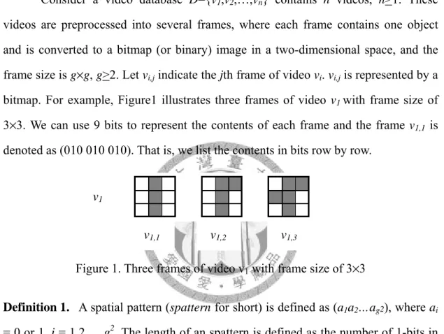
Definition 13. The projected database prj(v) of a vpattern v is donoted as {(t1,v1), (t2,v2),…,(tm,vm)}, where v appears in video vi and starts from frame ti, and (ti, vi), 1<i<m, are sorted in ascending order.
Figure 2(a) shows a video database containing two videos v1 and v2, where each video has three frames. Assume that minsup=2 and maxinterval=2. The video pattern V= (010 010 010)[1,1](011 010 010)[1,1](011 010 010) is frequent as shown Figure 2(b). The projected database prj(V)={(1,1),(1,2)}
The objective of the proposed method is to find the frequent closed video patterns in a video database with respect to the user-specified minimum support and maximum interval threshold.
, , ,
, ,
,
(a)
3-vpattern
(b)
Figure 2. An example video database
12
Chapter 3 Our Proposed Method
In this chapter, we propose a novel algorithm, called CVP (Closed VPattern mining), to mine closed vpatterns in a video database. First, we devise two data structures, called rplist and CV-tree, to store frequent spatterns. By exploiting the CV-tree and rplists, the CVP algorithm mines frequent closed patterns from a video database in a depth-first search (DFS) manner.
3.1 Rplist and CV-tree
To store the information of projected database prj(S) of a frequent spattern S during the mining process, we devise a data structure, called reference point list (rplist for short).
Definition 14. P{r1,r2,…,rm} is an rplist, where P is a vpattern (or spattern) and ri is the reference point of frame containing P, 1<i<m. For example, the rplist of the vpattern (100 100 000) in the video database shown in Figure 2 is denoted as (100 100 000) {(2,1,1,1), (2,2,1,1), (2,1,2,1), (2,2,2,1), (2,1,3,1), (2,2,3,1), (2,1,1,2), (2,2,1,2), (2,1,2,2), (2,2,2,2), (2,1,3,2), (2,2,3,2)}.
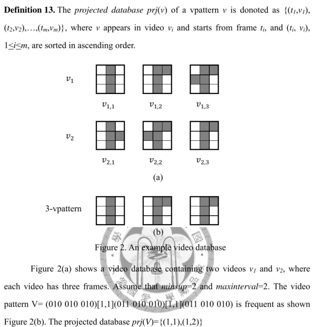
To generate all frequent spatterns, we first have to generate all possible candiadate 2-spatterns. Let us consider how to generate all possible candidate 2-spatterns for a video database with frame size of g×g.
Lemma 1. There are at most 2g2-2g possible candidate 2-spatterns in a video database with frame size of g×g.
Proof: For a frame size of g×g, if we fix the first pixel of the candidate 2-spattern at (1,1), we can generate (g2-1) candidate 2-spatterns since the pixel can be combine with the other pixel in the rest of cells to form a candidate 2-spattern. If we fix the first pixel of the candidate 2-spattern at (i,1), we can generate (g-1) candidate
13
2-spatterns since the pixel can be combine with the pixel in the first column except (1,1), 2<i<g. Therefore, we have (g2-1)+(g-1)*(g-1)=2g2-2g candidate 2-spatterns.
For example, we have 12 candidate 2-spatterns for a video database with frame size of 3×3, as shown in Figure 3.
Figure 3. Candidate 2-spatterns with frame size of 3×3
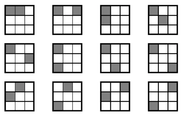
By scanning the video database once to count the support for each possible candidate 2-spattern, we can obtain all frequent 2-patterns and record the projected database of each frequent 2-spattern by using an rplist. Then, we put the rplists of those frequent 2-spatterns to the second level of the CV-tree, which is designed to store the patterns generated during the mining process.
Definition 15. Each node in the CV-tree is an rplist and has two kinds of children, that are used to record the video patterns grown in the spatial and temporal dimensions, respectively. The nodes grown in the spatial dimension are called s-nodes while the nodes grown in the temporal dimension are called t-nodes. The root of a CV-tree is a null pattern, {∅}. The pattern of the parent node of vpattern P is a sub-pattern of P.
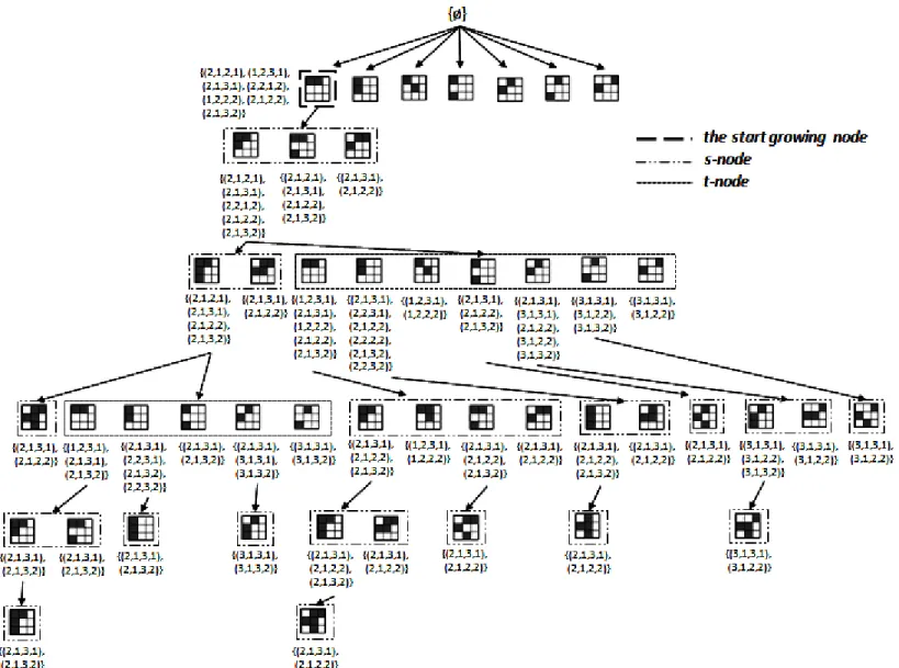
For example, the CV-tree shown in Figure 4 contains all frequent 2-spatterns in the example video database shown in Figure 2. The nodes of frequent 2-spatterns in the CV-tree are placed in the same order as they are generated, so do all k-patterns.
14
Figure 4. The CV-tree containing frequent 2-spatterns
3.2 Pattern generation
By joining two k-spatterns in the CV-tree, it generates a new (k+1)-spattern and the rplist of the new spattern is the intersection of rplists of two k-spattern. By using the rplist intersected, we can count the support of the newly generated spattern.
If the support is not less than minsup, we can add the rplist of the newly generated spattern to the CV-tree.
To join 2-spatterns P and Q in a video database with frame size of g×g, we have to shift the first pixel of P to match that of Q to avoid generating duplicate spatterns. If any pixel in the shifted P is greater than (g, g), we say that shifted P is not a valid pattern. Thus, the join operation is not allowed.
15
Definition 16. Any two frequent 2-spatterns S1 and S2 are joinable. The spattern of S1
joining to S2 is equal to S1∨S2, which is a 3-spattern, where ∨ is the logical OR operator for a bit-string. The rplist of the joined spattern is equal to the intersection of the rplists of S1 and S2.
For example, in Figure 4, the spattern of the first node (110 000 000) is joinable to (100 100 000) since the first pixels of both spatterns are at the same location. The intersection of the rplists of both spatterns are {(2,1,2,1), (2,1,3,1), (2,2,1,2), (2,1,2,2), (2,1,3,2)}. The joined spattern is equal to (110 000 000)∨(100 100 000)=(110 100 000), as shown in Figure 5(a), which is a 3-spattern with the support equal to 2. If minsup=2, the joined 3-spattern can be added to the CV-tree and becomes a child node of the node of (110 000 000).
Figure 5. Joining two spatterns
However, when the first pixels of both joining 2-spatterns are not at the same location, we fix the location of the latter 2-spattern and shift the former 2-spattern
(d) (c) (b) (a)
16
such that the location of first pixel of the former one is the same as that of the latter one. For example, to join both 2-spatterns (110 000 000) and (010 100 000) as shown in Figure 5(b), we shift the former spattern to (011 000 000) as shown in Figure 5(c) and then join both spatterns as shown in Figure 5(d). Finally, we can obtain a 3-spattern (011 100 000). Next we define a set of joinable nodes called joinable class.
Definition 17. Two frequent k-spatterns S1 and S2 are joinable if both share the first (k-1) pixels, k>3. The joined spattern is equal to S1∨ S2, which is a (k+1)-spattern. The rplist of the joined spattern is equal to the intersection of the rplists of S1 and S2. Definition 18. The joinable class of a frequent k-spattern S is JC(S)={S1,S2, …,Sn}, where S is joinable to Si and Si is a frequent k-spattern, k>2, 1<i<n. Note that the rplist of Si is a sibling node of the rplist of S. That is, the rplists of Si and S share the same parent in the CV-tree.
Definition 19. Two frequent k-vpatterns V1 and V2 are joinable if both share the first (k-1) spatterns, the last spatterns of both vpatterns are joinable, and all the time spans of both vpatterns are the same, k>2. The joined vpattern is obtained by replacing the the last spattern of V1 with the joined spattern of both last spatterns. The rplist of the joined spattern is equal to the intersection of the rplists of V1 and V2.
Definition 20. The joinable class of a frequent k-vpattern V is JC(V)={V1,V2, …,Vn}, where V is joinable to Vi and Vi is a frequent k-spattern, k>2, 1<i<n. Note that the node of Vi is a sibling of the node of V. That is, the nodes of Vi and V share the same parent in the CV-tree.
During the process of pattern generation, we first grow frequent video patterns in the spatial dimension and then grow them in the temporal dimension. To grow the frequent video patterns from a node of the CV-tree in the spatial dimension, we join the vpattern (P) of that node to each vpattern in P’s joinable class. If the joined pattern is frequent, it is added to the CV-tree and becomes the child node of node P. The procedure is repeated in a depth-first search manner until no more frequent vpatterns
17
can be found.
To grow the frequent video patterns from a node of the CV-tree in the temporal dimension, we first mine the frequent 2-spatterns in the projected database of the vpattern of that node so that the distance between the vpattern and each frequent 2-spattern mined is not greater than maxinterval. For each frequent 2-spattern mined, we append it to the vpattern to generate a new video pattern Q and compute the time span between the vpattern and 2-spattern. Next, we grow Q in the spatial dimension as the steps described above.
Let us consider how to mine vpatterns by a CV-tree as shown in Figure 6, where a part of the growing processes both in the spatial and temporal dimension is shown. In Figure 6, we use the example video database in Figure 2 to explain the process of growing patterns in the spatial and temporal dimensions. Assume that minsup=2 and maxinterval=2. After putting all frequent 2-spatterns to the second level of the CV-tree, we generate patterns from the first 2-spattern (110 000 000) The 2-spattern (110 000 000) can be joined to each pattern in its joinable class, namely, (100 100 000), (100 010 000), (100 000 100), (010 100 000), (010 000 100), (001 100 000). By joining (110 000 000) to each pattern in its joinable class, we obtain three frequent 3-spatterns, namely, (110 100 000), (110 000 100) and (011 100 000). We add these 3-spatterns to be the child nodes of node (110 000 000). Next, we grow the patterns from the 3-spattern node (110 100 000) in the same way and obtain two frequent 4-spatterns, (110 100 100) and (011 110 000). By joining both 4-spatterns, we obtain a 5-spattern node (011 110 010). At this point, we find that the joinable class of the 5-spattern is empty. Thus, no new spattern can be generated. Therefore, we finish growing the patterns in the spatial dimension.
Next, we start to grow the patterns in the temporal dimension. The projected database of the 5-spattern (011 110 010) is {(2,1,3,1), (2,1,2,2)}. We mine frequent 2-spatterns in the projected database so that the distance between every 2-spattern and
18
the 5-spattern is not greater than the maxinterval. Nevertheless, we cannot find any frequent 2-spattern in the projected database. Then, we backtrack to node (110 100 100) and grow the patterns from this node in the temporal dimension. The projected database of (110 100 100) is {(2,1,2,1), (2,1,3,1), (2,1,2,2), (2,1,3,2)}. We can mine five frequent 2-spatterns from the projected database, namely (110 000 000), (100 100 000), (100 000 100), (010 100 000), and (010 000 100). The projected database of the first frequent 2-spattern (110 000 000) is {(1,2,3,1), (2,1,3,1), (2,1,3,2)}. We compute the time span between the 4-spattern and the 2-spattern, which is [1,1]. Then we append the 2-spattern (110 000 000) to the 4-spattern to generate a new 2-vpattern, (110 100 100)[1,1](110 000 000). Similarly, we can find other four four 2-vpatterns as shown in Figure 6.
Then, we can grow the pattern from (110 100 100)[1,1](110 000 000) in the spatial dimension. We can obtain two 3-spatterns, (110 100 000) and (110 000 100), and one 4-spattern, (110 100 100). That is, we can obtain three v-patterns, (110 100 100)[1,1](110 100 000), (110 100 100)[1,1](110 000 100), and (110 100 100)[1,1](110 100 100). For each spattern obtained, we need to grow the patterns from it in temporal dimension. The steps described above will be recursively in a depth-first search manner until no more patterns can be found.
19
Figure 6. Growing patterns in the spatial and temporal dimensions
20
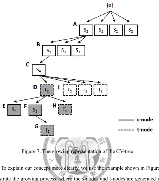
Figure 7. The growing representation of the CV-tree
To explain our concept more clearly, we use the example shown in Figure 7 to demonstrate the growing process, where the s-nodes and t-nodes are generated in the DFS manner recursively. In this example, we start from node A of a 2-spattern. Three s-nodes of 3-spatterns are generated from node A by joining the pattern of A to the patterns in its joinable class, where the joinable class of A contains the sibling nodes of A. Next, one s-node of a 4-spattern is generated from node B and no s-node can be grown from node C. Thus, we start to grow t-nodes by mining frequent 2-spatterns from the projected database of C so that the time span between the pattern of C and each frequent 2-spattern mined is not greater than maxinterval. Then, we append four frequent 2-spatterns mined to C and form four frequent 2-vpatterns, each of which consists of one 4-spattern and one 2-spattern.
For the vpattern of node D, we continue to generate two 3-spatterns E and F in the spatial dimension. No s-node and t-node can be generated from node E. Thus, E is
21
a leaf node. No s-node but one t-node G can be grown from node F to form a 3-vpattern. Then, we backtrack to node D and start to grow t-nodes from it. Since we can find a frequent 2-spattern H, a new 3-vpattern can be formed. Since H is a leaf node, we backtrack to node D then node C, and go to node I. The steps described above will be repeated in a depth-first search manner until no more patterns can be generated.
3.3 Closure checking and pruning strategies
We apply a similar concept used in CHARM [21] to perform pruning strategies and closure checking. There are two phases in our pruning strategies, namely, spattern pruning and vpattern pruning. We propose four rules in the first phase to prune unnecessary spatterns. In the second phase, we generate t-nodes only from the closed vpatterns or non-closed vpatterns with different projected database in the temporal dimension. After finishing the pruning strategies of both phases, we perform the closure checking for each possible vpatterns and output closed vpatterns.
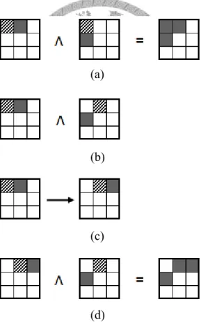
Let P and Q be two joinable k-spatterns in a joinable class C, and their projected databases be prj(P) and prj(Q), respectively. Let R be the pattern generated by joining P and Q, and prj(R) be the projected database of R. There are four kinds of relationships between prj(P) and prj(Q), namely, (1) prj(P) = prj(Q), (2) prj(P) ⊂ prj(Q), (3) prj(P) ⊃ prj(Q), and (4) prj(P) ≠ prj(Q). Based on these four relationships, we adopt four different ways to prune unnecessary spatterns.
1. If prj(P) = prj(Q), prj(R) = prj(P) ∩ prj(Q) = prj(P) = prj(Q). Thus, we can simply replace every occurrence of P with R, and remove Q’s rplist from the CV-tree since it is not closed.
2. If prj(P) ⊂ prj(Q), prj(R) = prj(P) ∩ prj(Q) = prj(P). We replace every occurrence of P with R.
3. If prj(P) ⊃ prj(Q), prj(R) = prj(P) ∩ prj(Q) = prj(Q). In this case, we add R’s
22
rplist to P’s joinable class, and remove Q’s rplist from C since R occurs in wherever Q occurs.
4. If prj(P) ≠ prj(Q), we cannot eliminate any pattern of both P and Q, just add R to P’s joinable class.
Figure 8 shows the four relationships and the corresponding pruning processes.
In Figure 8(a), if prj(P) = prj(Q), we replace P with the newly generated spattern R and delete Q from the CV-tree. Because Q’s projected database is as the same as P’s, R can be used to generate all possible spatterns which can be generated from Q. Then, the newly generated spattern will join to the spatterns in P’s joinable class. In Figure 8(b), if prj(P) ⊂ prj(Q), it means that P’s projected database is contained by Q’s. In this case, we replace P with the newly generated spattern R. In Figure 8(c), if prj(P) ⊃ prj(Q), it means that P’s projected database contains Q’s. We add R’s rplist to P’s joinable class and remove Q’s rplist from C, since R occurs in wherever Q occurs. In Figure 8(d), if prj(P) ≠ prj(Q), we cannot eliminate any pattern of both P and Q, just add R to P’s joinable class.
(a)
23
(b)
(c)
24
Figure 8. Four pruning strategies
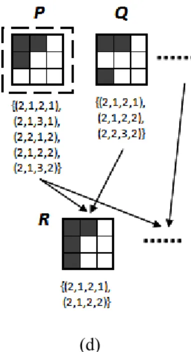
We only grow the vpatterns from a closed vpattern or a non-closed vpattern with different projected database in the temporal dimension. First, we check if the growing node is closed or it is non-closed but has different projected database with closed vpatterns. If this is the case, we grow t-nodes from it in the temporal dimension.
After an s-node is grown from a node, we put the newly generated vpattern to a closed pattern set and check if the new vpattern is closed. There are five cases as shown in Figure 9. First, if B contains A and the projected database of B also contains that of A, A is not closed, where A is a 1-vpattern in the CV-tree and B is a 1-vpattern in the closed pattern set. Thus, we mark node A in the CV-tree to indicate that it will not be grown in the temporal dimension, as shown in Figure 9(a). Second, if both A and B are the same and share the same projected database, A is not closed. Thus, we mark node A in the CV-tree to indicate that it will not be grown, as shown Figure 9(b).
Third, if A is contained by B and sup(A)=sup(B), but the projected database is not contained by that of B, A is not closed but it will still have to be grown t-nodes later, as shown in Figure 9(c). Fourth, if A contains B and the projected database of A contains that of B, A is added to the closed pattern set and B is removed from the closed pattern set at the same time, as shown in Figure 9(d). Finally, if A and B do not
(d)
25
contain each other, A is added to the closed pattern set, as shown in Figure 9(e).
Figure 9. Closure checking in vpattern pruning
3.4 The CVP algorithm
The CVP algorithm mines all frequent closed vpatterns in two dimensions, namely, spatial and temporal. It first grows frequent video patterns in the spatial dimension and then grows them in the temporal dimension. To grow the frequent video patterns from a node of the CV-tree in the spatial dimension, we join the vpattern (P) of that node to each vpattern in P’s joinable class. If the joined pattern is
Closed Pattern Set (a)
(b)
A
B A
(c)
(d)
{(1,2,1,1), (1,2,2,1), (2,1,2,2), (2,1,3,2)}
A
A
(e)
A
add
add
add {(1,2,2,1), (2,1,2,2), (2,1,3,2)}
{(1,2,2,1), (2,1,2,2), (2,1,3,2)}
{(1,2,2,1), (2,1,2,2), (2,1,3,2)}
{(1,2,2,1), (2,1,2,2), (2,1,3,2)}
{(1,2,2,1), (2,1,2,2), (2,1,3,2)}
26
frequent, it is added to the CV-tree and becomes the child node of node P. The procedure is repeated in a depth-first search manner until no more frequent vpatterns can be found.
To grow the frequent video patterns from a node of the CV-tree in the temporal dimension, we first mine the frequent 2-spatterns in the projected database of the vpattern of that node so that the distance between the vpattern and each frequent 2-spattern mined is not greater than maxinterval. For each frequent 2-spattern mined, we append it to the vpattern to generate a new video pattern Q and compute the time span between the vpattern and 2-spattern. Next, we grow Q in the spatial dimension as the steps described above.
The CVP algorithm is shown in Figure 10, which contains three functions:
CVPGrowth, GrowSNode and GrowSNode. They are shown in Figures 11, 12, and 13, respectively.
Algorithm: CVP
Input: a video database D, a minimum support threshold minsup, a maximum time span threshold maxinterval
Output: all closed vpatterns CV
(1) Scan the database D to find all frequent 2-spatterns, collect all frequent 2-spatterns found into C2, and add the rplist of each frequent 2-spattern found to the second level of the CV-tree;
(2) Let CV=∅;
(3) for each P in C2 do (4) CVPGrowth(P,CV);
(5) end for
(6) for each vpattern Q in CV do (7) Check if Q is closed;
(8) if Q is not closed then (9) Delete Q from CV;
(10) end if (11) end for (12) return CV;
Figure 10. The CVP algorithm
27
As shown in Figure 10, we first scan the video database to find all frequent 2-spatterns in step 1. For each frequent 2-spattern found, we call the CVPGrowth function to grow video patterns in both spatial and temporal dimensions. For each video pattern found, we check if it is closed. If this is the case, the video pattern will be added to CV.
Function: CVPGrowth
Input: a vpattern P, all closed vpatterns CV Output: all closed vpatterns CV
(1) Add P to CV;
(2) Cm+1=GrowSNode(P);
(3) if (Cm+1≠∅) then
(4) for each Q in Cm+1 do (5) CVPGrowth(Q,CV);
(6) end for (7) end if
(8) if P is a closed k-vpattern then (9) Cn+1=GrowTNode(P);
(10) if (Cn+1≠∅) then
(11) for each R in Cn+1 do (12) CVPGrowth(R,CV);
(13) end for (14) end if (15) end if
Figure 11. The CVPGrowth function
The CVPGrowth function consists of two parts. First, it calls the GrowSNode function to grow the video patterns in the spatial dimension. Then, it calls the GrowTNode function to grow the video patterns in the temporal dimension. For each newly generated video pattern, we recursively call the CVPGrowth function to grow video patterns in both spatial and temporal dimensions.
28
Function: GrowSNode Input: an m-vpattern P
Output: a set of (m+1)-spatterns Cm+1 (1) Let Cm+1=∅;
(2) for each S in JC(P) do (3) if S is joinable to P then
(4) Generate a (m+1)-vpattern T by joining P to S;
(5) If T is frequent, append the rplist of T to be a child node of P and add T to Cm+1;
(6) end if (7) end for (8) return Cm+1;
Figure 12. The GrowSNode function
In the GrowSNode function, we join P to every vpattern in P’s joinable class, where T is the vpattern generated by joining P to S. If T is frequent, we append T’s to be a child node of P in the CV-tree.
Function: GrowTNode Input: a vpattern P
Output: a set of 2-spatterns Cn+1 (1) Let Cn+1=∅;
(2) Mine the frequent 2-spatterns in P’s projected database so that the distance between P and each frequent 2-spattern mined is not greater than maxinterval.
Collect all frequent 2-spattern mined into C2. (3) for each S in C2 do
(4) Append S to P to generate a new vpattern Q;
(5) Compute the time span between the last two spatterns of Q and collect Q into Cn+1.
(6) end for (7) return Cn+1;
Figure 13. The GrowTNode function
In the GrowTNode function, we first mine all the frequent 2-spatterns in P’s projected database so that the distance between P and each frequent 2-spattern mined
29
is not greater than maxinterval. For each frequent 2-spattern mined S, we append it to P to generate a new vpattern Q and compute the time span between the last two spatterns of Q. That is, we compute the time span between P and S.
3.5 An example
In this section, we use the example database shown in Figure 2 and apply our proposed pruning strategies to illustrate how the CVP algorithm works to mine closed vpatterns. The process of growing s-nodes and t-nodes are already represented in Section 3.2 and Figure 6. We can get all frequent vpatterns if we continue growing as the manner explained in Figure 6. After applying our pruning strategies and the closure checking, we can get all closed vpatterns finally.
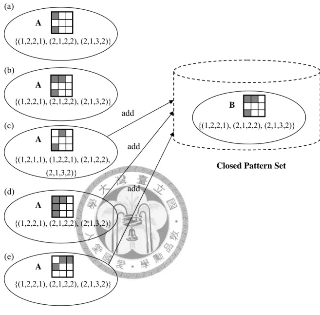
As demonstrated in Figure 14, from the first 2-spattern (110 000 000), three 3-spatterns can be grown and appended to it. Then, the spattern (110 000 000) can be viewed as a vpattern with length 1 and we add the 1-vpattern (110 000 000) to the closed pattern set and check if it is closed. Because the closed set is empty, we add it to the closed pattern set directly. In a DFS manner, we next grow the patterns from the 3-pattern node (110 100 000).
Since prj((110 100 000)) ⊃ prj((110 000 100)) and prj((110 100 000)) ⊃ prj((011 100 000)), we remove the nodes of (110 000 100) and (011 100 000) from the CV-tree but generate a new 4-spattern node (110 100 100) to be the child node of (110 100 000). After growing s-nodes for (110 100 000), we add it to the closed pattern set. Since the 1-vpattern (110 000 000) in the closed pattern set is contained by (110 100 000), we replace (110 000 000) with (110 100 000) in the closed pattern set and mark the node (110 000 000) in the tree to indicate that it is not closed and cannot be grown.
Figure 14. Growing closed vpatterns 30
31
Then, we grow the patterns from the 4-spattern node. Since prj((110 100 100))
⊃ prj((011 110 000)), we remove the 4-spattern node (011 110 000) and grow a new 5-spattern (011 110 010). Then we compare (110 100 100) with (110 100 000) which is in the closed pattern set, we find (110 100 000) is not closed and it is contained by (110 100 100) so we replace (110 100 000) with (110 100 100) in the closed pattern set. For the non-closed node (110 100 000) in the tree, prj((110 100 000)) is different from prj((110 100 100)) where (110 100 100) is a closed 1-vpattern in the closed pattern set so the node (110 100 000) still has to be grown in the temporal dimension later. Next, we continue growing the patterns from 5-spattern (011 110 010) and find that no s-nodes can be grown from this node. Since the newly generated 1-vpattern (011 110 010) is closed after the checking, we add it to the closed pattern set and replace the non-closed 1-vpattern (110 100 100). Then we try to grow t-nodes from the 5-spattern. However, no t-nodes can be grown. Thus, we backtrack to its parent node (110 100 100) and grows five t-nodes. From the first 2-spattern (110 000 000) in t-nodes, two 3-spatterns are generated. We delete nodes (100 000 100) and (010 000 100) from the CV-tree. Then, we add the 2-vpattern (110 100 100)[1,1](110 000 000) to the closed pattern set. We find this newly generated 2-vapttern is closed and it is added to the closed pattern set. At this time, there are closed 1-vapttern (011 110 010) and 2-vpattern (110 100 100)[1,1](110 000 000) in the closed pattern set. To grow the patterns from the generated 3-spattern (110 100 000), we find that prj((110 100 000))
= prj((110 000 100)). Thus, a new 4-spattern (110 100 100) is generated. Applying our pruning strategies, the 3-spattern (110 100 000) is replaced with the newly generated 4-spattern (110 100 100) as shown in Figure 14. Then we check if vpattern (110 100 100)[1,1](110 100 100) is closed. Since (110 100 100)[1,1](110 100 100) contains (110 100 100)[1,1](110 000 000), we replace the latter vpattern with the former one and mark the 2-spattern node (110 000 000) to indicate that it cannot be grown in the CV-tree. For the 4-spattern (110 100 100) in the CV-tree, no s-nodes can be grown and it is not closed. Thus, we mark it to indicate that it cannot be grown. Then we backtrack to node (110 000 000) which is marked. Thus, it cannot be grown in the
32
temporal dimension.
We have presented the growing process of the first 2-spatern (110 000 000) in the first level of the CV-tree. At this moment, we can get two closed 2-vpatterns in the closed pattern set, as shown in Figure 15.
Figure 15. Closed vpatterns in the closed pattern set
Similarly, we can repeat the above process in a depth-first search manner until no more vpatterns can be found. Finally, we can obtain four closed vpatterns, namely, (110 100 000)[1,1](011 110 010), (100 100 100)[1,1](011 110 010), (100 100 100)[2,2](110 100 100), and (100 100 100)[1,1](110 100 100)[1,1](110 100 100).
33
Chapter 4 Performance Evaluation
In this chapter, we conducted the experiments by using both synthetic and real datasets to our proposed method with the modified Apriori algorithm [1]. Both algorithms were implemented using Microsoft Visual C++ 2005. All the experiments were performed on an IBM compatible desktop with an Intel Core 2 6300 CPU @ 1.86GHz, 2.0 GB main memory, running on Microsoft Windows XP Professional.
Note that the support of a pattern is defined as the fraction of videos containing the pattern in the video database in the experimental section.
The modified Apriori algorithm contains three phases. First, we mine all frequent spatterns by using the Apriori property [1] level by level and collect all frequent 2-spattern into C2. Then, we check if each frequent spattern mined is closed and then delete non-closed ones.
Second, we generate all possible candidate 2-vpatterns by joining each closed spattern to each 2-spattern in C2, where the time spans between them include all the possible combinations of time spans so that each time span is not greater than maxinterval. Then, we scan the video database to count the support for each candidate 2-vpatterns generated. If its support is not less than minsup, it is frequent. For the frequent 2-vpatterns obtained, we expand their last spatterns by using the Apriori property level by level. Thus, we can obtain all frequent 2-vpatterns in the database.
Then, we check if each frequent 2-vpattern mined is closed and then delete non-closed ones.
Third, we generate all possible candidate k-vpatterns by by joining each closed (k-1)-vpattern to each 2-spattern in C2, k>2, where the time spans between them include all the possible combinations of time spans so that each time span is not greater than maxinterval. Then, we scan the video database to count the support for each candidate k-vpatterns generated. If its support is not less than minsup, it is
34
frequent. For the frequent k-vpatterns obtained, we expand their last spatterns by using the Apriori property level by level. Thus, we can obtain all frequent k-vpatterns in the database. Then, we check if each frequent k-vpattern mined is closed and then delete non-closed ones. The steps in the third phase are repeated until no more video patterns can be found.
4.1 Synthetic datasets
The synthetic generator used here is similar to the one used in Agrawal et al.
[1] with some modifications since the transaction here is a video. A video consists of a sequence of frames and we fix the frame size to be a square of 100×100. Table 1 lists the parameters and the default settings used in the synthetic data generator.
Table 1. Parameters used to generate synthetic data
Parameter Meaning Default setting
Number of videos in a video database 1,000
Average number of frames in a video 10
Average length of spatterns 8
Maximum time span threshold 2
Minimum support threshold 5%
Average number of potential patterns 50
Average length of spatterns in potential patterns 10
4.2 Performance evaluation on synthetic datasets
In this section, we compare our algorithm CVP with the modified Apriori algorithm by varying one parameter and keep other parameters at default values as shown in Table 1.
Figure 16 shows runtime versus minimum support threshold, where the minimum support threshold varies from 1% to 5%, the number of videos is 1000 and the average number of frames in a video is 10. The CVP algorithm runs 3-6 times
35
faster than the modified Apriori algorithm. The modified Apriori algorithm is more sensitive to minimum support threshold than the CVP algorithm. When the minimum support threshold decreases, the modified Apriori algorithm generates a large number of candidate patterns. However, the CVP algorithm localizes the support counting, pattern joining, and candidate pruning in the projected database. Therefore, the runtime of CVP algorithm increases slowly as the minimum support threshold decreases.
Figure 16. Runtime versus minimum support
Figure 17. Runtime versus number of videos
0 100 200 300 400 500 600 700 800 900
1 2 3 4 5
Runtime (sec.)
Minimum support (%)
Apriori CVP
0 500 1000 1500 2000 2500 3000 3500 4000 4500
2 4 6 8 10
Runtime (sec.)
Number of videos (K)
Apriori CVP
36
Figure 17 illustrates the runtime versus the number of videos, where the number of videos varies from 2000 to 10000, the average number of frames in a video is 10 and the minimum support threshold is 4%. When the number of videos increases, the runtimes of both algorithms increase nearly linearly and our CVP algorithm can run about 3 times faster than the modified Apriori algorithm.
Figure 18. Runtime versus maximum time span
Figure 19. Number of closed patterns versus maximum time span
0 100 200 300 400 500 600
1 2 3 4 5
Runtime (sec.)
Maximum time span
Apriori CVP
0 500 1000 1500 2000 2500 3000 3500
1 2 3 4 5
Number of closed patterns
Maximum time span
CVP, Apriori
37
Figure 18 illustrates the runtime versus maximum time span threshold. Figure 19 shows the number of closed patterns generated versus the maximum time span threshold, where the maximum time span threshold varies from 1 to 5, the number of videos is 1000, the average number of frames in a video is 10 and minimum support threshold is 5%. The CVP algorithm runs about 2.5 times faster than the modified Apriori algorithm. Both algorithms increase smoothly in runtime. As the maximum time span increases, the number of closed patterns also increases. However, the modified Apriori algorithm generates more unnecessary candidate patterns while maximum time span threshold increases so its efficiency is worse than the CVP algorithm.
Figure 20. Runtime versus number of frames
Figure 20 shows the runtime versus number of frames and Figure 21 illustrates the number of closed patterns versus number of frames, where the number of frames in a video varies from 10 to 30, the number of videos is 1000, the minimum support threshold is 5%. Also, both algorithms increase smoothly in runtime but the CVP algorithm runs faster. For the same reason, the modified Apriori algorithm generates more unnecessary candidate patterns while the number of frames increases hence it
0 200 400 600 800 1000 1200 1400
10 15 20 25 30
Runtime (sec.)
Number of frames
Apriori CVP
38
needs more time than the CVP algorithm. As shown in Figure 19, the number of closed patterns increases when the number of frames increases. That means there are more candidate closed patterns and we needs more time to check and prune.
Figure 21. Number of closed patterns versus number of frames
In summary, by using the pruning strategies and the pattern growth methods, the CVP algorithm can prune many non-closed patterns. The advantage of the CVP algorithm is that it can localize the support counting, pattern joining and candidate pruning in the projected databases. Therefore, the CVP algorithm is more scalable and efficient than the modified Apriori algorithm.
4.3 Performance evaluation on real datasets
The real dataset consists of 100 videos, where we extract a frame every second from a video. The videos are taken by ourselves. An example video containing three frames are shown in Figure 22, where each frame is transformed into a binary image with frame size of 20×20 as shown in Figure 23. The moving object marked in the video is a person throwing a ball.
0 500 1000 1500 2000 2500
10 15 20 25 30
Number of closed patterns
Number of frames
CVP, Apriori
39
Figure 22. A real video dataset Table 2. Parameters used in the real dataset
Parameter Meaning Default setting
Number of videos in a video database 100
Average number of frames in a video 3
Average length of spatterns 27
Maximum time span threshold 2
Minimum support threshold 5%
The default settings of the parameters used in the real dataset are shown in Table 2, where the average length of spatterns is 27, the maximum time span threshold is 2 and the minimum support threshold to 5%. Table 3 show the mining result of the real dataset by using our proposed algorithm. Figure 3 shows a pattern mined by our proposed algorithm. Because of the average length of spatterns of the dataset is 27, it is longer than synthetic datasets in Section 4.2. The modified Apriori algorithm will generate a large number of candidate patterns during the mining process. That leads to out of memory for the modified Apriori algorithm. Hence, we can compare our proposed algorithm with the modified Apriori algorithm by using this real dataset.
Frame 1 Frame 2 Frame 3
40
Table 3. Experiment results of a throwing-ball dataset
Total number of closed patterns 7,471
Average length of closed spatterns 15.47
Maximum length of closed spatterns 27
Average length of closed vpatterns 2.97
Maximum length of closed vpatterns 3
Total runtime 16214.1 sec.
Figure 23. A closed pattern mined
In Table 3, there are 7471 closed patterns mined. That means the CVP algorithm can mine the posture of throwing-balls in this experiment. Figure 23 shows one of the closed patterns mined. The mined closed pattern shows the movement of the object in the video and we can distinguish this kind of throwing-balls pattern from other movements.
The experimental results shows that the CVP algorithm is more scalable and efficient than the modified Apriori algorithm since it can localize the support counting, pattern joining and candidate pruning in the projected database.
41
Chapter 5 Conclusions and Future work
In this thesis, we proposed a novel algorithm, called CVP (Closed Video Pattern), to mine closed patterns in a video database. Our proposed algorithm consists of two phases. We first grow frequent video patterns in the spatial dimension and then grow them in the temporal dimension. By exploiting the CV-tree and rplists to store the information of frequent video patterns, the CVP algorithm can localize the candidate generation, pattern join, and support counting in a small amount of rplists.
During the process of pattern generation, we develop several pruning strategies to prune unnecessary or non-closed candidate patterns. Therefore, it can efficiently mine frequent closed patterns in a video database. The experimental results show the CVP algorithm is efficient and scalable, and outperforms the modified Apriori algorithm.
In the experiment conducted on the real dataset, the CVP algorithm is used to mine the patterns of throwing a ball. Besides that, the CVP algorithm can be used to find some interesting patterns in other applications, such as, action patterns, walking patterns, running patterns, swimming patterns, falling-down pattern, or getting-drowned patterns, etc.
However, the CVP algorithm is a memory-based algorithm. It would face the problem of out of the memory when the dataset is getting larger and larger. Therefore, how to develop a disk-based algorithm or an integrated algorithm of getting the balance of memory and disk is worth further study in the future. Moreover, the CVP algorithm generates a large number of candidate patterns during the mining process when the object is big or the number of frames is large. Thus, it is worth developing a modified CVP algorithm to promote the mining efficiency in the future.