Physicochemical speciation of bioactive trace metals (Cd, Cu, Fe, Ni)
in the oligotrophic South China Sea
Liang-Saw Wen
a,b,⁎
, Kuo-Tung Jiann
b, Peter H. Santschi
c aInstitute of Oceanography, National Taiwan University, P.O. Box 23-13, Taipei 106, Taiwan bNational Center for Ocean Research, National Taiwan University, P.O. Box 23-13, Taipei 106, Taiwan
cDepartment of Marine Sciences and Oceanography, Laboratory for Oceanographic and Environmental Research, LOER, Texas A&M University, 5007 Ave. U, Galveston, TX 77551, USA
Received 5 October 2004; received in revised form 14 January 2006; accepted 31 January 2006 Available online 20 March 2006
Abstract
Bioactive trace elements Cd, Cu, Fe, and Ni in the oligotrophic South China Sea (SCS) waters exhibit distinct chemical affinities and physical size distributions when using cross flow ultrafiltration and ion exchange techniques, even though they display similar nutrient-type distributions. Dissolved Cu (≤0.4μm) concentrations increased from 0.9nM in surface waters to 3nM at depths below 500 m, while those of dissolved Ni increased from 2 to 9 nM; those of dissolved Cd, from 0.01 to 0.9 nM; and those of dissolved Fe, from 0.1 to 0.7 nM. The majority of the dissolved Cd (∼100%) and Ni (>80%) concentrations were found in the ≤1kDa size fraction and as cationic labile forms. More than 50% of the total dissolved Cu in surface waters was in the ≤1kDa cationic labile form, while the non-exchangeable fraction that cannot be adsorbed by either cation or anion exchange resins increased from 28% at the surface to 50% below 500 m depth. Similarly, about 60% of total dissolved Fe in surface waters was in the≤1kDa fraction; the colloidal (1kDa–0.4μm) form of Fe was relatively constant throughout the water column, and amounted to 40% at the surface and 20% in deeper waters. Some fractions of the total dissolved Cu and Fe could be adsorbed by both cation and anion exchange resins, suggesting binding to“zwitterionic” molecules with both anionic and cationic binding sites. The cationic labile form of Fe tightly correlates with phosphate and nitrate, total dissolved Ni significantly correlates with silicate, and total dissolved Cd with phosphate, with different slopes in the upper 100 m than below. These correlations suggest a tight coupling of the cycling of these trace metals with those of individual nutrient elements. Biogeochemical and biophysical interactions between metals and organisms are not only through surface complexation to organic molecules of different molecular weights but they are also tightly coupled to colloidal aggregation due to their surfactant activity, properties that should be considered in future studies of oceanic elemental cycles.
© 2006 Elsevier B.V. All rights reserved.
Keywords: Trace metals; Speciation; South China Sea; Ultrafiltration; Chelex ion exchange; Cadmium; Iron; Copper; Nickel
1. Introduction
Nutrient-type trace elements such as Cd, Cu, Fe, Ni, are taken up by phytoplankton in surface waters and released back into the deep oceans through the oxidation
of organic matter (e.g., Bruland, 1980, 1994; Wong et
⁎ Corresponding author. Institute of Oceanography, National Taiwan University, P.O. Box 23-13, Taipei 106, Taiwan. Tel.: +886 2 3366 1381; fax: +886 2 3366 1685.
E-mail address:lswen@ntu.edu.tw(L.-S. Wen).
0304-4203/$ - see front matter © 2006 Elsevier B.V. All rights reserved. doi:10.1016/j.marchem.2006.01.005
al., 1983). Metal speciation, defined as the distribution of the element between different chemical species (Tessier and Turner, 1995), is the key to a better understanding of their availability to the biota and
mobility in the environments (Campbell, 1995; Simkiss
and Taylor, 1995). While only a small portion of the dissolved trace metals is present as truly free hydrated cationic species or complexes with inorganic ligands, a large fraction of many trace metals is complexed to
organic ligands (Wong et al., 1983; Buffle, 1988; Donat
and Bruland, 1995; Stumm and Morgan, 1996). In most cases, metal availability to phytoplankton is proportional to the free ion concentration of the metal (Sunda, 1994). Marine organisms regulate available metals in response to changing environmental condi-tions by excreting organic ligands that complex the metal and adjust the free metal ion concentration to
levels optimal for the growth of the organism (Morel
and Price, 2003and references therein). Phytoplankton can excrete both high-affinity, hydrophilic metal-specific complexing organic ligands, as well as biologically more resistant hetero-polycondensates
with numerous binding sites for trace metals (Leppard,
1995; Vasconcelos et al., 2002), some of them as
colloids with metal-complexing functionality (Leppard,
1995; Wen et al., 1996, 1999; Muller, 1996, 1999; Wells, 2002). Since the upper size for transport of molecules across bacterial cell walls is about 700 Da, colloidal ligands do not generally originate from cell
interiors (Payne, 1980), or pass across cell walls except
in cases of cell death or cell lysis caused by viral infections, especially in warm waters. According to
Agusti and Duarte (2000), cell lysis rates can be as high
as 1 day− 1 in warm surface waters. Under normal
circumstances, abundant mucus layers surrounding phytoplankton and bacterial cells are a constant source of trace metal complexing colloidal exopolymeric
substances, EPS (Leppard, 1995; Verdugo et al., 2004,
and references therein) and transparent exopolymeric
particles, TEP (e.g., Passow, 2002, and references
therein). These colloidal ligands also help to modulate free metal ion concentrations and thus influence the
availability of metals to organisms (Mackey and Zirino,
1994; Vasconcelos et al., 2002; Morel and Price, 2003). Earlier estimates of transport of available trace metal and reaction rates in the euphotic zone were based on
measurements of the operationally defined“dissolved”
fraction (≤0.4μm), which does not distinguish between
small soluble species and larger colloidal forms. The occurrence of trace elements in colloidal particles may decrease their bioavailability and increase their removal rates from the water column through colloidal pumping
(Honeyman and Santschi, 1989; Wen et al., 1997a,b). Thus, a key, but largely unanswered question, is how prevalent metal–colloid associations are in the water column of the oceans.
Investigations of biological availability of trace metals require means of determining the activities (or concentrations) of the free metal ions and other relevant
chemical species (Campbell, 1995). Electrochemical
voltammetric methods provide the most direct methods for the study of trace metal speciation at low concentration levels (nM to pM) because they do not normally require an initial step, such as preconcentration (Mota and Correia Dos Santos, 1995; Turner et al.,
1998). Many methods also exploit the complexation of
metal with competing ligands added to sample solution or the adsorption/desorption of metals on a surface of
chelating resins (Gledhill and van den Berg, 1994; Rue
and Bruland, 1995; Wu and Luther, 1995). The amount
of metal reacting with resin sites is often termed “the
labile fraction”. Accordingly, the classification of species as labile and non-labile depends on the nature of the added ligand and on the time taken for metals to partition or redistribute on a chelating resin. Voltam-metric methods are very useful in speciation studies to estimate complexing parameters such as stability constants and ligand concentrations. However, many difficulties still persist due to uncontrollable factors such as lability, irreversibilility, heterogeneity of the ligand, sorption of organics onto the electrode and the detection
window of the technique (Mota and Correia Dos Santos,
1995).
Chelating resins have seen considerable application in speciation studies, particularly the commercially available Chelex-100 resin, which is a styrenedi-vinylbenzene copolymer incorporating iminodiacetate
chelating groups (Apte and Batley, 1995). The
imino-diacetate groups coordinate metals by means of oxygen and nitrogen bonds similar to ethylenediaminetetraace-tic acid (EDTA), and the resins have a parethylenediaminetetraace-ticularly
strong affinity for trace metals.Riley and Taylor (1968)
first proposed to use Chelex-100 for the preconcentra-tion of total trace metals from seawater, then expanded rapidly in speciation studies following the findings of
Florence and Batley (1975, 1976, 1977) that the resin was selective and could be used to differentiate labile from non-labile fractions of trace metals. Chelex-100 retains free metal ions and loosely bound trace metals,
but not strong organic complexes (Fardy, 1992).
Although metal-ion retention by Chelex-100 is pH sensitive, and the labile trace metal fraction obtained is operationally defined at a pH of 5.5 in order to optimize
Fardy, 1992), it nevertheless provides an estimate of the
relative abundance of labile metal fractions (Donat et al.,
1994; Shafer et al., 2004). In addition, it provides for a simple and effective means of measuring labile metal
concentrations in aquatic systems (Figura and
McDuf-fie, 1979, 1980; Donat et al., 1994; Das et al., 2001; Guthrie, 2003; Öztürk and Bizsel, 2003).
Another important approach for speciation studies is the size-based separation methods such as dialysis, micro-filtration, ultrafiltration, and field-flow fraction-ation. These methods differentiate metals associated with colloids, e.g., nanoparticles and macromolecules, according to molecular sizes, molecular weight or
molecular diffusion rates (Muller, 1996; Wen et al.,
1999; Nishioka and Takeda, 2000; Nishioka et al.,2001;
Wu et al., 2001; Lyven et al., 2003). The link between molecular size and bioavailability is, however, more
tenuous and requires more investigations (Campbell,
1995; Muller, 1999; Wells, 2002).
In this study, we applied both operationally defined physical (cross-flow ultrafiltration) and chemical (ion exchange) separation techniques to determine the physicochemical speciation for bioactive elements Cd, Cu, Fe, and Ni in oligotrophic waters of the South China Sea (SCS), as well as its changes down the water column. Using this improved ultra-clean sampling and analytical methodology, we demonstrate, for the first time, that in the oligotrophic ocean, these four bioactive elements have distinctive characteristics of size distri-bution and chemical affinity, even though they all display similar nutrient-type vertical profiles.
2. Materials and methods 2.1. Study area
As central as the HOT and BATS programs are for
the Pacific and Atlantic time series studies (Karl and
Michaels, 1996), the SEATS (South East Asia Time-series Studies) program began in August 1998 by the National Center for Ocean Research of Taiwan at National Taiwan University, serves the same function for the South China Sea. SEATS provides for more comprehensive studies of the short and long-term
variability of biogeochemical processes (Wong et al.,
2002; Wu et al., 2003). The South China Sea is located in the tropical western North Pacific, extending from
the equator to 23°N and from 99°E to 121°E (Fig. 1).
It is the second largest marginal sea (with wide continental shelves and a deep basin reaching 4700 m) and receives runoffs from large rivers such as the Mekong River and Pearl River. On average, more than
10 typhoons pass through annually. Water circulation and ventilation are notably modulated by El Niño cycles, and affected by strong internal waves, internal
tides, inertia waves and alternating monsoons (Shaw,
1989; Shaw et al., 1996; Chao et al., 1996). The South China Sea connects to the open ocean through several passages, but only the Luzon Strait (sill depth of about 1900 m) effectively allows subsurface waters exchange with North Western Pacific waters. The Kuroshio, which flows northward to the east of Luzon Island, intrudes into the SCS through the Luzon Strait from
time to time, especially in winter (Shaw et al., 1996).
The residence time of South China Sea water is about
40–115 years (Broecker et al., 1986; Wang, 1986), and
the water column is permanently stratified. The oligotrophic shallow mixed layer is less than 50 m, diapycnal mixing is enhanced by the strong internal waves in the SCS basin. The mixing eliminates the oxygen minimum layer at depth and increases macronutrient concentrations in the upper 600 m, and produces a much shallower nutricline, distinctively
different from that of other oceans (Karl et al., 2001;
Wong et al., 2002; Wu et al., 2003). The annual deposition rate of atmospheric dust, which also delivers the limiting nutrient trace element Fe to the South China Sea, is the highest among oligotrophic waters, and occurs primarily from the fall through the
early spring during the northeast monsoon (Uematsu et
al., 1983; Merrill et al., 1989; Duce and Tinsdale, 1991; Husar et al., 1997). Thus, the availability of dust may also be the controlling factor for the biogeochem-ical cycles of associated trace elements in the South
China Sea (Fung et al., 2000; Wong et al., 2002; Wu et
al., 2003).
2.2. Sampling and analytical methods
Seawater samples were collected at the SEATS station, located at 18°N and 116°E during cruises of the R/V Ocean Researcher-I 639 (March 20–April 4, 2002),and R/V Ocean Researcher-I 711 (March 10–17,
2004) (Fig. 1). The bottom depth at station SEATS is
3980 m. Samples for trace metal speciation work were
collected either by a MITESS sampler (Bell et al., 2002)
attached to a ATE van suspended below a standard hydro-wire or by acid-cleaned Teflon-coated Go-Flo samplers (5 L, General Oceanics), attached on Kevlar wire with a modified epoxy coated CTD rosette and collected on the up-cast.
Water samples for nutrients and other measurements were collected on separate casts using a standard CTD rosette unit with 20 L Go-Flo samplers and collected on
the up-cast. Temperature and salinity were measured by a SeaBird, Model 911-plus CTD, with additional sensors used to measure chlorophyll fluorescence (Turner) and light transmittance (Wetlabs). The nutrients were mostly determined on board ship. Some samples
were also frozen in liquid N2until nutrient analysis in
the shore-based laboratory. Nitrite and nitrate were determined by the standard pink azo dye method
adapted for flow injection analyzer (Pai et al., 1990a).
Phosphate and silicate were determined with the standard molybdenum blue method with a flow
injection analyzer (Pai et al., 1990b). Additional
analysis of low concentration of phosphate in the upper euphotic zone (≤100m) were carried out with a modified MAGIC method only during March, 2002
expedition (Karl and Tien, 1992; Wu et al., 2003).
Dissolved oxygen was analyzed in discrete samples by a
colorimetric method (Pai et al., 1993), ammonium by an
improved indophenol blue method (Pai et al., 2001).
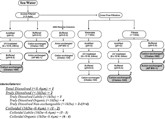
For physicochemical speciation analysis of metals, the processes of in-line filtration, cross flow ultrafiltra-tion and ion exchange chelating chromatography were Fig. 1. Sampling location in the South China Sea. The station of SEATS (18°N, 116°E) is indicated by the solid circle. The solid and the dotted lines, with arrows inside the South China Sea, show the current paths in summer and winter, respectively. Also shown is the main path of the Kuroshio, which intrudes into the South China Sea from time to time, especially in the winter.
all performed on board ship inside Class 100 laminar flow clean benches immediately after sample collection, to avoid any possible analytical and preservation
problems (i.e.,Wen et al., 1996, 1999, 2002;
Moliner-Martinez et al., 2003). Dissolved trace metal species determined in this study included two groups: physical species differentiated in size by ultrafiltration processes using a 1 kDa membrane, and chemical species differentiated by differential chemical affinity ion exchange chromatography.
Physical separation of total dissolved (≤0.4μm), truly dissolved (≤1kDa) and colloidal (1kDa–0.4μm) species were based on in situ in-line filtering through
acid-cleaned capsule filters (0.4μm, MSI) and
subse-quently ultra-clean cross flow ultrafiltration, CFUF (Wen
et al., 1996, 1999, 2002). A schematic of the analytical procedures employed and the definition of each metal
fraction in this study is shown inFig. 2. The cross flow
ultrafiltration system consists of regenerated cellulose 1-kDa cutoff membranes (Millipore), a peristaltic pump (Masterflex), a Teflon reservoir (Savillex), and Teflon tubings and connectors. The CFUF system was
rigor-ously calibrated and cleaned with successive rinses with different reagents (e.g., Q-HCl and Q-NaOH) and
distilled water as described previously (Wen et al.,
1996). Trans-membrane pressure was controlled at
20 psi and the concentration factor close to 10. Chemical separation of trace metals were carried out following a dual-column ion exchange technique, with details regarding method development described by
Jiann and Presley (2002). In general, this ion exchange separation/preconcentration technique utilized a cationic exchange column (Chelex-100, Bio-Rad) and an anionic exchange column (AG MP 1, Bio-Rad), connected in series to retain metal species with different chemical reactivity and affinity. A combination of Chelex-100 and AG MP-1 appeared to be able to separate labile (Chelex) and negatively charged organically bound (AG MP-1) fractions of metals. This extraction scheme is
well developed and documented (Liu and Ingle, 1989;
Fardy, 1992; Apte and Batley, 1995; Jiann and Presley, 2002; Jiann et al., 2005). The large concentration factor allowed by the ion exchange technique gives it an advantage over many other methods in determining
trace metal concentrations at low levels. Chelex-100 retains free metal ions and loosely bound trace metals, but not for metals that are strongly complexed with
organic compounds (Figura and McDuffie, 1979, 1980;
Morrison, 1987; Donat et al., 1994). AG MP1 resin, on the other hand, retains species that are negatively
charged, for example organic ligands (Liu and Ingle,
1989; Jiann and Presley, 2002). However, it also produces a non-exchangeable fraction that neither the cationic exchange (Chelex) nor the anionic exchange (AG MP1) column can retain. This non-exchangeable fraction includes complexes, such as metal–EDTA complexes or metal sulfides, that have very high
stability constants (Jiann and Presley, 2002; Jiann et
al., 2005). The labile trace metal fractions obtained by
Chelex-100 are operationally defined at a pH of 5.5 (Pai,
1988; Pai et al., 1990c; Fardy, 1992), which optimizes their kinetic stability. The application of a dual-column ion exchange using cationic (Chelex-100) and anionic (AG MP1) resins differentiates trace metal species by an easily handled, one-step preconcentration procedure that provides low blanks and high concentration factors. Inter-comparison studies had shown comparable results between voltammetry and the commonly used
Chelex-100 ion exchange technique in open ocean waters (van
Veen et al., 2002; Gardner and van Veen, 2004), even though ion exchange procedures have better detection
limits (Bruland et al., 1985; Fardy, 1992). Furthermore,
it provides a tool to investigate distribution of trace metal species and their reactivity in natural waters simultaneously. Trace metal species are thus operation-ally defined as cationic labile (Chelex-100 retained and deemed bioavailable) which has been defined earlier as
the bioavailable labile fraction (Donat et al., 1994; Apte
and Batley, 1995; Öztürk and Bizsel, 2003), organic–
anionic (AG MP 1 retained and deemed less bioavail-able), and non-exchangeable (not retained by either Chelex-100 or AG MP-1 column and deemed
unavail-able for plankton) (Fig. 2).
Firstly, both aliquots of filtered (≤0.4μm), and ultrafiltered (≤1kDa) were buffered (pH=5.5) by the addition of ammonia acetate (Seastar®, sub-boiled
acetic acid and ammonia solutions) immediately after collection and filtration. Secondly, the samples were passed through Chelex-100 columns first, and then through AG MP 1 column with flow rates controlled at 2.0 mL/min. After the samples passed through the column sets, the columns were disconnected, and the trace metals retained by the resins were eluted separately by washing each column individually with ammonia acetate buffer solution and Milli-Q distilled water to remove major cations and then with 2 N
HNO3 (Seastar®). Total metal concentrations in
aliquots of filtered (≤0.4μm), ultrafiltered (≤1kDa) and retentate samples (> 1 kDa) were first acidified immediately after collection (2 mL of sub-boiled
HNO3, Seastar®, per 1 L sample), then digested by
UV-irradiation (15W × 8, 12 h) and then buffered and pre-concentrated by Chelex-100 columns, a procedure
described previously inWen et al. (1996, 1999). Hence,
the dissolved“non-exchangeable” chemical fraction of
metal (with respect to the two ion exchange resins) was obtained as the difference between total metal concen-tration, and the sum of the fractions retained by cationic (Chelex-100) and anionic (AG MP 1) resins. Also, the ammonium acetate solution (10 mL), which passed through and was used as column wash agents was also collected and measured for trace metal concentration. In addition, fractions that were calculated by difference, and that show a fraction that is less than 1–10% of the total, depending on the metal and its concentration and
the statistical data given inTable 1, are not significant
(Fig. 2).
In addition to the normal ion exchange column setups, during the 2004 study, we had also reversed the sequence of ion exchange columns. Performed at the same time in parallel, separate water samples were passed through the anion exchange resins (AG MP 1) first, then the cation exchange resins (Chelex-100), as an additional analytical test procedure to identify the dissolved species that would
possibly behave both cationic and anionic,“zwitterionic”
or labile anionic complexes such as Cu citrate. Using this combination of physical (filtration and cross flow filtration) and chemical (ion exchange) separation Table 1
Analytical procedure blanks and extraction recoveries for trace metals studied (n = 5) Elements Analytical
procedure blank (ng)
NASS-5 reference material CASS-4 reference material
Certified (ng/L) Measured (ng/L) Recovery (%) Certified (ng/L) Measured (ng/L) Recovery (%)
Cd < 0.01 23 ± 3 22.8 ± 0.3 99 26 ± 3 25.5 ± 0.7 98
Cu 1.9 ± 0.4 297 ± 46 300 ± 4 101 592 ± 55 568 ± 8 96
Fe 4.3 ± 1.8 207 ± 35 211 ± 16 102 713 ± 58 706 ± 19 99
method, it is easy to operate on board ship to dif-ferentiate and characterize selected trace elements by chemical affinity and size in situ. Hence, the potential bioavailability through the water column can be determined, in terms of size distribution and chemical
reactivity in the ocean. Trace metal analyses were measured by graphite furnace atomic absorption spec-trometry (Varian, SpectrAA 880Z), equipped with an auto-sampler, pyrolized graphite furnace tubes, L'vov platforms, acid-cleaned Teflon sample cups, palladium matrix modifier, and Zeeman background correction. To assure consistency in data analyses, replicates were run and appropriate statistical analyses applied to the data, controls standards and certified reference materials (NASS-5, CASS-4) were used in every phase of experimentation. The analytical procedure blanks and recoveries of certified standard reference materials
NASS-5, and CASS-4 are listed in Table 1. The
recoveries ranged from 95% to 104% for the various elements in the different reference standards. Results for nutrients, chlorophyll a, and dissolved oxygen
concen-trations are reported in Table 2. Measured trace metal
concentrations in each fraction of collected seawater are
reported inTables 3 and 4for the different field studies.
For each field expedition, only eight different depths of sample water were collected for ultrafiltration for operation time consideration. For CFUF mass balance calibration, owing to the sample scarcity, only the retentates for sample water depth of 3500m (for March 2002) and 3000m (for March 2004) were used, and yielded mass balance of 99 ± 1% for Cd, 106 ± 2% for Cu, 85 ± 4% for Fe, and 104 ± 3% for Ni, while the rest of the colloidal retentate samples were desalted and freeze dried pending further isotopic and molecular analysis that will be reported elsewhere.
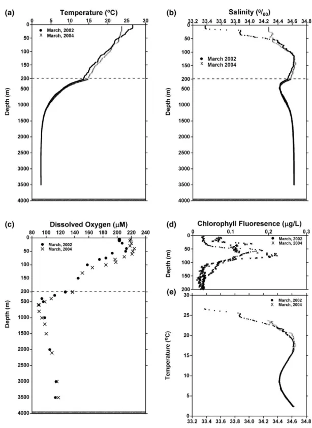
3. Results and discussions 3.1. Hydrographic conditions
Vertical profiles of temperature and salinity at the sampling location during March 2002 and 2004 are
shown in Fig. 3a and b. Even though these two field
expeditions were carried out during the same season in different years, distinctive differences in mixing depth and euphotic zone salinity distribution were observed. The deviations observed were possibly due to seasonal
circulation or an Ekman pumping effect (Wu et al.,
1999; Wong et al., 2002). General features include a shallow mixed layer depth (50 m in 2002 vs. 75 m in 2004), a steep thermocline in the surface layer of less
than 100 m, a salinity maximum (S > 34.6‰) at around
150 m, and a salinity minimum (S≈34.4‰) at around
500 m (Shaw, 1989; Shaw et al., 1996; Wong et al.,
2002). The concentrations of dissolved oxygen in the
upper layer (≤100m) were oversaturated or slightly undersaturated, with a subsurface maximum around 60– Table 2
Results of dissolved oxygen and nutrients analysis for collected seawater samples at station SEATS in the South China Sea during March 2002 and March 2004 sampling cruises
Depth (m) D.O. (μM) Nitrate (μM) Nitrite (μM) Ammonium (μM) Phosphate (μM) Silicate (μM) March 2002 5 203 N.D. N.D. 0.009 0.042 1.10 10 203 N.D. N.D. 0.001 0.022 1.70 20 207 N.D. N.D. N.D. 0.028 1.70 40 213 N.D. 0.01 0.005 0.042 1.79 50 212 0.04 0.07 0.051 0.05 2.10 60 193 1.40 0.18 0.081 0.15 4.20 75 184 3.64 0.10 0.047 0.22 8.60 80 175 3.98 0.07 0.023 0.25 9.54 100 158 10.6 0.04 0.009 0.72 12.0 150 145 13.3 N.D. N.D. 0.91 17.2 200 127 18.5 N.D. N.D. 1.26 28.1 300 112 24.3 N.D. N.D. 1.71 42.7 400 94 28.6 N.D. N.D. 2.02 56.7 500 96 30.5 – – 2.18 68.3 1000 98 36.2 – – 2.77 118 2000 105 37.5 – – 2.79 140 3000 114 37.1 – – 2.87 143 3500 113 37.3 – – 2.85 142 March 2004 5 219 N.D. 0.003 – 0.05 2.24 10 218 N.D. 0.005 – N.D. 2.24 20 220 N.D. 0.004 – N.D. 2.24 30 218 N.D. 0.007 – N.D. 2.24 40 224 N.D. 0.008 – N.D. 2.24 50 222 N.D. 0.007 – N.D. 2.24 60 221 0.14 0.007 – 0.05 2.24 70 210 2.00 0.113 – 0.15 5.23 80 197 1.98 0.101 – 0.20 7.46 90 198 2.70 0.026 – 0.26 4.48 100 184 3.40 0.022 – 0.41 7.46 110 165 8.09 0.001 – 0.67 8.96 130 151 10.6 0.001 – 0.77 12.7 200 137 16.9 N.D. – 1.28 26.1 400 107 27.6 N.D. – 1.90 44.8 500 98 30.5 N.D. – 2.20 66.4 600 89 33.1 – – 2.51 80.6 600 90 32.5 – – 2.35 79.9 800 90 – – – 2.66 100 1000 94 – – – 2.81 116 1200 98 38.3 – – 2.86 132 1500 100 38.6 – – 2.86 142 2100 108 38.6 – – 2.86 144 2500 – – – – – – 3000 115 38.5 – – 2.86 145 3500 117 38.5 – – 2.86 145
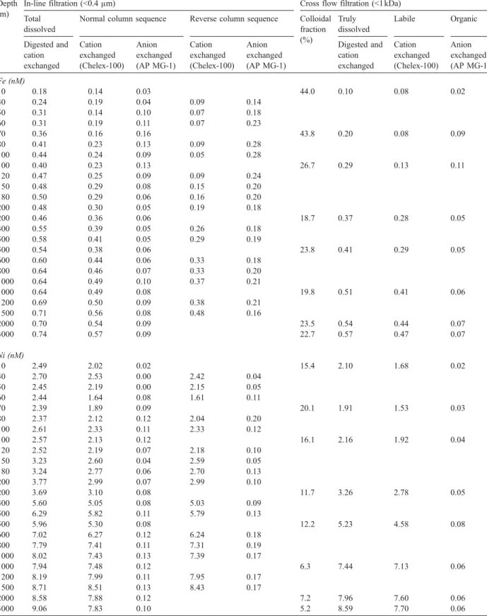
Table 3
Metal concentrations measured in different fractions of South China Sea waters collected at different depths during March 2002 expedition at SEATS station
Depth (m)
In-line filtration (<0.4μm) Cross flow filtration (<1 kDa)
Total dissolved Colloidal
fraction (%)
Truly dissolved Labile Organic
Digested and cation exchanged Cation exchanged (Chelex-100) Anion exchanged (AP MG-1) Digested and cation exchanged Cation exchanged (Chelex-100) Anion exchanged (AP MG-1) Cd (pM) 0 14 – – – – – 5 18 – – – – – 10 17 – – – – – 20 18 – – – – – 25 21 22 N.D. 0.0 21 21 N.D. 50 19 – – 60 21 20 N.D. 0.0 21 20 N.D. 75 85 – – 100 147 149 N.D. 1.4 145 147 N.D. 200 351 353 N.D. 2.0 344 346 N.D. 500 645 645 N.D. 1.1 638 639 N.D. 1000 792 794 N.D. 0.0 792 792 N.D. 2000 803 805 N.D. 1.0 795 797 N.D. 3000 816 – – – 3500 850 855 N.D. 1.2 840 841 N.D. Cu (nM) 0 0.78 – – – – – 5 1.02 – – – – – 10 1.07 – – – – – 20 1.22 – – – – – 25 1.19 0.75 0.11 12.6 1.04 0.63 0.08 50 0.96 – – – 60 0.91 0.39 0.17 12.1 0.80 0.31 0.14 75 0.92 – – – 100 0.93 0.31 0.18 10.8 0.83 0.25 0.14 200 1.04 0.38 0.19 0.98 0.33 0.17 500 1.35 0.48 0.34 8.1 1.24 0.42 0.23 1000 2.18 0.74 0.36 12.8 1.9 0.59 0.28 2000 2.70 0.91 0.45 13.7 2.33 0.79 0.34 3000 2.80 – – – – – 3500 2.91 1.00 0.47 14.8 2.48 0.88 0.35 Fe (nM) 0 0.19 – – – – – 5 0.18 – – – – – 10 0.18 – – – – – 20 0.22 – – – – – 25 0.24 0.2 0.03 37.5 0.15 0.11 0.03 50 0.27 – – – – – 60 0.34 0.17 0.1 26.5 0.25 0.12 0.07 75 0.39 – – – – – 100 0.41 0.22 0.07 24.4 0.31 0.14 0.05 200 0.45 0.29 0.06 0.38 0.23 0.05 500 0.56 0.39 0.03 16.1 0.47 0.32 0.02 1000 0.62 0.48 0.05 16.1 0.52 0.39 0.04 2000 0.66 0.56 0.08 18.2 0.54 0.45 0.07 3000 0.66 – –
70 m (Fig. 3c), which corresponded to the subsurface
chlorophyll a maximum (Fig. 3d). An oxygen minimum
was found at a depth of about 500 m during both study
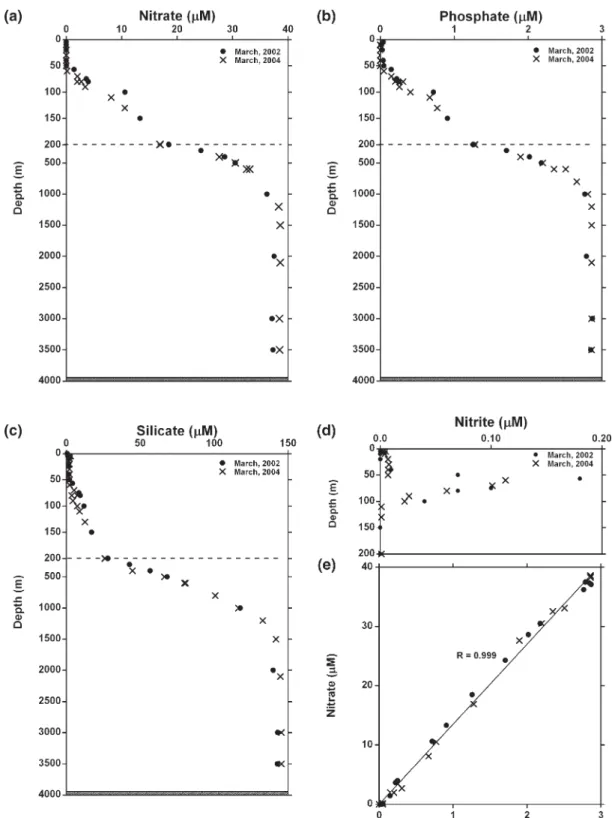
periods (Fig. 3d). The distributions of nitrate, phosphate,
silicate and nitrite are shown in Fig. 4. Nitrate was
depleted at the surface, with concentrations increasing sharply with depth from 50 m to 500 m, until they reached an almost constant level of 38μM below 2000m (Fig. 4a). Phosphate concentrations were about 22 nM at the surface. Below 1000 m, the concentrations of phosphate changed more gradually with depth until
they reached an almost constant level of 2.8μM below
2000 m (Fig. 4b). The primary nitrite maxima were both
located at the top of the upper nutricline, which corresponded exactly to the subsurface chlorophyll a maximum, an indication of nitrification, possibly strong
nitrogen fixation through biological activity (Fig. 4d).
Phosphate and nitrate show a systematic variation in response to surface water stratification with a N:P molar
ratio of 13.5 (Fig. 4e).
3.2. Physical speciation: vertical distributions of size
fractionated“dissolved” trace metals
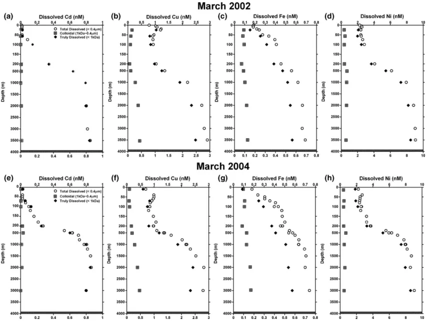
3.2.1. Cadmium
In this work,“dissolved” Cd concentration profiles,
studied during two separate field expeditions in the
South China Sea SEATS station, are shown inFig. 5a
and e. In 2002, Cd in the surface layer was almost depleted, with a minimum concentration of 0.014 nM at the surface; below that depth, concentrations increased
with depth to 0.79 nM at 1000 m, only slightly in-creasing from there to a maximum of 0.85 nM at 3500 m,
which is close to the bottom at 3980 m (Fig. 5a).
Comparable distributions were also found in 2004, however, total dissolved Cd concentrations found in the euphotic zone (shallower than 200 m) were generally about 15% lower, but with higher surface concentrations of 0.017 nM in the upper 10 m during year 2002 and
0.028 nM during year 2004 (Fig. 4b). Detailed physical
separation speciation analysis revealed that the great majority of the dissolved fraction of Cd was found in the truly dissolved (≤1kDa) fraction during both study
periods (Fig. 5a,e). These findings are similar to other
studies in oceanic environments (Wen et al., 1996, 1999;
Wells et al., 1998). 3.2.2. Copper
During March 2002, dissolved Cu concentrations were 0.78 nM at the surface, with a subsurface
maximum of 1.2 nM at a depth of 25 m (Fig. 5b).
Similar distributions were also found in March 2004, but with slightly lower surface concentrations, and a subsurface maximum of 1.0 nM at a depth of 50 m (Fig. 5f). Such Cu distributions in the euphotic zone have not been observed before, and the exact reasons will need further detailed investigations. Below 200 m, the concentrations of dissolved Cu changed more gradually with depth, until they reached an almost
constant level about 2.8 nM below 2000 m (Fig. 5b,f).
Concentrations of truly dissolved (≤1kDa) and colloi-dal (1 kDa–0.4μm) Cu show similar profiles at different Table 3 (continued)
Depth (m)
In-line filtration (<0.4μm) Cross flow filtration (<1 kDa)
Total dissolved Colloidal
fraction (%)
Truly dissolved Labile Organic
Digested and cation exchanged Cation exchanged (Chelex-100) Anion exchanged (AP MG-1) Digested and cation exchanged Cation exchanged (Chelex-100) Anion exchanged (AP MG-1) 3500 0.70 0.59 0.08 20.0 0.56 0.47 0.07 Ni (nM) 0 2.26 – – – – – 5 2.50 – – – – – 10 2.54 – – – – – 20 2.30 – – – – – 25 2.40 2.15 0.03 9.2 2.18 1.93 0.02 50 2.40 – – – – – 60 2.45 2.1 0.03 10.6 2.19 1.83 0.02 75 2.62 – – – – – 100 2.83 2.49 0.04 9.5 2.56 2.22 0.03 200 4.09 3.73 0.06 7.6 3.78 3.46 0.04 500 6.15 5.69 0.09 11.5 5.44 5.13 0.07 1000 7.94 7.23 0.10 8.3 7.28 6.65 0.05 2000 8.83 8.09 0.11 7.4 8.18 7.49 0.06
Table 4
Trace metal concentration measured in different fractions of South China Sea waters collected during March 2004 Ocean Research I-711 expedition at SEATS station
Depth (m)
In-line filtration (<0.4μm) Cross flow filtration (<1 kDa)
Total dissolved
Normal column sequence Reverse column sequence Colloidal fraction (%) Truly dissolved Labile Organic Digested and cation exchanged Cation exchanged (Chelex-100) Anion exchanged (AP MG-1) Cation exchanged (Chelex-100) Anion exchanged (AP MG-1) Digested and cation exchanged Cation exchanged (Chelex-100) Anion exchanged (AP MG-1) Cd (pM) 10 28 28 N.D. 6.9 23 26 N.D. 40 23 23 N.D. N.D. 20 50 22 22 N.D. N.D. 22 60 23 22 N.D. 23 N.D. 70 56 56 N.D. 3.6 53 54 N.D. 80 61 62 N.D. N.D. 58 100 101 100 N.D. N.D. 97 100 127 126 N.D. 4.0 123 121 N.D. 120 119 120 N.D. 3 119 150 163 162 N.D. 5 152 180 215 212 N.D. 2 210 200 274 295 N.D. 19 272 252 268 N.D. 200 271 278 N.D. 0.2 400 535 532 N.D. 18 510 500 632 627 N.D. 45 576 601 614 N.D. 500 628 624 N.D. 4.4 600 706 712 N.D. 44 660 800 718 706 N.D. 44 662 1000 807 784 N.D. 40 747 797 794 N.D. 1000 775 810 N.D. 4.4 1200 816 818 N.D. 50 761 1500 854 856 N.D. 48 802 2000 863 855 N.D. 5.5 849 838 N.D. 3000 800 811 N.D. 0.4 802 808 N.D. Cu (nM) 10 0.68 0.41 0.17 14.0 0.59 0.35 0.15 40 0.96 0.51 0.20 0.47 0.25 50 1.00 0.41 0.16 0.31 0.27 60 0.97 0.44 0.17 0.32 0.29 70 0.92 0.37 0.22 9.1 0.84 0.34 0.17 80 0.86 0.37 0.18 0.27 0.27 100 0.84 0.30 0.20 0.20 0.29 100 0.85 0.27 0.20 11.2 0.75 0.22 0.18 120 0.80 0.27 0.17 0.21 0.23 150 0.98 0.37 0.22 0.29 0.31 180 1.07 0.33 0.21 0.23 0.32 200 0.98 0.41 0.20 0.33 0.28 200 0.97 0.35 0.19 17.3 0.81 0.29 0.13 400 1.10 0.46 0.31 0.34 0.44 500 1.35 0.50 0.34 0.36 0.48 500 1.38 0.47 0.31 14.4 1.18 0.38 0.26 600 1.63 0.47 0.39 0.35 0.52 800 2.03 0.58 0.45 0.42 0.61 1000 2.20 0.68 0.45 0.47 0.66 1000 2.17 0.67 0.44 13.8 1.87 0.64 0.34 1200 2.33 0.79 0.51 0.58 0.72 1500 2.53 0.83 0.54 0.57 0.79 2000 2.82 0.95 0.56 14.2 2.42 0.89 0.41 3000 2.80 0.97 0.51 16.7 2.33 0.89 0.42
Table 4 (continued) Depth
(m)
In-line filtration (<0.4μm) Cross flow filtration (<1 kDa)
Total dissolved
Normal column sequence Reverse column sequence Colloidal fraction (%) Truly dissolved Labile Organic Digested and cation exchanged Cation exchanged (Chelex-100) Anion exchanged (AP MG-1) Cation exchanged (Chelex-100) Anion exchanged (AP MG-1) Digested and cation exchanged Cation exchanged (Chelex-100) Anion exchanged (AP MG-1) Fe (nM) 10 0.18 0.14 0.03 44.0 0.10 0.08 0.02 40 0.24 0.19 0.04 0.09 0.14 50 0.31 0.14 0.10 0.07 0.18 60 0.31 0.19 0.11 0.07 0.23 70 0.36 0.16 0.16 43.8 0.20 0.08 0.09 80 0.41 0.23 0.13 0.09 0.28 100 0.44 0.24 0.09 0.05 0.28 100 0.40 0.23 0.13 26.7 0.29 0.13 0.11 120 0.47 0.25 0.09 0.09 0.24 150 0.48 0.29 0.08 0.15 0.20 180 0.50 0.29 0.06 0.16 0.20 200 0.48 0.30 0.05 0.19 0.18 200 0.46 0.36 0.06 18.7 0.37 0.28 0.05 400 0.55 0.39 0.05 0.26 0.18 500 0.58 0.41 0.05 0.29 0.19 500 0.54 0.38 0.06 23.8 0.41 0.29 0.05 600 0.60 0.44 0.06 0.33 0.18 800 0.64 0.46 0.07 0.33 0.20 1000 0.64 0.49 0.10 0.37 0.21 1000 0.64 0.49 0.08 19.8 0.51 0.41 0.06 1200 0.69 0.50 0.09 0.38 0.21 1500 0.71 0.56 0.08 0.48 0.16 2000 0.70 0.54 0.09 23.5 0.54 0.44 0.07 3000 0.74 0.57 0.09 22.7 0.57 0.47 0.07 Ni (nM) 10 2.49 2.02 0.02 15.4 2.10 1.68 0.02 40 2.70 2.53 0.00 2.42 0.04 50 2.45 2.19 0.00 2.15 0.05 60 2.44 1.64 0.08 1.61 0.11 70 2.39 1.89 0.09 20.1 1.91 1.53 0.03 80 2.37 2.12 0.12 2.04 0.20 100 2.61 2.33 0.11 2.33 0.12 100 2.57 2.13 0.12 16.1 2.16 1.92 0.04 120 2.52 2.19 0.07 2.18 0.10 150 3.23 2.60 0.04 2.59 0.05 180 3.24 2.77 0.06 2.70 0.13 200 3.77 2.99 0.07 2.99 0.10 200 3.69 3.10 0.08 11.7 3.26 2.78 0.05 400 5.60 5.05 0.08 5.03 0.09 500 6.29 5.82 0.11 5.79 0.13 500 5.96 5.30 0.08 12.2 5.23 4.58 0.08 600 7.02 6.27 0.12 6.24 0.18 800 7.79 7.41 0.11 7.31 0.19 1000 8.02 7.43 0.13 7.39 0.17 1000 7.94 7.48 0.12 6.3 7.44 7.13 0.06 1200 8.19 7.99 0.11 7.95 0.17 1500 8.71 8.51 0.13 8.43 0.17 2000 8.58 7.88 0.12 7.2 7.96 7.60 0.06 3000 9.06 7.83 0.10 5.2 8.59 7.70 0.06
Fig. 3. Vertical profiles of (a) temperature, (b) salinity, (c) dissolved oxygen, (d) chlorophyll fluorescence and (e) T–S diagram in the water column for the March 2002 and March 2004 field expeditions to South China Sea waters at the SEATS station.
Fig. 4. Distribution of (a) nitrate, (b) phosphate, (c) silicate, (d) nitrite concentration, and (e) N/P molar ratio in the South China Sea at the SEATS station during March 2002 and March 2004.
Fig. 5. Vertical distribution of total dissolved (≤0.4μm), colloidal (1kDa–0.4μm) and truly dissolved (≤1kDa) trace metal concentrations in the water column for the 2002 field expedition to South China Sea waters at the SEATS station; (a) Cd, (b) Cu, (c) Fe, (d) Ni; for 2004, (e) Cd, (f) Cu, (g) Fe, (h) Ni. 11
7 W en et al. / Marine Chemistr y 101 (2006) 104 – 129
times. More than 80% of the Cu in surface waters was
present as truly dissolved species (≤1kDa). The
colloidal Cu concentration ranged from 0.2 to ∼0.5nM, which steadily increased with depth,
account-ing for an average 12–18% (Fig. 5b, f) in the dissolved
pool. It would seem that the colloidal forms of Cu are more refractory, as more low molecular forms of Cu also existed in the water column. These finding agree with some earlier studies that used either ion exchange or electrochemical techniques, which showed that dis-solved Cu in seawater appeared predominantly as low
molecular weight soluble organic complexes (Mills et
al., 1982; van den Berg, 1982; van den Berg et al., 1987; Moffett et al., 1990).
3.2.3. Iron
At the SEATS station, total dissolved Fe
concentra-tions were found to be ∼0.2nM in the surface layer,
which is very close to the solubility limit for Fe(OH)3
(Liu and Millero, 2002). Below the surface layer, the Fe
concentration sharply increased to ∼0.4nM at 100m
depth, and then changed more gradually with depth below 200 m until reaching an almost constant level of ∼0.7nM below 2000m during both sampling
expedi-tions (Fig. 5c and g). Concentrations of truly dissolved
Fe (≤1kDa) showed a similar profile, ranging from 0.1 to 0.6 nM. Colloidal Fe (1 kDa–0.4μm) concentrations were about 0.1 nM in the upper 100 m, with a minimum
of∼0.08nM found in both expeditions at 200m, below
which the concentrations increased very gradually. Concentrations of total dissolved and colloidal Fe were very consistent between the 2 years. The slightly higher (∼5%) value of deep waters in 2004 could be due to differences in sampling equipment (ATE vs. Go-Flo), or unknown analytical errors. About 50–60% of the
total dissolved Fe in surface waters was in the≤1kDa
fraction; the colloidal form was relatively constant throughout the water column, and amounted to 40% of the total dissolved concentration in the surface layer, and
∼20% in deeper waters (Fig. 5c and g). Recent studies
indicate that high molecular weight colloidal Fe often represents a large fraction of the dissolved Fe in marine
waters (Wen et al., 1999; Kuma et al., 2000; Barbeau et
al., 2001; Wu et al., 2001; Wells, 2002), a fraction that
cannot be directly utilized by phytoplankton (Rich and
Morel, 1990). Hence, Fe available for immediate algal uptake must originate from the low molecular weight,
truly dissolved fraction (Rich and Morel, 1990; Hudson,
1998). Siderophores, low molecular weight molecules
(0.3–1kDa), known to be released by some marine prokaryotes into the aqueous environment to bind Fe, tend to enhance Fe solubility, resulting in more available
Fe for biological uptake (Crumbliss, 1991; Reid et al.,
1993; Lewis, 1995; Rue and Bruland, 1995; Wilhelm et al., 1996; Hutchins et al., 1999a,b). Our findings agree
with earlier observations that≤1kDa species represent
a major fraction of total dissolved Fe in oceanic environments.
3.2.4. Nickel
Even though marine studies on dissolved Ni are limited, it appears that Ni is an essential micronutrient for some marine diatoms that use urea as a nitrogen
source (Wong et al., 1983; Jickells and Burton, 1988;
Price and Morel, 1991), and thus, Ni shows nutrient-like behavior. However, not much surface depletion of Ni
was ever observed (Bruland, 1980; Wong et al., 1983;
Mackey et al., 2002). During both years, total dissolved
Ni concentrations in SCS waters were 2–3nM in the
surface layer, increasing to∼8nM at a depth of 1000m,
below which they increased gradually towards the
bottom to about 9 nM at 3500 m depth (Fig. 5d and h).
The concentration of Ni in surface waters did not fall
below ∼2nM, even in the nitrate-depleted surface
waters. Low molecular weight (≤1kDa) forms of Ni concentrations were only slightly lower (ca. 10–20%) than those of total dissolved Ni, but with similarly shaped profiles in waters shallower than 500 m, with the remainder in the colloidal fraction. Below 1000 m, more
than 90% was in the≤1kDa fraction, and only a very
small fraction (∼10%) was in a colloidal form
decreasing with increased depth (Fig. 5d and h). In the
upper 100 m, profiles of Ni were similar to those of Cu, both in the 2002 and 2004 expedition, with a sub-surface maximum at depth of 25 and 50 m, respectively (Fig. 5d and h). Such distributions in the euphotic zone have not been reported before, and finding the exact reasons for such patterns would call for more detailed investigations.
3.3. Chemical speciation: affinity and potential
biolo-gical utilization for“dissolved” trace metals
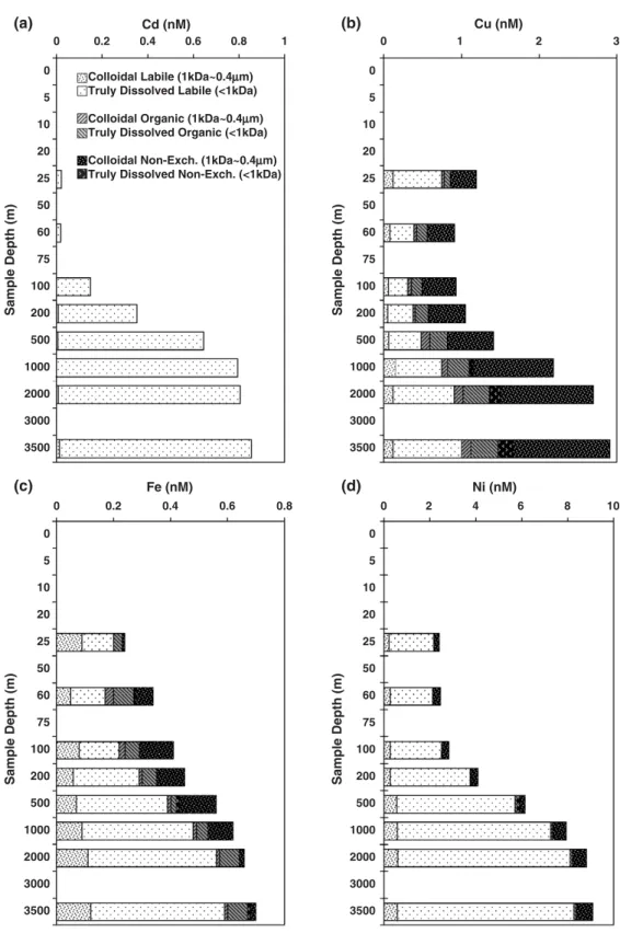
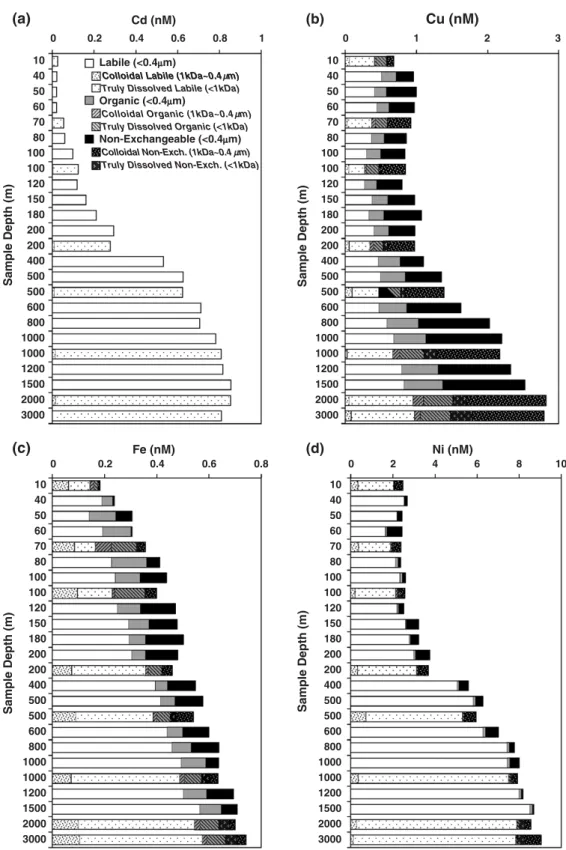
3.3.1. Cadmium
Cadmium can substitute for Zn in the enzyme carbonic anhydrase, allowing diatoms to maintain growth in Zn-deficient seawater, or even to be utilized
directly (Price and Morel, 1990; Lee et al., 1995; Sunda
and Huntsman, 2000; Cullen et al., 2003). The specific chemical forms of Cd in seawater are, however, not well
known (e.g., Das et al., 2001). In the SCS, vertical
distributions of the different forms of dissolved Cd with
different chemical affinities are shown in Figs. 6a and
0 0.2 0.4 0.6 0.8 1 0 5 10 20 25 50 60 75 100 200 500 1000 2000 3000 3500 Cd (nM) (a) Sample Depth (m)
Sample Depth (m) Sample Depth (m)
Sample Depth (m)
Colloidal Labile (1kDa~0.4µµm) Truly Dissolved Labile (<1kDa) Colloidal Organic (1kDa~0.4µm) Truly Dissolved Organic (<1kDa) Colloidal Non-Exch. (1kDa~0.4µm) Truly Dissolved Non-Exch. (<1kDa)
0 1 2 3 0 5 10 20 25 50 60 75 100 200 500 1000 2000 3000 3500 Cu (nM) (b) 0 0.2 0.4 0.6 0.8 0 5 10 20 25 50 60 75 100 200 500 1000 2000 3000 3500 Fe (nM) (c) 0 2 4 6 8 10 0 5 10 20 25 50 60 75 100 200 500 1000 2000 3000 3500 Ni (nM) (d)
Fig. 6. Dissolved trace metal concentration in different molecular weight (≤1kDa, and 1kDa–0.4μm) and chemical reactivity fractions (labile, organic, non-exchangeable), for the 2002 field expedition to South China Sea waters at the SEATS station; (a) Cd, (b) Cu, (c) Fe, (d) Ni.
0 0.2 0.4 0.6 0.8 1 10 40 50 60 70 80 100 100 120 150 180 200 200 400 500 500 600 800 1000 1000 1200 1500 2000 3000 Cd (nM) (a) Sample Depth (m)
Sample Depth (m) Sample Depth (m)
Sample Depth (m)
Labile (<0.4µµm)
Colloidal Labile (1kDa~0.4 m) Colloidal Labile (1kDa~0.4 m) Truly Dissolved Labile (<1kDa) Organic (<0.4µm)
Colloidal Organic (1kDa~0.4 m) Truly Dissolved Organic (<1kDa) Non-Exchangeable (<0.4µm)
Colloidal Non-Exch. (1kDa~0.4 m) Truly Dissolved Non-Exch. (<1kDa)
0 4 8 10 10 40 50 60 70 80 100 100 120 150 180 200 200 400 500 500 600 800 1000 1000 1200 1500 2000 3000 Ni (nM) (d) 0 0.2 0.4 0.6 0.8 10 40 50 60 70 80 100 100 120 150 180 200 200 400 500 500 600 800 1000 1000 1200 1500 2000 3000 Fe (nM) (c) 0 2 3 10 40 50 60 70 80 100 100 120 150 180 200 200 400 500 500 600 800 1000 1000 1200 1500 2000 3000 Cu (nM) (b) µ µ µ 1 2 6
Fig. 7. Dissolved trace metal concentrations in different molecular weight (≤1kDa, and 1kDa–0.4μm) and chemical reactivity fractions (labile, organic, non-exchangeable), for the 2004 field expedition to South China Sea waters at the SEATS station; (a) Cd, (b) Cu, (c) Fe, (d) Ni.
of Cd was in the≤1kDa cationic labile form. During the 2004 study, we also employed reverse sequence of ion
exchange columns. Results, tabulated in Table 4,
indicate that more than 90% of dissolved Cd showed zwitterionic behavior, i.e., it showed both cationic and anionic affinities, except at a depth of 60 m, corresponding to the chlorophyll maximum, where all of the dissolved Cd could be extracted by Chelex-100
but not by AP MG-1 (Table 4). In addition, these anionic
species of Cd extracted by the reversed column procedure were not found in the final acid eluant normally used, but in the ammonium acetate wash solution, which was used as a desalting agent. Even though voltammetric study in the Northeast Pacific revealed that in surface seawater, most Cd formed strong
complexes with natural organic ligands (Bruland, 1992),
this study suggests that dissolved Cd is mainly present as weak complexes or ionic pairs, confirming thermo-dynamic predictions that dissolved Cd is mostly present
as cadmium-chloride complexes (i.e., CdCl2, CdCl3−)
that are reactive and readily bioavailable (Stumm and
Morgan, 1996; Tessier and Turner, 1995). 3.3.2. Copper
Copper is well known to have a strong affinity for organic functional groups, which can be released as low molecular weight soluble organic complexes by
phytoplankton and bacteria (van den Berg, 1982; 1984;
van den Berg et al., 1987; Moffett et al., 1990; Gordon, 1992; Moffett and Brand, 1995; Leal et al., 1999; Gordon et al., 2000; Croot et al., 2000). In our 2004
study, dissolved cationic labile Cu (≤0.4μm) species
were found to be ∼0.6nM in surface waters, then
sharply decreased to ∼0.2nM at 100m depth, and
increased gradually with depth until they reached
∼0.9nM at 3000m (Fig. 7b). Concentrations of
dissolved anionic organic Cu (≤0.4μm) showed almost
a constant level of ∼0.2nM at depths shallower than
200 m, then gradually increased with depth, and very large fractions (25–50%) of dissolved Cu were found in the non-exchangeable forms, except in surface waters. In addition, during both 2002 and 2004 expeditions, more than 50% of dissolved Cu in surface
water was found in the≤1kDa cationic labile fraction.
A truly dissolved non-exchangeable fraction (≤1kDa, strongly complexed) was evident, which increased
from 15–20% at the surface to ∼40% below 500m
(Figs. 6b and 7b). Analysis also revealed that a large part of colloidal Cu (1 kDa–0.4μm) was actually cationic exchangeable, decreasing sharply over the
euphotic zone in the upper water column (from∼14%
to∼5%) while non-exchangeable colloidal Cu showed
an opposite trend, with more than 50% of colloidal Cu in the water deeper than 500 m being in non-exchangeable fractions, with only a minor part being
anionic exchangeable (Figs. 6b and 7b). Colloidal
organic copper remained at a low and almost constant level (∼4%) in the total dissolved pool of Cu throughout the water column. In addition, using reverse ion exchange column sets in 2004, we found that on average, 10% of the total dissolved Cu showed both cationic and anionic exchange ability, and a concen-tration distribution similar to that of colloidal Cu (Tables 3 and 4), indicating a polymeric and zwitter-ionic nature of the colloidal ligands. This study clearly demonstrated that the speciation of copper shows substantial variability down the water column due to complexation of copper to different types of organic ligands.
Midorikawa and Tanoue (1998) identified two Cu complexing carboxylic acid containing ligands, where-by the low molecular (≤1kDa) ligand was relatively weak and the stronger complex occurred in the higher
molecular mass fraction (1000–10,000 Da). Leal and
van den Berg (1998) demonstrated that Cu(I) is reversibly bound to organic species, and the concentra-tion of organic complexes can increase when either the ligand or the metal concentration is raised. Other studies
have also shown that a significant fraction of
“dis-solved” Cu in surface waters can not be released upon acidification to pH 2.0 but can be released months later, with UV oxidation eliminating this delay. This indicates that part of the organically complexed Cu is not in a dynamic equilibrium with the solution phase, but
remains kinetically inert (Sunda and Huntsman, 1991;
Wen et al., 1999).Wells et al. (2000)also reported that the distribution of such kinetically inert complexes is closely following the distribution of that of colloidal Cu, suggesting that the kinetically inert Cu is bound to colloidal complexes. Controlled laboratory experiments
with metal sulfides byJiann et al. (2005)suggested that
the kinetically inert Cu complex could be a Cu sulfide complex. Because of the very high stability of the
copper sulfide complexes (Stumm and Morgan, 1996),
and typical dissolved sulfide values ranging from 0.1 to
∼2nM in oxygenated seawater (Cutter and Krahforst,
1988; Luther and Tsamakis, 1989; Radford-Knoery and Cutter, 1994), similar to those of Cu, it is likely that Cu in SCS waters is bound to sulfide, with Cu and sulfide
controlling each other's speciation (Al-Farawati and
van den Berg, 1999). Our findings of that non-exchangeable-“inert” Cu mostly resided in ≤1kDa fraction agrees with the possible importance of sulfide complexes.
3.3.3. Iron
With the growing attention to iron dynamics in the marine ecosystem, there is also a greater interest in Fe
speciation (Martin, 1994; Wu et al., 2001; Sunda, 2001;
Gobler et al., 2002). During the 2004 expedition to the
SEATS station, Fe amounted to∼0.2nM in the surface
and∼0.75nM at 3000m depth (Fig. 7c), with more than
70% of total dissolved Fe below 200 m depth in a cationic labile form. Dissolved anionic organic Fe, as a smaller fraction, showed greater variability throughout the water column, with a distinct surface maximum (∼0.157nM) at a depth of ∼70m that corresponded to the chlorophyll and nitrite maximum. The non-exchangeable fraction of dissolved Fe showed higher concentrations below this depth. Using the reverse column technique, results showed that more than 40% of cationic Fe in waters shallower than 200 m can also occur as anions, with the largest fraction (∼78%) at 100 m near the nitrite maximum and coinciding with the
highest fraction of colloidal organic Fe (Fig. 7c).
Moreover, results of 2002 and 2004 studies further showed that about > 50% of the dissolved cationic labile Fe (≤0.4μm) in surface waters was found in the ≤1kDa fraction, which sharply increased below the surface; the
truly dissolved “non-exchangeable” fraction (≤1kDa
and not retained by either cationic or anionic exchan-gers) increased from 5% at the surface to a maximum of 30% at a depth right below that of the chlorophyll
maximum layer. Below 200 m, the ≤1kDa cationic
labile fraction gradually increased in deeper waters to
nearly 70%, and the “non-exchangeable” fraction
decreased to about 10%. The colloidal fraction was found mostly cationic labile, except at 70 m, where more than 50% of the colloidal Fe was found to behave
anionically (Figs. 6c and 7c). The concentrations of
these Fe fractions, especially the labile and organic ones, showed great variability down the water column.
The thermodynamically stable forms of dissolved Fe
(III) are species such as Fe(OH)2+and Fe(OH)4−, as well
as Fe(OH)30 that might be available for biological
uptake; colloidal FeOOH species, on the other hand, might not be bioavailable. Even though Fe(II) is more soluble than Fe(III), it will rapidly oxidize in oxygen-ated waters after microbially medioxygen-ated release into the
water (Rich and Morel, 1990; Kuma et al., 1996, 1998;
Millero, 1998; Liu and Millero, 2002). In addition, some organic compounds have been observed to either retard
or accelerate the process of Fe(II) oxidation (
Santana-Casiano et al., 2000).
While eukaryotic phytoplankton are found to
assim-ilate inorganic forms of dissolved Fe (Hudson and
Morel, 1990; Morel et al., 1991; Boye and van den Berg,
2000), low molecular weight organic ligands complex
more than 99% of dissolved Fe in seawater (Gledhill and
van den Berg, 1994; van den Berg, 1995; Rue and Bruland, 1995, 1997; Kuma et al., 1998), not only increasing Fe(III) solubility but likely also its bioavail-ability. Indeed, our results showed the existence of an organic anionic form of dissolved Fe in both the truly
dissolved and in the colloidal fraction (Fig. 6). The
processes responsible for availability of organic or inorganic Fe complexes for plankton are, however, still
being debated (Hutchins, 1995; Kuma and Matsunaga,
1995; Sunda and Huntsman, 1998; Kuma et al., 2000; Maldonado and Price, 2000). Zwitterionic siderophores, which are low molecular weight molecules (0.3–1kDa), can be released by some marine prokaryotes into the
water to bind Fe (Neilands and Nakamura, 1991; Reid et
al., 1993; Wilhelm and Trick, 1994; Wilhelm et al., 1996; Hudson, 1998; Hutchins et al., 1999a,b; Barbeau et al., 2001). Siderophores, which have conditional stability constants that match those of Fe-binding
ligands found in seawater (Lewis, 1995; Rue and
Bruland, 1995; Gledhill et al., 2004), tend to enhance
Fe solubility and bioavailability (Crumbliss, 1991; Trick
and Wilhelm, 1995). In addition, the weaker Fe binding ligand molecules found in seawater had conditional stability constants similar to zwitterionic Fe-porphyrin complexes (tetrapyroles), which are the most abundant
Fe chelators in cellular metabolism (Hutchins et al.,
1999a,b). Reports such as these could explain our findings of large fractions of dissolved Fe in zwitterionic
forms, as well as in a strongly complexed
“non-exchangeable” fraction that was highest in the upper
500 m of the water column, gradually decreasing below that depth, while the labile fraction increased with depth.
Nishioka and Takeda (2000) found that the growth of some plankton species in culture studies appeared to be stimulated by organic or inorganic colloidal Fe rather than soluble Fe species. Our study indicated that more than 80% of colloidal Fe (1 kDa–0.4μm) was indeed present as labile species, and the remainder as mostly in
organic (anionic exchangeable) forms (Fig. 6). This
suggests that even with high levels of Fe complexation, there might still be enough exchangeable free ionic Fe, with only a minor portion of dissolved Fe (10–30% as “non-exchangeable” species) that might not be available to phytoplankton.
3.3.4. Nickel
Nickel in seawater is thought to occur partly as stable organic complexes, with conditional stability constants
of about 1018(van den Berg and Nimmo, 1987; Nimmo
Berg, 1997). It was also found that strong Ni-organic complexes made up a significant fraction of the total dissolved Ni in estuarine and coastal environments (Nimmo et al., 1989; Turner et al., 1998; Wen et al.,
1999). However, interactions of Ni(II) with dissolved
organic matter have not been well studied (Das et al.,
2001; Wells, 2002; Mandal, 2002). It is not clear whether Ni occurs as weak organic or as inorganic complexes. In this work, more than 85% of the total dissolved Ni was found in the truly dissolved labile fraction (≤1kDa cationic exchangeable), with a very
small fraction (∼5%) bound to colloids (Figs. 6d and
7d). Surprisingly, contrary to the other elements we
investigated, less than 3% of these cationic forms of Ni can also behave as anions. The very small anionic organic Ni fraction in this study, compared with other
studies (Nimmo et al., 1989; Turner et al., 1998; Wells et
al., 2000) could be due to the oligotrophic character of the South China Sea, or due to differences in analytical methods employed. However, the organic Ni maximum that was observed at the corresponding depth of the nitrite (and chl. a) maximum would argue that the method could detect this anionic organic species in more productive regions as well. The percentage of the labile Ni fraction was similar in the surface layer as in the deeper waters, and the minimum appeared at the corresponding depth of the chlorophyll a maximum. These results suggest biological uptake of Ni, and active interaction with living phytoplankton. In a recent study
of the western equatorial Pacific,Mackey et al. (2002)
found that the concentration of Ni also did not fall below 2 nM in the surface water, where primary production is strongly dependent on recycled nitrogen (mainly ammonia and urea). These authors proposed that this residual Ni is not bioavailable and that Ni could be biolimiting, since the metabolism of urea requires the nickel-containing enzyme urease. Our findings of 10% to 20% of the total dissolved Ni in the South China Sea
appeared to be in the“non-exchangeable” fraction (both
in truly dissolved and colloidal sizes), in agreement with
the conclusions drawn byMackey et al. (2002).
3.4. Correlations of nutrients and trace metals: proxies for nutrient cycles
A clear linearity in the plot of Cd–PO4 has been
generally reported, with slopes around 0.3–0.36 (nM
Cd/μM PO4) in the Pacific Ocean (Boyle et al., 1976;
Bruland et al., 1978; Bruland, 1980; Kudo et al., 1996; Abe, 2002). This correlation is widely used as a paleo-nutrient proxy that exploits Cd that is preserved in fossil foraminifera for the determination of historical
phos-phate concentration in ocean surface waters (Boyle et
al., 1976; Bruland et al., 1978; Hester and Boyle, 1982; de Baar et al., 1994). In this work, the concentration of
PO4was less than 0.5μM in the shallow mixed layer of
less than 50 m in depth above the chlorophyll a
maximum, and the Cd/PO4ratio was found to be only
0.028 nM/μM (Fig. 8). This value is much smaller than
the regeneration ratio of Cd to PO4 found by other
studies of Pacific Ocean's surface waters (Kudo et al.,
1996; Abe, 2002). Below 100 m in our study area, the
Cd/PO4ratio averaged 0.297 nM/μM, and Cd correlated
with NO3, with a Cd/NO3 ratio of 0.021 nM/μM,
comparable to other published results.
Total dissolved Fe concentrations displayed a sig-nificant covariance with nutrient elements, with the cationic labile fraction of iron showing the strongest
Fig. 8. Correlation of total dissolved cadmium concentration to that of dissolved phosphate and nitrate found in South China Sea waters at the SEATS station.
correlation with phosphate and nitrate (Fig. 9). Because Fe is involved in numerous biochemical uptake and regeneration processes as an essential micronutrient for phytoplankton growth, such relationships could be expected. The preferential uptake of Cd and Fe by phytoplankton in the surface euphotic zone and the re-mineralization processes in the deeper waters are the main factors for the difference in observed correlations. As a consequence, these processes cause the Fe/Cd correlation in the euphotic zone ([Fe] = 0.193 + 2.216 × [Cd], R = 0.520), which is different from that in deeper waters ([Fe] = 0.342 + 0.407 × [Cd], R = 0.948). Howev-er, a similar Fe/Cd ratio was found for both total
dissolved and cationic labile fractions in this work (Fig.
10), suggesting similar production and regeneration
processes for Fe and Cd. Hence, the removal processes are not only regulated by marine organisms but also by
the coupling of chemical (e.g., thermodynamics and kinetics) and physical (e.g., diffusion and aggregation) processes. As the affinity for trace metals as micro-nutrients to various planktons uptake are likely species dependent, our results thus argue against the use of empirical models, which assume fixed phytoplankton uptake ratios that can be taken from any water column for any dissolved metal/nutrient ratio, without
consid-ering the effect of metal speciation (Saager and de
Baar, 1993; Elderfield and Rickaby, 2000; Cullen et al., 2003).
A plot of total dissolved Ni versus Si resulted in a strong linear correlation of Ni with Si in the South China
Sea (Fig. 11). Linear correlations between Ni and Si
Fig. 9. Correlation of total dissolved and dissolved cationic labile Fe concentration to that of dissolved phosphate and nitrate found in South China Sea waters at the SEATS station.
Fig. 10. Correlations of Fe and Cd concentrations in different fractions found in South China Sea waters at the SEATS station.
Fig. 11. Correlation of total dissolved Ni concentration to that of dissolved silicate found in South China Sea waters at the SEATS station.
have also been demonstrated in the waters of the North
Pacific (Sclater et al., 1976; Bruland, 1980; Jones and
Murray, 1984), the Indian Ocean (Danielsson, 1980; Saager et al., 1992) and the western equatorial Pacific (Mackey et al., 2002). However, Ni only correlated with
PO4and NO3in the euphotic zone (≤100m depth), and
no strong correlation was found below 200 m. These findings strongly suggest active uptake by biotic processes for dissolved Ni in surface waters and only partial release at greater depth occurring through different pathways.
4. Conclusions
Using cross flow ultrafiltration and ion exchange chelating techniques, we investigated chemical and physical speciation of Cd, Cu, Fe and Ni in the oligotrophic South China Sea. Dissolved Cd concentra-tions in surface waters ranged from 0.01 to 0.9 nM, with
the majority residing in the ≤1kDa labile form,
increasing to ∼3nM at depths below 500m. More
than 50% of Cu in surface water resided in smaller than 1 kDa labile forms. The strongly complexed non-exchangeable form increased from 28% at the surface to 50% below 500 m; the colloidal form (1 kDa–0.4μm)
of Cu was relatively constant, and averaged ∼16% of
the total dissolved Cu pool. The concentrations of dissolved Fe increased with depth from surface water concentrations of 0.1 to 0.2 nM, which is near-saturation
with Fe oxyhydroxides in seawater (Liu and Millero,
2002), to∼0.7nM in the bottom waters. About 50% of
total dissolved Fe (≤0.4μm) in surface water was found
in the≤1kDa cationic-labile fraction. Below 200m, the
≤1kDa cationic-labile fraction gradually increased to nearly 70% in deeper waters. This fraction linearly correlated with phosphate and nitrate throughout the water column, likely indicating a recycled fraction of Fe.
The truly dissolved “non-exchangeable” fraction
(≤1kDa and not retained by either cationic and anionic exchangers) increased from 5% at the surface to a
maximum of 30% at a depth of ∼60m, which
corresponded to the depth of chlorophyll a and nitrite maximum. The colloidal fraction of Fe was relatively constant throughout the water column, amounting to 40% at the surface and 20% in deeper waters. Dissolved Ni varied from 2 to 9 nM, with more than 80% residing
in≤1kDa labile forms, and a very small fraction (∼5%)
in colloidal forms.
Significant fractions of the total dissolved Cu and Fe were adsorbed by both cationic and anionic exchange resins, which also showed similar concentration dis-tributions to those of colloidal fractions, thus suggesting
that some fraction of these metals was possibly complexed by zwitterionic ligands. Strong correlations were also documented between phosphate, nitrate and Cd (albeit with different slopes for the upper 100 m and for depths below), as well as to labile cationic Fe. In addition, Ni correlated well with silicate. These correlations suggest that these bioactive elements are all affected by enzymatically controlled biotic uptake processes in the euphotic zone and subsequent re-mineralization processes down the water column. Dissolved trace elements in seawater are much more dynamic than previously thought and biochemical and biophysical interactions through organic complexation that are coupled to colloidal aggregation should be considered in future studies of ocean elemental cycles. Acknowledgements
We would like to thank Miss Wen-Hui Li, Lee-Ying Wu, Jia-Ying Chuang, I-Ting Jiang and research assistants of the Chemistry Laboratory of National Center for Ocean Research for help with the sampling and ancillary analysis, and Dr. C.-M. Tseng provided the nutrient data of March 2004 expedition. The assistance of crew and technician on board research vessel Ocean Research-I during the sampling expeditions is greatly appreciated. We thank Dr. James Moffett and two anonymous reviewers for their insightful comments and suggestions that helped improve the manuscript. This research was, in part, supported by the National Science Council grant NSC-89-2611-M-002-054, NSC-90-2611-M-002-024, NSC-91-2611-M-002-07 and Nation-al Center for Ocean Research.
References
Abe, K., 2002. Preformed Cd and PO4and the relationship between the two elements in the northwestern Pacific and the Okhotsk Sea. Marine Chemistry 79, 27–36.
Achterberg, E., van den Berg, C., 1997. Chemical speciation of chromium and nickel in the western Mediterranean. Deep-Sea Research II 44 (3–4), 693–720.
Agusti, S., Duarte, C.M., 2000. Strong seasonality in phytoplankton cell lysis in the NW Mediterranean littoral. Limnology and Oceanography 45, 940–947.
Al-Farawati, R., van den Berg, C.M.G., 1999. Metal-sulfide complex-ation in seawater. Marine Chemistry 63, 331–352.
Apte, S., Batley, G.E., 1995. Trace speciation of labile chemical species in natural waters and sediments: non-electrochemical approaches. In: Tessier, A., Turner, D. (Eds.), Metal Speciation and Bioavailability in Aquatic Systems. John Wiley and Sons, pp. 259–306.
Barbeau, K., Rue, E., Bruland, K., Butler, A., 2001. Photochemical cycling of iron in the surface ocean mediated by microbial iron (III)-binding ligands. Nature 413, 409–413.