隱式最近點方法求解在變動曲面上的對流擴散方程

國

立

交

通

大

學

應用數學系

碩

士

論

文

隱式最近點方法求解在變動曲面上的對流擴散方程

An implicit closest point method for solving

convection-diffusion equations on a moving surface

研 究 生：成澤仕軒

指導教授：賴明治 教授

隱式最近點方法求解在變動曲面上的對流擴散方程

An implicit closest point method for solving

convection-diffusion equations on a moving surface

研 究 生：成澤仕軒

Student：Narisawa Shinoki

指導教授：賴明治 Advisor：Ming-Chih Lai

國 立 交 通 大 學

資 訊 科 學 系

碩 士 論 文

Submitted to Department of Applied Mathematics College of Science

National Chiao Tung University in partial Fulfillment of the Requirements

for the Degree of Master

in

Applied Mathematics

June 2013

Hsinchu, Taiwan, Republic of China

隱式最近點方法求解在變動曲面上的對流擴散方程

學生：成澤仕軒

指導教授

賴明治

國立交通大學應用數學系﹙研究所﹚碩士班

摘

要

本文提出一個數值計算方法去求解變動曲面上的對流擴散方程。利

用水平集函數捕捉變動曲面。根據最近點方法，利用最近點將對流擴

散方程延拓到曲面附近的小區域，並且在這小區域上用 Crank-Nichoson

方法求解嵌入方程。

i

An implicit closest point method for solving

convection-diffusion equations on a moving surface

student：

Advisors：Ming-Chih Lai

Department﹙Institute﹚of

National Chiao Tung University

ABSTRACT

We propose a numerical method to solving convection-diffusion equation on a

moving surface. We use the level set function to capture the deforming surface.

Based on the closest point method, we extend the convection-diffusion equation

into a small neighborhood of the surface by closest point, and use Crank-Nicolson

scheme to solving the embedding PDE on the neighborhood of the surface.

誌

謝

本論文的完成，首先感謝我的指導教授賴明治老師。在教授的指導下，讓

我逐漸熟悉數值偏微分方程及科學計算方法。使我在數值方法及科學計算領域

中，找到我的興趣以及研究做出的成就感。老師不只引導我學習應有的態度，並

且教導我們做人的道理，相信往後的人生道路上將會受用無窮。並感謝胡偉帆學

長與陳冠羽學長，教導我許多知識，在學業上對我有極大的幫忙。

感謝曾經教導過我的教授，你們不僅傳授我數學上的知識，還有學習應有

的態度。在論文口試期間，承蒙吳金典教授與黃聰明教授費心審閱並提供許多寶

貴的意見，使得本篇論文更加完備，學生銘記在心。

感謝我周遭所有同學兩年來的相處，一起學習，一起玩樂，一起成長。在

我低潮的時候，需要幫忙的時候，總是有你們陪伴。我不會的東西很多，許多事

情都是你們教我的，感謝有你們的陪伴與包容。你們讓我研究生涯過的多采多

姿，充滿樂趣。謝謝你們。

最後，我要感謝我的父母，有你們的支持，我才能順利地完成學業，你們

是我最堅強的後盾，讓我無憂無慮的學習。願與所有關心我的人，一同分享此篇

論文完成之喜悅與榮耀。

iii

中文提要

目 錄

………

i

英文提要

………

ii

誌謝

………

iii

目錄

………

iv

一、

Intorduction………

1

二、

Surfactant concentration equation………

2

三、

The closest point method………

3

四、

Level set representation………

6

五、

Numerical method………

7

六、

Numerical results………

14

七、

Conclusion………

24

Appendix

………

24

1

Introduction

Solving PDEs on a moving and deforming surface is important. There are many applica-tions in fluid dynamics, material science, and the mathematics of images. For example, the convection-diffusion equation on a moving surface can be used to describe the surfactant which is convected by flow and diffused along the surface. It is important for the immiscible fluids problem which has surfactant on the interface between different fluids. The surface tension depends on the surfactant concentration, and it will effect the flow around the in-terface and deform the inin-terface. To solve this problem, we need to capture the deforming surface. In the literature, there are some methods to capture a deforming surface, includ-ing front-trackinclud-ing method[12], volume-of-fluid method[13], level set method[7], Arbitrary Lagrange-Euler method[14],etc. For solving PDEs on a moving surface, Xu et al. [7] devel-oped a level set method to solve convection-diffusion equation on a moving surface. Dziuk and Elliott [5] solved the same equation on evolving surface by finite element method.

In [1], the authors provided an embedding method to solve the surface PDEs on a surface of fixed shape. The method extend the PDE from the surface to Rn by closest points, and solve the embedding PDE by finite difference method. Here we use the implicit closest point method to solve the convection-diffusion equations on a deforming surface and use the level set method to capture our surface. In section 2, we describe the mathematical formulation for the problem. In section 3, we introduce the closest point method and its analysis. In section 4, we give the representation for moving surface by level set function. In section 5, we develop the numerical algorithms in detail. In section 6, we present the numerical results.

2

Surfactant concentration equation

Consider a surface Σ(t), which is deformable and moves with the incompressible velocity u as

dx

dt = u , x∈ Σ(t), (1)

Let f denote the mass of the surfactant per unit area defined on the surface and the surfac-tant remains on the surface and just convects and diffuses along the surface. Based on the conservation of total mass, we obtain the convection-diffusion equation for the surfactant in [8,9,10] given by

ft+ u· ∇sf + (∇s· u)f =

1

P es

△sf (2)

where∇s is surface gradient , ∇s· is surface divergence , △s is surface Laplacian and P es is

the Peclet number. The surface gradient is a operator which describes the changing rate of function only along the tangent direction. Let n be normal vector of the surface. The surface gradient operator can be written as

∇sf =∇f − n(∇f · n).

The surface divergence represents the value of outward flow along the surface. The surface divergence operator acting on v can be written as

∇s· v = ∇ · v − nt· ∇v · n

3

The closest point method

In this section, we review the closest point method in [1]. The closest point method is a simple embedding method for solving PDEs on the surfaces. The main idea is to construct a embedding PDE onRdwhich is a normal extension of the surface PDE. The embedding PDE involves only the standard Cartesian differential operators and same as surface PDE on the surface, so that we can easily solve the embedding PDE by the finite difference schemes on the regular grid points and approximate the solution of surface PDE by the solution which we solve from embedding PDE.

In order to analyze the closest point method, we state the two fundamental properties for the surface operator:

1. Suppose F is any function defined on Rd _{that is constant along the normal direction}

to the surface, then ∇F · n = 0 at the surface. From the definition of surface gradient, we have

∇F = ∇sF

at the surface.

2. For any vector field v onRd_{that is tangent to Σ, and also tangent to all surface displaced}

by a fixed distance from Σ(i.e., all surfaces defined as level-sets of the distance function to Σ), then at the surface

∇ · v = ∇s· v

Details of the proof of property 2 can be found in appendix.

These are obvious statements. For the first property, a function which is constant in the normal direction only varies along the surface. The second property says that a velocity field which is directed along the surface can only spread out within the surface direction.

Consider a general prototype for a PDE describing some physical process on the surface Σ in the form

∂f

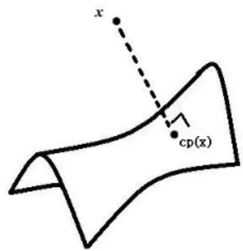
For any x in space, let cp(x) denote the closest point to x in the surface Σ, that means

|x − cp(x)| = inf

y∈Σ|x − y|. Figure 1 shows an example about relation of x and cp(x). Here we

note that cp(x) is well-defined if x is in a sufficiently small neighborhood of a smooth surface.

Now, we define an embedding PDE on Ω which is the neighborhood of the surface by closest point and replace surface operators by standard Cartesian operators, as

∂F

∂t(x) = G(cp(x), F (cp(x)),∇F (cp(x)), △F (cp(x))) ∀x ∈ Ω. (4)

Since the vector x− cp(x) is normal to the surface Σ, the function F (cp(x)) is a constant normal extension from the surface. If x∈ Σ, the first property implies that

∇F (cp(x)) = ∇sF (cp(x)) =∇sF (x)).

Moreover,∇F (cp(x)) is always tangent to the level-sets of the distance function, so applying the second property at the surface, we obtain

∇ · (∇F (cp(x))) = ∇s· (∇F (cp(x)) = ∇s· (∇sF (x)).

According to the two properties, the embedding PDE (4) is equal to the surface PDE (3) on the surface. It means that, if F is a solution of embedding PDE , then the solution on the surface also satisfies surface PDE. Based on this, the closest point method proceeds by the following two steps:

1. Extend the solution off the surface to each grid node on the computational domain around the surface.

−1.5 −1 −0.5 0 0.5 1 1.5 −1.5 −1 −0.5 0 0.5 1 1.5

Figure 2: The function F which we solved from embedding PDE is defined on ’·’ around of surface, and we use F to approximate surface function f , which is solution for surface PDE.

2. Compute the solution of the embedding PDE using standard finite differences scheme on a Cartesian mesh of the computation domain.

At every time step, the solution of the surface PDE is approximated by the solution of the embedding PDE at the grid points on the computation domain. For example, we use the forward Euler method to solve the heat equation on the surface

fn+1 = fn+ ∆t· △sfn.

We do not treat this surface equation directly. Instead, we assume Fn_{(x) = f}n_{(cp(x)) and}

evolve the equation

Fn+1 = Fn+ ∆t· △Fn

on the regular grid points around of surface, and use Fn+1 _{to approximate the solution f}n+1

4

Level set representation

Following [6,7], we represent a moving surface Σ(t) in Rd _{by zero level set of the signed}

distance function ϕ(x, t) . That is

Σ(t) = {x : ϕ(x, t) = 0} (5) where ϕ(x, t) defined by ϕ(x, t) =      −d(x, t) if x ∈ Σ(t)− 0 if x∈ Σ(t) d(x, t) if x∈ Σ(t)+ where d(x, t) = inf

y∈Σ(t) |x − y| is the distance function , Σ(t)

− _{and Σ(t)}+ _{represent inside and}

outside of the surface, respectively. For example, consider a circle surface, the signed distance function of the circle is ϕ =√x2_{+ y}2− 1.

However, it is difficult to give an explicit formula for the signed distance function of any surface. As in [6], we reinitialize the level set function ϕ0 to the signed distance function ϕ

by evolving the reinitialization equation {

ϕτ + S(ϕ0)(|∇ϕ| − 1) = 0 ϕ(x, 0) = ϕ0

(6)

where τ is pseudo time and S(x) is the signed function taken as 1 in Σ(t)+_, −1 in Σ(t)−

and 0 on the surface. By evolving this equation, the function ϕ will be identically equal to zero on Σ, and |∇ϕ| will converge to 1 on the narrowband of the surface. That means the level set function ϕ(t) will converge to the signed distance function. Figure 3 shows the level set function of an ellipse transformed to the signed distance function after reinitialization precess.

By taking the time derivative of ϕ(x, t) = 0, then we have the Hamilton-Jacobi equation

Dϕ

Dt = ϕt+ u· ∇ϕ = 0 (7)

where u is the surface velocity. Since the surface is represented by the zero level set of ϕ(x, t), we can move the surface by solving the equation (7) for a given initial condition ϕ(x, 0).

Figure 3: The left figure is the level set of the function ϕ0 = x 2 (1.2)2 +

y2

(0.8)2 − 1 to represent an

ellipse. The right figure is level set of ϕ which is reinitialized of ϕ0

5

Numerical method

Based on the closest point method [4,1], we use an implicit scheme to solve the embedding PDE and interpolate the value on the surface by degree-p Lagrange interpolation polynomials. Given the surface function fn_{, the signed distance function ϕ}n_{and the vector field u, we evolve} fn+1 and ϕn+1 by the following steps:

Step1: Evolve the surface Σ(tn+1) which represented by zero level set of ϕn+10 in velocity field u. We solve the Hamilton-Jacobi equation (7) for one time step to move our

sur-face. For spatial discretization, we use the third-order upwind weighted essentially non-oscillatory(WENO) scheme [7] to discretize u· ∇ϕn_{. At each grid point (x}

i, yj)

(u· ∇ϕ)ij = u+Dx−ϕij + u−Dx+ϕij + v+D−yϕij + v−D+yϕij

where x+ = max(x, 0) , x− = min(x, 0) and D_x±ϕij, Dy±ϕij are the one-sided divided

differences for the WENO scheme. In third-order WENO scheme [2], the approximation to ∂ϕ_∂x on left-biased stencil {xi−2, xi−1, xi, xi+1} is

D−_xϕi = 1 2∆x [ (∆+ϕi−1+ ∆+ϕi)− ω−(∆+ϕi−2− 2∆+ϕi−1+ ∆+ϕi−1) ] where ω₋ = 1 1 + 2r2 with r = ε + (∆+_∆−_ϕ i−1)2 ε + (∆+_∆−_ϕ i)2 .

where the notation ∆+ϕi = ϕi+1− ϕi, ∆−ϕi = ϕi − ϕi−1 are forward and backward

difference operators respectively. By symmetry, the approximation to ∂ϕ_∂x on right-biased stencil {xi−1, xi, xi+1, xi+2} is

D+_xϕi = 1 2∆x [ (∆+ϕi−1+ ∆+ϕi)− ω+(∆+ϕi+1− 2∆+ϕi+ ∆+ϕi−1) ] where ω+ = 1 1 + 2r2 with r = ε + (∆+_∆−_ϕ i+1)2 ε + (∆+_∆−_ϕ i)2 .

For time discretization, we use the third-order total variation diminishing(TVD) Runge-Kutta scheme in [11]. Consider the time dependent PDE

dϕ

dt = H(ϕ),

We solve the level set function ϕ0 at the (n+1)th step by

     ϕ1 = ϕn+ ∆tH(ϕn) ϕ2 = 3₄ϕn+₄1ϕ1+∆t₄ H(ϕ1) ϕn+1₀ = 1₃ϕn+ 2₃ϕ2+ 2∆t₃ H(ϕ2)

Step2: We reinitialize the level set function ϕn+1₀ to the signed distance function ϕn+1 _by

evolving the reinitialization equation (6) with initial condition ϕn+1₀ . For time dis-cretization, we also use the third-order total variation diminishing(TVD) Runge-Kutta scheme. For spatial discretization, following in [7] ,we use the spatial discretization for

S(ϕ0)(|∇ϕ| − 1) like WENO scheme

S(ϕ0)(|∇ϕ| − 1)ij = s+ij(

√

(a+₎2_{+ (b}−₎2 _{+ (c}+₎2_{+ (d}−₎2− 1)

+ s−_ij(√(a−)2_{+ (b}+₎2 _{+ (c}−₎2_{+ (d}+₎2− 1)

where sij is numerical approximation to signed function of ϕn+10 given by sij = ϕ0 √ ϕ2 0+ ∆x 2

and notation a, b, c, d are one-sided divided differences for the WENO scheme as

Step3: In this step, we need to find the closest point cp(x), the computational domain Ω1

and Ω2 at time step tn+1. Since ϕ is the signed distance function, ∇ϕ will be the unit

normal vector n at surface for each point at surface. So given any point x around of the surface, the closest point cp(x) of x can be written as

cp(x) = x− ϕ(x)∇ϕ(cp(x)).

Assume that the surface is sufficiently smooth and x is close to the surface, then we

have ∇ϕ(x) = ∇ϕ(cp(x)). So that, we can approximate the closest point cp(x) of x by

cp(x) = x− ϕ(x)∇ϕ(x).

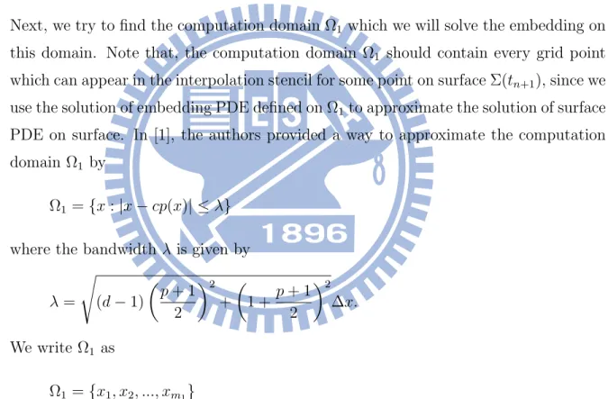
Next, we try to find the computation domain Ω1 which we will solve the embedding on

this domain. Note that, the computation domain Ω1 should contain every grid point

which can appear in the interpolation stencil for some point on surface Σ(tn+1), since we

use the solution of embedding PDE defined on Ω1 to approximate the solution of surface

PDE on surface. In [1], the authors provided a way to approximate the computation domain Ω1 by

Ω1 ={x : |x − cp(x)| ≤ λ}

where the bandwidth λ is given by

λ = √ (d− 1) ( p + 1 2 )2 + ( 1 + p + 1 2 )2 ∆x. We write Ω1 as Ω1 ={x1, x2, ..., xm1}

Let Ω2 be disjoint from Ω1 which contains every grid point which will be used in the

finite difference scheme as

Ω2 ={xm1+1, xm1+2, ..., xm1+m2}

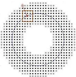
Figure 4 shows an example of the two set Ω1 and Ω2 on a circle with the usage of

Figure 4: Example of unit circle with degree-4 Lagrange interpolation polynomials. The grid points in Ω1 denote•, and grid point in Ω2 are denote ◦. Grid points × are closest point of ⋄, and the grid points in the square are interpolation stencil of ×

Step4: In this step, we use implicit closest point method to solve our problem. Consider the embedding PDE which is defined on Ω1 for our convection-diffusion equation as

Ft(x) + u· ∇F (cp(x)) + (∇s· u)F (cp(x)) =

1

P es△F (cp(x))

(8) Let we denote the vectors

F = [F (x1), F (x2), ..., F (xm1)]

F∗₁ = [F (cp(x1)), F (cp(x2)), ..., F (cp(xm1))]

F∗₂ = [F (cp(xm1+1)), F (cp(xm1+2)), ..., F (cp(xm1+m2))]

We discretize the differential operators of (8) by central difference. Since ∇s · u = ∇ · u − (∇ϕ)t· ∇u · ∇ϕ. , we can write formula (8) into a matrix form

∂ ∂tF = K ( F∗₁ F∗₂ ) (9) where K is m1 by m1+ m2 matrix.

From the closest point method, we let Fn be the normal extension from fn of the surface Σ(t ), that is Fn_{(x) = f}n_{(cp(x)). By using the Crank-Nicolson scheme, we}

have Im1F n+1₋ ∆t 2 K ( F∗₁n+1 F∗₂n+1 ) = Im1F n +∆t 2 K ( F∗₁n F∗₂n ) = b (10)

where Im1 is an m1 by m1identity matrix. Note that, we approximate the value of f n+1

at any point in the surface by Fn+1. Since cp(xi) is at the surface, we apply degree-p

Lagrange interpolation polynomials and then obtain for any index 1 ≤ i ≤ m1+ m2

Fn+1(cp(xi)) = fn+1(cp(xi)) = (p+1)d ∑ s=1 lisF n+1_(x is)

where xis in Ω1 and lis is the Lagrange coefficient for F

n+1_(x is). Rewrite it in a matrix form ( F∗₁n+1 F∗₂n+1 ) = EFn+1 (11)

where E is a m1+ m2 by m1 extension matrix with the entries

eij =     

lis if xj is in the interpolation stencil for cp(xi)

( i.e. j = is for some 1≤ s ≤ (p + 1)d )

0 otherwise

We let M = KE, and combine the two formulae (10),(11), we have

AFn+1 = b (12) where A = Im1 − ∆t 2 M, is an m1 by m1 matrix.

Step5: Once we solve Fn+1_{, then we can approximate the value of f}n+1 _{at surface. By}

exam-ining the spectra of M given in Figure.5(left), the matrix M has some eigenvalues with positive real parts. From (9)(11), we have

∂

these positive eigenvalues will cause the solution an exponential growth and lead to instability. For example, Figure.6(left) shows the oscillatory results for heat equation on a circle using the implicit closest point method with M . Theoretically, it should not occur in our solution, because we have the diffusion term in our equation. So that, we should stabilize the matrix M . Let

f

M = D + (K − D)E

where D is diagonal matrix of K. That means the stabilized form of our system is

∂

∂tF (xij) =−

1

2∆xu· (F (cp(xi+1,j))− F (cp(xi−1,j)), F (cp(xi,j+1))− F (cp(xi,j−1)))

− (∇s· u) F (xi,j) (13)

+ 1

P es(∆x)2

(F (cp(xi+1,j)) + F (cp(xi−1,j)) + F (cp(xi,j+1)) + F (cp(xi,j−1)) −4F (xi,j))

where the only change is that the diagonal entries. This modification will increase the value of diagonal of the matrix. Note that, the system (13) also matches the surface PDE at the surface, because cp(x) = x for any x on the surface. So we can solve Fn+1

by the system (13) and use Fn+1 _{to interpolate the f}n+1 _{at the surface Σ(t} n+1).

−30 −25 −20 −15 −10 −5 0 5 −1.5 −1 −0.5 0 0.5 1 1.5 −30 −25 −20 −15 −10 −5 0 5 −1.5 −1 −0.5 0 0.5 1 1.5

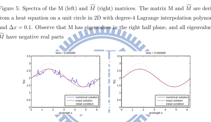
Figure 5: Spectra of the M (left) and fM (right) matrices. The matrix M and fM are derived

from a heat equation on a unit circle in 2D with degree-4 Lagrange interpolation polynomial and ∆x = 0.1. Observe that M has eigenvalues in the right half plane, and all eigenvalues of f

M have negative real parts

0 1 2 3 4 5 6 0 0.5 1 1.5 2 2.5 3 3.5 time = 0.500000 arclength s f(s) numerical solution exact solution initial condition 0 1 2 3 4 5 6 0 0.5 1 1.5 2 2.5 3 3.5 time = 0.500000 arclength s f(s) numerical solution exact solution initial condition

Figure 6: Stable and unstable solutions of the heat equation on a unit circle embedded in 2D with ∆x = 0.1 and degree-4 interpolation

6

Numerical results

In this section, the Peclet number P es is set to be 1, except that in the last example.

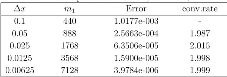
Example 1.

Consider the heat equation on a unit circle

ft=△sf

with the initial condition f0(x, y) = sin θ + 2 defined on surface where θ = sin−1(√ y x2_+y2).

We know the surface Laplacian operator on the circle in polar coordinate is

△sf =

1

r2 ∂2f ∂θ2,

which implies that the function f (x, y, t) = e−tsin θ + 2 is the exact solution of heat equa-tion with initial condiequa-tion f0. We apply the implicit closest point method to the problem

with degree-4 Lagrange interpolation polynomials, and the closest point of (x, y) is given by

(x,y) √

x2_+y2. We use the time step-size ∆t = ∆x = ∆y and compute up to final time T = 1. In

Table 1, the errors at the final time T are computed on Σ with infinity-norm. The results give the rate of convergence about second-order.

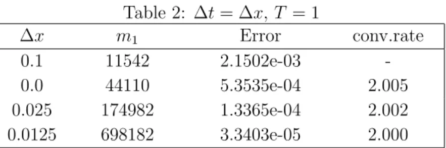
Example 2.

Consider an example in 3D. The heat equation on a unit sphere

ft=△sf

Table 1: Heat equation on a circle, ∆t = ∆x, T = 1

∆x m1 Error conv.rate 0.1 440 1.0177e-003 -0.05 888 2.5663e-004 1.987 0.025 1768 6.3506e-005 2.015 0.0125 3568 1.5900e-005 1.998 0.00625 7128 3.9784e-006 1.999

Table 2: ∆t = ∆x, T = 1 ∆x m1 Error conv.rate 0.1 11542 2.1502e-03 -0.0 44110 5.3535e-04 2.005 0.025 174982 1.3365e-04 2.002 0.0125 698182 3.3403e-05 2.000

with initial condition f0(x, y, z) = xy defined on surface. The surface Laplacian operator on

sphere in spherical coordinate system is

△sf = 1 r2_{sin θ} ∂ ∂θ(sin θ ∂f ∂θ) + 1 r2_sin2_θ ∂2f ∂ϕ2

with x = r sin θ cos ϕ, y = r sin θ sin ϕ and z = r cos θ. Then the function f (x, y, z) = e−6txy

is an exact solution of diffusion equation with initial condition f0 on a unit sphere. The

closest point of (x, y, z) is given by √(x,y,z)

x2_+y2_+z2 in our method, and we compute up to final

time T = 0.5 with time step-size ∆t = ∆x = ∆y = ∆z. The result is shown in Table 2. We can observe that the rate of convergence is also second-order.

Example 3.

Following the Example 1, we also use the same initial function f0(x, y) = sin θ + 2 on a unit

circle Σ where θ = sin−1(√ y

x2_+y2), and we give the velocity field

u = √(−y, x) x2_{+ y}2.

In the Figure 7, the velocity field u is always tangent to the surface Σ at any point in surface. The surface will rotate counterclockwisely but not change the shape itself. That means the level set function which we use to represent the unit circle does not change, so we do not need to solve the Hamilton-Jacobi equation (6) and (7) in our numerical process. We consider the convection-diffusion equation on Σ as

ft+ u· ∇sf =△sf.

If we use the polar coordinates, the equation on the surface Σ can be rewritten as

ft+ ∂f

∂θ =

∂2f ∂θ2.

−1.5 −1 −0.5 0 0.5 1 1.5 −1.5 −1 −0.5 0 0.5 1 1.5

Figure 7: The black curve is unit circle and the green arrow is velocity field. The velocity is given such that the surface rotates counterclockwisely

Table 3: convection diffusion equation on a unit circle, ∆t = ∆x, T = 1

∆x m1 Error conv.rate 0.1 440 5.2753e-004 -0.05 888 1.3152e-004 2.004 0.025 1768 3.2961e-005 1.996 0.0125 3568 8.2431e-006 2.000 0.00625 7128 2.0611e-006 2.000

Then the function f (x, y, t) = e−tsin (θ− t) + 2 is an exact solution of convection-diffusion equation with initial condition f0. We use the time step-size ∆t = ∆x = ∆y and the

numerical results at final time T = 1 are reported in Table 3.

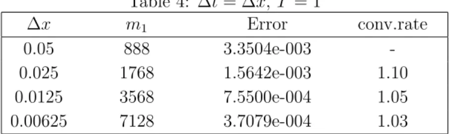
Example 4.

In this example, we give a simple velocity field u = (1, 0). The surface in the velocity field will move along x-axis with unit speed. We solve the convection-diffusion equation with the same initial function f0 and initial surface as in Example 1. The function defined on surface

f (x, y, t) = e−tsin(θ) + 2, where θ(t) = sin−1(√ y

(x−t)2_+y2) is an exact solution of

ft+ u· ∇sf =△sf

with initial condition. In Table 4, we show the result with using signed distance function ϕ to represent the surface Σ(t) and exactly closest point at each time.

Figure 8: The moving surface and surfactant concentration at different time

Example 5.

In this example, we consider the problem      ft+ u· ∇sf + (∇s· u)f = △sf on Σ(t) f (x, y, 0) = f0(x, y) on Σ(0) dx dt = u x∈ Σ(t)

Let velocity field

u = (0, x

2)

be a shear flow, the surface in the flow will move and deform. The initial surface is given by the zero level set of ϕ(x, y, 0) =√(x2_{+ y}2_{)−1 which is a unit circle and the initial surfactant}

concentration on the surface is f0(x, y) = sin(θ) + 2 = y + 2.

Table 4: ∆t = ∆x, T = 1 ∆x m1 Error conv.rate 0.05 888 3.3504e-003 -0.025 1768 1.5642e-003 1.10 0.0125 3568 7.5500e-004 1.05 0.00625 7128 3.7079e-004 1.03

Consider the domain of level set function to be [−1.5, 1.5]×[−2, 2]. Compute the problem up to final time T = 1 with time step-size ∆t = ∆x and take about 10 time steps to reinitialize the level set in our numerical process in each time step. The errors and rates of convergence are shown in Table 5. In this example, the total mass of surfactant on the surface is conserved, and the volume (area) of the interior region enclosed by the moving surface is also conserved since we use a divergence free velocity field. In [6], the total mass of surfactant f on the surface can be written as

M =

∫

Rn

f (x)δ(ϕ(x))|∇ϕ(x)| dx,

and the volume (area) of the interior region is

V =

∫

Rn

1− H(ϕ(x)) dx.

where H is Heaviside function and δ(ϕ) = H′(ϕ). We approximate the Heaviside function H and delta function δ by

H(ϕ) =      0 if ϕ <−ε 1 2 + ϕ ε + 1 2πsin πϕ ε if − ε ≤ ϕ ≤ ε 1 if ε≤ ϕ δ(ϕ) =      0 if ϕ <−ε 1 2ε + 1 2εcos πϕ ε if − ε ≤ ϕ ≤ ε 0 if ε≤ ϕ

with ε = 1.5∆x. Figure 9 shows the relative errors for total mass of surfactant on the surface and the area enclosed by the surface, respectively. The relative error for total mass of surfactant is about 10−3, and the relative error of the area is near 10−6. The moving surface and surfactant concentration on the surface at different times are shown in Figure 10.

Example 6.

In this example, we change the velocity field in Example 5 to

u =

{

(y2_{, 0) if y ≥ 0}

(−y2, 0) if y < 0

which is like a shear flow, and the initial condition for surfactant concentration and surface

Table 5: Error = ∥ f − fref ∥∞, ∆t = ∆x, T = 1 ∆x m1 Error conv.rate 0.05 924 6.4168e-003 -0.025 1850 3.0279e-003 1.08 0.0125 3714 1.3117e-003 1.21 0.00625 7436 4.3986e-004 1.58 0.003125 14844 -

-Figure 9: Relative error for total mass (left) and area (right) at each time

0 0.2 0.4 0.6 0.8 1 0 0.2 0.4 0.6 0.8 1 1.2x 10 −3 t Mass(t) 0.25 0.125 0.0625 0.03125 0 0.2 0.4 0.6 0.8 1 0 0.5 1 1.5 2 2.5 3 3.5 4x 10 −6 t Area(t) 0.25 0.125 0.0625 0.03125

We computed the solution up to final time T = 1 with time step-size ∆t = ∆x = ∆y and take about 20 time steps to reinitialize the level set in our numerical process in each time step. In order to make sure the stability of solving the Hamilton-Jacobi equation (6), we choose the time step-size ∆t = ∆x

4 . The result is shown in Table 6 Figures 11 shows the relative errors

for total mass of surfactant on the surface and the area enclosed by the surface, respectively. The error for total mass of surfactant is still around 10−3, and that of the area enclosed by surface is in the order of 10−6. The moving surface and surfactant concentration on the surface at different time are shown in Figure 12.

Table 6: Error = ∥ f − fref ∥∞, ∆t = ∆x₄ , T = 1

∆x m1 Error conv.rate

0.0125 4056 3.9977e-003

-0.00625 8122 1.2875e-003 1.63

-Figure 10: The moving surface and surfactant concentration at different time

Figure 11: Relative error for total mass (left) and area (right) at each time

0 0.2 0.4 0.6 0.8 1 0 0.2 0.4 0.6 0.8 1 1.2 1.4 1.6 1.8x 10 −3 t Mass(t) 0.125 0.0625 0.03125 0 0.2 0.4 0.6 0.8 1 0 1 2 3 4 5 6 7 8 9x 10 −6 t Area(t) 0.125 0.0625 0.03125

Example 7.

In this example, we construct a surface PDE which has an exact solution with given initial condition. Let f (x, y, t) = e−txy + 2 and the velocity field u = (0,x₂), and we add a source term g to the convection diffusion equation which is given by

g = ft+ u· ∇sf + (∇s· u)f − △sf

Table 7: ∆t = ∆x, T = 1 ∆x m1 Error conv.rate 0.05 924 3.6077e-003 -0.025 1850 1.7042e-003 1.08 0.0125 3712 8.3113e-004 1.04 0.00625 7436 4.1031e-004 1.02

Consider the problem      ft+ u· ∇sf + (∇s· u)f = △sf + g on Σ(t) f (x, y, 0) = f0(x, y) on Σ(0) dx dt = u x∈ Σ(t)

then f is an exact solution of the problem with initial condition f0(x, y) = f (x, y, 0). In our

numerical process, the embedding PDE of the problem is

ft(x) + u· ∇f(cp(x)) + (∇s· u)f(cp(x)) = △f(cp(x)) + g(cp(x))

where g is compute by

g =ft+ u· (∇f − (∇f · n)n) + (∇s· u)f − (△f − n · ∇(∇f) · n)

and approximate n by ∇ϕ where ϕ is signed distance function of the surface Σ(t). The computational domain for level set function is a rectangle [−2, 2] × [−1.5, 1.5]. Compute the solution up to final time T = 1 with time step-size ∆t = ∆x = ∆y, and take about 10 time steps to reinitialize the level set in our numerical process in every time step. The numerical result at final time T is shown in Table 7.

Example 8.

Consider a 3D example. Give a function f (x, y, z) = xyz defined on a unit sphere and the velocity field u = (1, 0, 0) such that the surface in the flow will move along x-axis with unit speed. Similar to previous example, we add a source term g to the convection diffusion equation to make the problem

     ft+ u· ∇sf =△sf + g on Σ(t) f (x, y, 0) = f0(x, y) on Σ(0) dx dt = u x∈ Σ(t)

Table 8: ∆t = ∆x, T = 1

∆x m1 Error conv.rate

0.1 11542 9.9516e-03

-0.05 44110 4.8172e-03 1.046 0.025 174982 2.3653e-03 1.026

having an exact solution with initial condition f0 = f (x, y, z, 0) = xyz. Since we know the

position of surface at any time step, we do not need to solve the equation about the level set function. The closest point of (x, y, z) is given by √ (x−t,y,z)

(x−t)2_+y2_+z2 + (t, 0, 0) at any time

step in our process . We compute the solution up to final time T = 1 with time step-size ∆t = ∆x = ∆y = ∆z, and the numerical result at final time is shown in Table 8.

Example 9.

In this example, we are interested in the effect of surfactant concentration on the surface under the fixed velocity field but with different Peclet numbers. We set the initial condition

f0(x, y, z) = 1, which is constant function defined on the unit sphere, and the velocity field

u = (y₂, 0, 0). Consider the problem

     ft+ u· ∇sf + (∇s· u)f = _{P e}1_s△sf on Σ(t) f (x, y, z, 0) = f0(x, y, z) on Σ(0) dx dt = u x∈ Σ(t)

We use different values of Peclet number in our numerical test. The result of surfactant concentration on the surface at different times are shown in Figure 13,14 and 15, and Figure 16 shows the relative error for total mass of surfactant on the surface. We can observe that the flow will move surfactant to the tip points of the surface, and the surfactant concentration is decreasing since the surface area is increasing.

Figure 13: Peclet number = 2

Figure 14: Peclet number = 1

Figure 15: Peclet number = 0.5

7

Conclusion

In this paper, we apply an implicit closest point method to solve convection-diffusion equation on the moving surface, and use level set function to capture the moving surface. In closest point method, the way to find the closest point is important. Since we represent the surface by signed distance function, we can easily find the closest point in our numerical method. In the numerical test, our algorithm demonstrates good results for the rate of convergence and error of total mass.

Appendix

We prove the fundamental property 2. Assume that the velocity field u is tangent to the level-sets of the distance function, i.e., u· n = 0. By the definition of surface divergence operator, we just need to show that nt· ∇u · n = 0. Take gradient on both sides of u · n = 0,

we have 0 =∇u · n =∇(u1n1+ u2n2) = [ ∂ ∂x(u1n1+ u2n2) ∂ ∂y(u1n1+ u2n2) ] = [ ∂ ∂x(u1)n1 + ∂ ∂x(u2)n2 ∂ ∂y(u1)n1+ ∂ ∂y(u2)n2 ] + [ u1_∂x∂(n1) + u2_∂x∂(n2) u1_∂y∂(n1) + u2_∂y∂ (n2) ] = [ n1 n2 ] [ ∂ ∂x(u1) ∂ ∂y(u1) ∂ ∂x(u2) ∂ ∂y(u2) ] + [ u1 u2 ] [ ∂ ∂x(n1) ∂ ∂y(n1) ∂ ∂x(n2) ∂ ∂y(n2) ] = nt∇u + ut∇n Then (nt· ∇u) · n = −(ut· ∇n) · n =−ut [ ∇n1· n ∇n2· n ] = 0

because n1 and n2 only vary along tangent direction. Then we have ∇su =∇u − nt· ∇u · n

References

[1] Steven J. Ruuth, Barry Merriman, A simple embedding method for solving partial dif-ferential equations on surfaces, Journal of Computational Physics 227(3)(2008) p.1943-1961.

[2] Guang-Shan Jiang, Danping Peng, Weighted ENO schemes for Hamilton-Jacobi equa-tions, SIAM Journal on Scientific Computing 21(6) p.2126-2143.

[3] Chohong Min, On reinitializing level set functions, Journal of Computational Physics 229(8)(2010) p.2764-2772.

[4] Colin B. Macdonald, Steven J. Ruuth, The implicit closest point mwthod for the nu-merical solution of partial differential equation on surfaces, SIAM Journal on Scientific Computing 31(6)(2009) p.4330-4350.

[5] G. Dziuk, C. M. Elliott, Finite elements on evolving surfaces, IMA Journal of Numerical Analysis 27(2)(2007) p.262-292.

[6] Stanley Osher, Ronald Fedkiw, Level set methods and dynamic implicit surfaces, Spring(2003).

[7] Jian-Jun Xu, Hong-Kai Zhao, An eulerain formulation for solving partail differenctial equation along a moving interface, Journal of Scientific Computing 19(1-3)(2003) p.573-594.

[8] H. Wong, D. Rumschitzki, and C. Maldarelli, On the surfactant mass balance at a deforming fluid interface, Physics of Fluid 8(11)(1996) p.3203-3204.

[9] H. A. Stone, A simple derivation of the time-dependent convective-diffusion equation for surfactant transport along a deforming interface, Physics of Fluids 2(1)(1990) p.111-112. [10] Huaxiong Huang, Ming-Chih Lai, Hsiao-Chieh Tseng, A parametric derivation of the surfactant transport equation along a deforming fluid interface, Frontiers of Applied and Computational Mathematics, ed. by D. Blackmore et al.(2008) p.198-205.

[11] Chi-Wang. Shu, Total-variation-diminishing time discretization, SIAM Journal on Sci-entific and Statistical Computing 9(6)(1988) p.1073-1084.

[12] Ming-Chih Lai, Yu-Hau Tseng, Huaxiong Huang, An immersed boundary method for interfacial flows with insoluble surfactant, Journal of Computational Physics 227(2008) p.7279-7293.

[13] Ashley J. James, John Lowengrub, A surfactant-conserving volume-of-fluid method for interfacial flows with insoluble surfactant, Journal of Computational Physics 201(2004) p.685-722.

[14] Xiaofeng Yang, Ashley J. James, An arbitrary Lagrangian-Eulerian (ALE) method for interfacial flows with insoluble surfactants, Fluid Dynamics and Materials Processing 3(1)(2007) p65-96.